CHAPTER 20

WHEN TOPOLOGY CONTROLS GEOMETRY

And now remains,
That we find out the cause of this effect,
Or rather say the cause of this defect,
For this effect defective comes by cause.
Thus it remains and the remainder thus.
—William Shakespeare, Hamlet¹

For most of this book we have been moving away from the rigid confines of geometry, working instead in the much more fluid environment of topology. In this chapter and the next we return to geometry. We will examine polygons, polyhedra, curves, and surfaces, made not of rubber, but of the hardest steel. However, these geometric objects can still be viewed with a topological eye—the polygons and curves are homeomorphic to a circle, and the polyhedra and surfaces are homeomorphic to a sphere or a g-holed torus.

We will present a collection of theorems that shows the surprising relationship between the topology of these shapes and their geometry. We will see how the Euler number can predict certain geometric properties. Our ultimate goal is to present three theorems. In this chapter we will see Descartes’ formula for polyhedra and the angle excess theorem for surfaces, and in the next chapter we will investigate the Gauss-Bonnet theorem for surfaces. These show that certain global geometric properties (related to angles and curvature) are completely determined by topology (given by the Euler number). In this way we will see how topology can control geometry.

Before looking at these theorems for polyhedra and surfaces, we will investigate the analogous results in dimension one. The 1-dimensional analogues of a polyhedron and a surface are a polygon and a simple closed curve, respectively. The first theorem is encountered in any elementary geometry class (see figure 20.1).

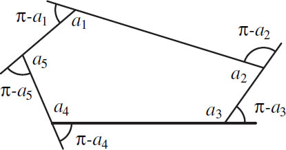
Figure 20.1. The exterior angles of a polygon.

Figure 20.2. The exterior angles of a polygon sum to 2π.

George Pólya (1887–1985) discovered the following short and elegant proof of the exterior angle theorem for convex polygons.² At each corner, draw two line segments pointing outward, one line segment perpendicular to each side (see figure 20.2). Draw a sector of a unit circle at each vertex with these segments as sides. Observe that the angle made by these two segments is precisely the exterior angle. This is true because the two right angles add up to π, so the interior angle and the angle of the sector must also add up to π. Because the sides of each pair of adjacent sectors are parallel, we can reassemble the sectors to form a circle. So, the sum of the exterior angles is 2π. We omit the proof for nonconvex polygons, but it follows from the observation that any nonconvex polygon can be decomposed into convex ones.

In a sense, the exterior angle theorem is not surprising. A car driving along a polygonal road would have to turn at each corner, and the size of each turn is the exterior angle. In order to return to the starting position, the car would have to turn through a total angle of 360°.

Although the typical adult may be hard pressed to remember the quadratic formula or the Pythagorean theorem, there is one mathematical result that almost any adult can quote: the sum of the interior angles of a triangle is 180° (or as we say, π radians). The 180° theorem is a simple consequence of the exterior angle theorem. If a, b, and c are the interior angles of a triangle, then π − a, π − b, and π − c are the exterior angles. By the exterior angle theorem (π − a) + (π − b) + (π − c) = 2π. Rearranging terms yields a + b + c = π.

For polygons other than triangles, the interior angles sum to more than 180°, but the sum still depends only on the number of sides. If a₁, . . . , a_n are the interior angles of a polygon, then by the exterior angle theorem

2π = (π − a₁) + (π − a₂) + . . . + (π − a_n).

Rearranging terms yields the following useful theorem.

To ease the transition to Descartes’ formula for polyhedra, it will be helpful to look at the exterior angles of a polygon in a slightly different way. Think of the corners of a polygon as being “imperfect” straight lines. Looking at each angle, we ask how much the bend differs from a straight line. At a corner with interior angle a the curve differs from a straight line by π − a, the exterior angle. Taking this point of view, we will call π − a the angle deficit or angle defect of the corner. So we rephrase the exterior angle theorem as follows.

There is a smooth analogue of the exterior angle theorem. Consider, again, the car analogy. A Grand Prix race course is a winding, curvy road that loops back to its starting point. As a Formula One race car navigates the track it swerves right, left, right, and left, but by the time it returns to the starting line it has made one complete circuit counterclockwise. In other words, allowing the left and right turns to cancel, the car winds through a total 360° of left-hand turns.

Figure 20.3. The tangent vectors of simple closed curves turn through 2π.

Now, consider a smooth simple closed curve in the plane (the race course; see figure 20.3). Pick an orientation on the curve, then place tangent vectors on the curve pointing in this direction (the headlights of the car). We are interested in the behavior of these tangent vectors as we proceed once around the curve. If the curve is a circle, then as we go around the circle one time counterclockwise, the vectors turn around one time counterclockwise as well—they turn through an angle of 2π. Here it may be helpful to think of a tangent vector as being the needle of a dial. As we move the dial around the circle, the needle turns around exactly one time counterclockwise. For a more complicated curve, as the dial traverses the curve, the needle may move forward and backward, but in the end it travels exactly once around the dial.

Although this observation may seem obvious (as it was believed to be for a long time), it is difficult to prove. In 1935 Hopf proved the theorem.³ It is known as Hopf’s Umlaufsatz, or more simply, the theorem of turning tangents.

It is not difficult to see the relationship between the exterior angle theorem and the theorem of turning tangents. In fact, it is possible to state a theorem that is a hybrid of these two in which the curve is smooth except for a finite number of sharp corners. A car driving on a curvy road that occasionally has to make sharp turns, turns through 360° by the time it returns to its starting location.

Returning to the original assertion, we ask, how do these theorems bridge two mathematical subjects? They show a sense in which topology can control geometry. A topologist cannot tell the difference between polygons and smooth simple closed curves. They are all circles. A topologist does not talk about angles, straightness, tangent vectors, and so on. To a geometer every polygon and every simple closed curve is different from the rest, and he describes these objects by speaking of their corners, their curvature, and other descriptors. The exterior angle theorem and the theorem of turning tangents say that being homeomorphic to a circle completely determines a geometric property—the total angle deficit of the shape. Regardless of how many bends it has, the total angle deficit is 2π.

Figure 20.4. The corner of a cube has angle deficit π/2.

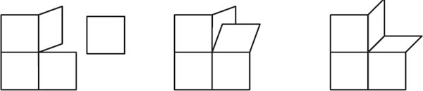
Figure 20.5. This corner has angle excess π/2.

We now investigate how these two theorems generalize to Descartes’ formula for polyhedra and the angle excess theorem for surfaces.

Get a square piece of paper, a pair of scissors, and tape. Divide the paper into four equal quadrants, and use the scissors to cut one of them away (set this piece aside for later). Then tape together the two cut edges to obtain an object that looks like the corner of a rectangular box (see figure 20.4).

We defined the angle deficit at a corner of a polygon to be the amount by which the bend failed to be a straight line. Likewise, define the angle deficit of a solid angle to be the amount by which it fails to be a flat plane. In our example, four right angles (2π) met at the center of our paper, then we cut one away (leaving 3π/2). Thus the angle deficit at the corner of a cube is 2π − 3π/2 = π/2.

Take another square piece of paper. As before, divide it into quadrants. Cut once from the edge to the center (see figure 20.5). Take the discarded piece from the first construction and tape the two cut edges to the cut on the folded paper. Doing so we see that there is too much angle present. We get a configuration that resembles a brick wall with a brick removed. The central vertex has a total angle of 5π/2, and that is π/2 more than a flat plane. We call this an angle deficit of −π/2, or an angle excess of π/2.

Figure 20.6. This nonconvex polyhedron still has total angle deficit 4π.

A polyhedron has many vertices, each with its own angle deficit (or angle excess). The total angle deficit of a polyhedron is the sum of all of its angle deficits.

Consider some examples. Each of the eight corners of a cube has an angle deficit of π/2, so the total angle deficit is 4π. The four faces of a tetrahedron are equilateral triangles. Since three equilateral triangles meet at each vertex, the angle deficit at each corner is 2π − 3(π/3) = π. There are four vertices, so the total angle deficit is 4π. Finally, consider the nonconvex polyhedron in figure 20.6: a large cube with a smaller cube removed from one of its corners (think of a Rubik’s cube with a corner piece pulled out). The corners marked 1–10 have angle deficit π/2. Corner 11 is facing the “wrong way” but it still has angle deficit π/2. The three remaining corners (12, 13, and 14) have angle excesses of π/2. Thus the total angle deficit is 11(π/2) + 3(−π/2) = 4π.

At this point the pattern is becoming clear, and we conjecture that every polyhedron has a total angle deficit of 4π. This observation was first made by Descartes in his unpublished notes that we discussed in chapter 9, The Elements of Solids. The third sentence of Descartes’ notes reads:

As in a plane figure [polygon] all the exterior angles, taken together, equal four right angles [2π], so in a solid body [polyhedron] all the exterior solid angles [angle deficits], taken together, equal eight solid right angles [4π].⁴

Figure 20.7. The total angle deficit of the torus is zero.

As Descartes pointed out, the parallels with the exterior angle theorem are self-evident. Just as the sum of the angle deficits of a polygon is 2π, the sum of the angle deficits of a polyhedron is 4π.

A slight variant of this theorem was rediscovered by Euler and appeared in his papers on the polyhedron formula.⁵ Euler proved that the sum of all plane angles in a polyhedron with V vertices equals 2π (V − 2). Where Descartes’ formula generalizes the exterior angle theorem for polygons, Euler’s formula generalizes the interior angle theorem. It is easy to see that Euler’s result is equivalent to Descartes’. The total angle deficit is simply 2π V minus the sum of all plane angles, or 2π V − 2π (V − 2) = 4π.

Of course, both Euler and Descartes were considering convex polyhedra. It turns out that with a little modification, the theorem applies to all polyhedra, even those that are not topological spheres. The total angle deficit is a topological invariant, and it has a simple relationship with the Euler number of the polyhedron.

The cube, tetrahedron, and broken cube are topological spheres and have Euler number 2, so the total angle deficit is 2π χ(P) = 2π. 2 = 4π. As a nonspherical example, consider the polyhedral torus shown in figure 20.7. It has sixteen corners, eight of which have an angle deficit of π/2 and eight which have an angle excess of π/2 (angle deficit of −π/2). So, the total angle deficit is zero, the Euler number of the torus. The reader is encouraged to verify Descartes’ formula for the paper polyhedra in appendix A.

Figure 20.8. For an n-gon, (a₁ + . . . + a_n) − nπ + 2π = 0.

We now prove Descartes’ formula. Let P be a polyhedron with V vertices, E edges, and F faces, and let T be the total angle deficit of P. We must show that T = 2π χ(P) = 2πV − 2π−E + 2π F.

Choose any face of the polyhedron. Suppose it has plane angles a₁, . . . , a_n. By the interior angle theorem,

a₁ + . . . + a_n = (n−2)π.

Rearranging the terms yields

(a_l + . . . + a_n) − nπ + 2π = 0.

We can visualize this equality as follows. If we put −π on each edge of the face, the angle measure at each corner, and 2π in middle of the face (see figure 20.8), then the sum of these quantities is zero.

Now, do the same for every face of P and add up all of these quantities. Each face contributes 2π and each edge contributes −2π (−π from each side). So,

S − 2π E + 2π F = 0,

where the S is the sum of all plane angles in P. Now add T, the total angle deficit, to each side of the equality,

(T + S) − 2π E + 2π F = T.

Because T is the total angle deficit, then by adding T, we are adding enough so that the angle sum at each vertex can again be 2π. In other words, T + S is 2π V. So, T = 2π V − 2π E + 2π F = 2π χ(P).

Descartes’ formula is a beautiful illustration of the surprising relationship between topology and geometry. Because the total angle deficit is related to the Euler number, we see that the topology of the polyhedron completely determines one aspect of its global geometry.

As an application of this theorem, the reader is encouraged to find a new proof that there are only five Platonic solids.

In most of this book we have assumed that the edges that partition a surface into faces are topological entities. The edges can wiggle crazily and create faces that are wildly misshapen. In this chapter we are investigating the much less wild and crazy field of geometry. Ideally we would like our faces to be polygons with straight edges. On a curved surface it is impossible for the edges to be straight, so instead we require that they be geodesic curves.

In chapter 10 we introduced the concept of a geodesic on a sphere. It was any segment of a great circle. It turns out that we can define a geodesic curve on any rigid surface. It is characterized by minimizing length—the shortest path between two points on a surface is realized by traveling along a geodesic curve. The well known saying, “The shortest distance between two points is a straight line” should be “The shortest distance between two points is a geodesic curve.” For the rest of this chapter we assume that the edges on our surfaces are geodesic curves, making the faces geodesic polygons.

One benefit of working with geodesic polygons is that we can measure the angles at the vertices. The edges are curved, but when we zoom in to one of the angles with a strong microscope (figuratively speaking), the edges appear straight, so it is possible to measure the angles.

Triangles in the plane obey the 180° theorem, but on a typical surface, the 180° theorem need not apply. Recall that Harriot and Girard proved that the sum of the interior angles of a geodesic triangle on a sphere exceeds 180° (chapter 10). There are other surfaces, such as saddle-shaped surfaces, for which the sum of the interior angles of a geodesic triangle will be less than 180° (see figure 20.9).

So we can speak about the angle excess or angle deficit of a geodesic triangle—the amount that the interior angle sum differs from that of a planar triangle. That is, the angle excess of a geodesic triangle with interior angles a, b, and c is (a + b + c) − π. If (a + b + c) − π is negative, the triangle has an angle deficit.

Similarly we can define the angle excess or deficit of an n-sided geodesic polygon. By the interior angle theorem, the sum of the interior angles of a planar n-gon is (n − 2)π. So the angle excess of an n-gon with interior angles a₁, a₂, . . . , a_n is (a₁ + a₂ + . . . + a_n) − (n − 2)π.

Figure 20.9. A triangle with an angle excess (left) and one with an angle deficit (right).

Figure 20.10. An octahedron rolled into a ball.

It is important not to confuse angle excess and deficit for polyhedra and for surfaces. A polyhedron has an angle excess or deficit at its vertices, whereas it is the faces on a surface that have angle excesses or deficits. It is confusing that they have the same names, but as we see in the following discussion, they are intimately related.

Take a lump of modeling clay and make an octahedron. Every face is an equilateral triangle, so the angle deficit at each vertex is 2π − 4(π/3) = 2π/3. Since there are six vertices, the total angle deficit is 6(2π/3) = 4π, as guaranteed by Descartes’ formula. Darken each of the edges using a marker. Then place the polyhedron on a table and roll it until it is spherical (figure 20.10). What were triangular faces in the octahedron are now curved. If we roll this shape carefully, the straight edges turn into geodesic segments and the faces become geodesic triangles.

After rolling the octahedron into a ball, there is no longer an angle deficit at any vertex. Rolling it on the table flattens the corners so the angles sum to 2π. Where did the angle deficit go?

Figure 20.11. Labeling a surface with 2π on each face, −π on each side of each edge, and the angle measures at each vertex.

It is not difficult to see that during this process the interior angles of the triangles changed size. The angles meeting at each vertex, which measured 60° before, are now right angles. The triangles on the clay ball have three right angles, so the sum of the interior angles is 3π/2. The triangular faces have an angle excess. The angle deficits at the vertices of the octahedron get distributed among the faces of the ball to become angle excesses in the triangles. Similarly, for any partition of a surface by geodesic polygons, the vertices no longer have angle deficits or angle excesses, but the faces do.

If a surface is partitioned into vertices, geodesic edges, and faces, then the total angle excess is the sum of the angle excesses of all faces. Just as the total angle deficit of a polyhedron is related to its Euler number (Descartes’ formula), the total angle excess of a surface is related to its Euler number. We have the following analogue of Descartes’ formula for surfaces.

The proof of this theorem should look familiar by now. Let S be a surface partitioned into vertices, geodesic edges, and faces. Decorate the surface by putting 2π in the middle of each face, −π on each side of each edge, and the angle measure at each angle (see figure 20.11). If we sum these quantities on a particular n-sided face with interior angles a₁, a₂, . . . , a_n we obtain the angle excess of the face,

2π − nπ + (a₁ + a₂ + . . . + a_n) = (a₁ + a₂ + . . . + a_n) − (n − 2)π.

Thus, adding all quantities on the surface gives the total angle excess of the surface.

On the other hand, each vertex contributes 2π, each edge contributes −2π, and each face contributes 2π. Summing all values yields 2π V − 2π E + 2π F = 2π χ(S), and we have our result.

Descartes’ formula and the angle excess theorem are two beautiful theorems that show a sense in which topology can control geometry. In the next chapter we see another example. We will see that the total curvature of a surface depends on the surface’s topology, and that it depends in an intimate way on the surface’s Euler number.