![11.4 Complementary control of renewable plants with energy storage plants [144]](https://imgdetail.ebookreading.net/cover/cover/data/EB9780128009888.jpg)
11.3.18 Hydrogen Generation and Storage
A well-known way of splitting water (H2O) is by electrolysis [151]. A container (trough) contains distilled water and two electrodes -- the anode (A) and cathode (C) consisting of either platinum or nickel -- connected to a DC current source. Pure H2O is a poor conductor; the addition of H2SO4 to the water makes the solution conducting. Although the solution of H2O and H2SO4 heats up - due to the losses caused by the current flowing from anode to cathode- at the anode oxygen O2 and at the cathode hydrogen H2 is accumulated. The efficiency of splitting H2O based on electrolysis is about ηelectrolysis = 80%, that is, 20% of the energy is converted to heat within the electrolysis process. The energy density of hydrogen is about 2.28 times that of gasoline (Egasoline = 12.3 kWh/kg-force), that is, EH2 = 28 kWh/kg-force. {Note 1 liter (dm3) of water has a mass m of 1 kg at 4° Celsius, and exerts a (force or) weight of 1 kg-force on a scale}. The additional energy loss due to the production of distilled water can be deduced from the definition of unit 1 kcal: The energy of 1 kcal is required to heat 1 kg-force of H2O by 1 ° C (this is approximately true only because the energy required depends upon the temperature range. It is exactly true heating pure water from 14.5°C to 15.5°C). Note that 1 kcal = 4.186 kWs.
11.3.18.1 Application Example 11.7: Production of Hydrogen Based on Electrolysis and its Application with Respect to Electric Cars with Fuel Cells [1]
a) The energy of a Pout = 5 MW wind-power plant can be used to generate hydrogen during 8 hours of operation per day during 365 days per year. The construction cost of the 5 MW plant and the generation of pure water including the electrolysis equipment is $4000/kW installed power capacity. How much hydrogen energy (expressed in MWh) can be obtained during one year taking into account the above-described losses?
b) Calculate the payback period provided one kg-force of hydrogen (weight) can be sold for $4.00. For your payback period calculation you may neglect interest for borrowing the money for the construction cost.
c) How many “equivalent-gasoline gallons” of hydrogen can be produced during one year?
d) Provided a car owner travels 15,000 miles per year with an average mileage of 40 miles/(gallon “equivalent gasoline”), how many car owners can get the “equivalent gasoline gallons of hydrogen” from the 5 MW plant?
Solution to Application Example 11.7
a) The hydrogen that can be produced within one year is given by the total energy available from the wind turbine Etotal = (5 MW)(8 h/day)(365 days/year) = 14,600 MWh. The efficiency of electrolysis reduces this energy to Euseful = 0.8 Etotal = 11,680 MWh. The energy content of 1 kg-force of hydrogen is EH2 = 28 kWh/(kg-force), thus the amount of hydrogen produced is H2 = Euseful/EH2 = 417,143 (kg-force). The atomic weight of hydrogen (H2) is 2 and that of water (H2O) is 18, therefore the amount of H2O required for the electrolysis is H2O = 417,143/(2/18) = 3.754°106 kg-force. The energy loss Edistillation due to the production of distilled water is obtained from ![]() as Edistillation = (3.754·106 kg-force)(0.10465 kWh/kg-force) = 392.9 MWh. The energy available for the electrolysis is now EH2 = Euseful-Edistillation = 11,680 MWh-392.9 MWh = 11,287 MWh.
as Edistillation = (3.754·106 kg-force)(0.10465 kWh/kg-force) = 392.9 MWh. The energy available for the electrolysis is now EH2 = Euseful-Edistillation = 11,680 MWh-392.9 MWh = 11,287 MWh.
b) The payback period -neglecting interest payments- is based on the earnings per year and the construction cost. For H2 = EH2/(EH2 per kg-force) = (11,287·106 Wh)/(28kWh/kg-force) = 403,107 kg-force per year the earnings are Earnings/year = (403,107 kg-force/year)($4.00/kg-force) = $1,612,428/year. The construction cost is Cconstruction = ($4000)(5,000 kW) = $20,000,000 resulting in a payback period of y = ($20,000,000/$1,612,428) = 12.4 years.
c) With EH2 = 11.287·106 kWh, the specific weight of gasoline of γgasoline = 0.72 kg-force/liter = 2.736 kg-force/gallon, and the energy content of gasoline Egasoline = 12.3 kWh/kg-force the weight of gasoline in kg-force is Weightgasoline = 11.287·106 kWh/(12.3kWh/kg-force) = 917,642 kg-force or the equivalent gallons of gasoline produced per year are Gallonsgasoline = 917,642 kg-force/(2.736 kg-force/gallon) = 335,396 equivalent gallons of gasoline per year.
d) Each car owner uses (15,000 miles/year)/(40 miles/gallon) = 375 gallons/year, that is, [335,396 gallons/year]/{375 gallons/(year/owner} = 895 owners. In other words the 5 MW wind-power plant produces enough hydrogen to meet the needs of 895 car owners.
11.3.19 Fuel Cells
A fuel cell takes fuel (e.g., hydrogen and oxygen) as input and produces electricity as output: it will continue to produce output as long as raw material (e.g., fuel) is supplied. This is the difference between a fuel cell and an ordinary battery, except flow batteries. While both rely on electrochemistry a fuel cell is not consumed as an ordinary battery when it produces electricity: it transforms the chemical energy stored in the fuel into electrical energy [1,152].
11.3.19.1 Application Example 11.8: Calculation of the Efficiency of a Polymer Electrolyte Membrane (PEM) Fuel Cell Used as an Energy Source [1]
A PEM fuel cell has the parameters:
Performance: output power = Prat = 2400 W1), output current = Irat = 92 A1), DC voltage range = Vrat = 25 to 50 V, operating lifetime: Tlife = 1500 h2).
Fuel: composition = C = 99.99% dry gaseous hydrogen, supply pressure = p = 10 to 250 PSIG, consumption = V = 37 SLPM3).
Operating environment: ambient temperature = Tamb = 3°C to 30°C, relative humidity = HR = 0% to 95%, location = indoors and outdoors4).
Physical: length x width x height = 56 x 50 x 33 cm, weight = W = 26 kg-force.
Emissions: liquid water = H2O = 1.74 liters maximum per hour.
1) Beginning of life, sea level, rated temperature range
2) CO destroys the proton exchange membrane
3) At rated power output, SLPM ≡ standard liters per minute (standard flow)
4) Unit must be protected from inclement weather, sand and dust.
a) Calculate the power efficiency of a PEM fuel cell in two different ways.
b) Find the specific power density of this PEM fuel cell expressed in W/kg-force.
c) How does this specific power density compare with that of a lithium-ion battery?
Hints:
1) The nominal energy density of hydrogen is 28 kWh/(kg-force), which is significantly larger than that of gasoline (12.3 kWh/kg-force). This makes hydrogen a desirable fuel for automobiles.
2) The (weight) density of hydrogen is γhydrogen = 0.0899 g-force/liter.
3) The oxygen atom has 8 electrons, 8 protons and 8 neutrons.
Solution to Application Example 11.8
a) Atomic-weight method: Atomic weights of hydrogen (H), oxygen (O), and water (H2O) is 1, 16, and 18, respectively. If 1.74 liters of water are emitted then the weight of hydrogen consumed is weightH2 = (2/18)(1.74 kg-force/h) = 0.19333 kg-force/h and the corresponding hydrogen input energy provided is EH2 = (0.19333 kg-force/h)(28.kWh/kg-force) = 5.41 kWh/h which corresponds to an input power of Pin = 5.4133 kW. The output power is Pout = 2.4 kW resulting in a power efficiency of η = Pout/Pin = 0.443.
Hydrogen-density method: The input power of hydrogen is Pin = (γhydrogen)(standard flow/h)(EH2/kg-force) = (0.0899·10- 3 kg-force/liter)(37·60 liters/h)(28 kWh/kg-force) = 5.59 kWh/h, or Pin = 5.59 kW yielding a power efficiency of η = Pout/Pin = 0.43.
b) The specific power density per unit of weight is power density = Pout/weight = 2400 W/(26 kg-force) = 92.3 W/kg-force. However, some publications cite PEM fuel cell stacks with power densities over 1,500 W/kg-force. The disadvantage of a fuel cell is that braking energy cannot be stored as can be done by a battery.
c) The power density of a lithium-ion battery is 300 W/kg-force.
11.3.19.2 Solutions to Power Quality Problems of Fuel Cells
The production of hydrogen as a fuel for electric/hybrid cars must be improved. It is conceivable that cars will be built with either combustion engines or fuel cells fed by hydrogen, and small batteries to store the available braking energy. There is not much experience with the safety of handling hydrogen on a large scale in refueling stations -- similar to gasoline infrastructure. It might be better to convert hydrogen at the production site to methane, which is less explosive than hydrogen, and then reconvert methane in the automobile back to hydrogen through a chemical plant the so-called reformer.
11.3.20 Molten Salt Storage
Solar power generation [153–157] around the clock is possible where a solar concentrator array, consisting of thousands of mirrors on the ground and a tower supporting at the focal point of the mirrors a salt container, see Figure 11.23. Figure 11.24 illustrates construction details. The great advantage of this approach is that solar heat can be stored in the molten salt. SolarReserve [153] has developed, constructed and sold solar power systems that have output powers from 100MW to 200MW for a single molten salt power tower. For example, their Crescent Dunes project has 110MW output power that can store and generate energy for 10 hours of full-load output power by focusing mirrors onto millions of gallons of molten salt which flows through a heat exchanger (receiver) producing steam and driving a steam turbine, allowing the plant to provide electricity for 24 hours a day.


The solar energy is generated by a massive circular array of, for example, 10,347 heliostats, each measuring at Crescent Dunes 37 feet wide and 34 feet tall. The heliostat field encircles a concrete solar power tower which is 540 feet high with a 100-foot high receiver on top. Molten salt flows through the receiver, but it is not held there. The molten salt is held in the storage tanks, each tank holding 3.6 million gallons (or 70 million pounds-force) of molten salt. When the heliostats focus the sunlight onto the receiver the salt is heated to over 1,000 degrees Fahrenheit. When it is needed such as at night or at peak times, the heat is released by passing the molten salt through a heat exchanger and steam generator that drives a turbine to produce electricity. The cooled salt is then recirculated to the receiver for re-heating.
The salt used is a mixture of sodium and potassium nitrate (the same as that used in fertilizers), which is inexpensive, reliable, and environmentally friendly. It will be mixed on site with no additives. Apart from a few unique components such as the high heat flux hardware in the tower, the system uses existing technologies such as turbines and steam generators. The system was proven over a four-year period in the 1990s at a 10 MW demonstration project near Barstow in California.
Other solar systems also use salt as storage, but they use synthetic oil in the steam generation. Using salt for both means the system is more efficient, since it can produce steam at higher temperatures and can harvest three times as much energy for the same amount of salt, as compared to the oil approach. The system can be air cooled, thus avoiding criticisms about water use, but its height, at 640 feet (with a maintenance crane on top), could spark other (e.g., environmental) criticisms.
11.3.21 Solutions to Power Quality Problems of Molten Salt Storage
The molten salt approach appears to be best suited for long-term energy storage requiring not necessarily cooling water as discussed above. The disadvantages are the great number of heliostats and the tall tower with the heavy salt container. This approach deserves more research effort as it is suitable for desert areas. Unfortunately such a location requires long transmission lines to transmit the generated power to urban areas.
11.4 Complementary control of renewable plants with energy storage plants [144]
Most renewable energy sources such as PV and WP plants generate intermittently electricity. For this reason energy storage is needed to control in a complementary manner the flow of electrical energy from the renewable and storage plants to the consumer, as well as the flow of energy from the renewable plants to the storage plants.
11.4.1 Energy Efficiency and Reliability Increases Based on Distributed Generation of Interconnected Power System and Islanding Operation
Prior to 1940 there were a limited number of interconnected power systems and the servicing of the load was elementary since the systems were primarily radial circuits (Figure 11.25a) and many power systems were operated in islanding mode. In more recent years, the numerous advantages of interconnection of many power systems were recognized within the three US power grids [1] (Western, Eastern and Texan generation systems [ERCOT]), see Figure 11.25b for example. Many loop circuits with many load/generation buses and high levels of power exchange between neighboring companies exist. The latter point relates closely to interconnection advantages.

With no addition of generation capacity, it is possible to increase generation capability, efficiency and reliability through interconnection. For example, in the case of an outage of a generating unit, power may be purchased from a neighboring company. The cost savings realized from lower installed capacity usually far outweigh the cost of the transmission circuits required to access neighboring companies. Steady-state power flow is discussed in Chapter 7. While on the one hand the energy efficiency of an interconnected system is increased by more fully loading existing generation plants, it is on the other hand decreased by transporting energy via transmission lines over longer distances. Thus on average the transmission loss within interconnected systems is about 8%.
11.4.2 Distributed Power Plants
The generation mix (e.g., coal, natural gas, nuclear, hydro plants) of existing power systems will change in the future to mainly natural-gas fired plants, distributed renewable generation facilities [158] and storage plants. In addition a transition from the interconnected system to an islanding mode of operation must be possible [55] to increase reliability. This means that any islanding system must have a frequency leading plant --called “frequency leader”-- in addition to renewable plants and storage plants. Renewable and storage plants cannot be frequency leaders because of their intermittent and limited output powers, respectively.
11.4.3 Review of Current Methods and Issues of Present-Day Frequency and Voltage Control
Present-day frequency/load and voltage control of interconnected systems take place at the transmission level and are based on load sharing and demand-side management. Load sharing relies on drooping characteristics [49], see Figures 4a, b, c of [144] or Figures 11.26 and E11.9.1 where natural gas, coal, nuclear and hydro plants or those with spinning reserves supply the additional load demand. If this additional load cannot be provided by the interconnected plants then demand-side management (e.g., load shedding) will set in and some of the less important loads will be disconnected. This method of frequency/load control (when no spinning reserve is available) cannot be employed if renewable sources operate at peak power exploiting the renewable sources to the fullest in order to displace as much fuel as possible. This approach works well as long as renewable energy represents a small fraction of the generation capacity, i.e. the highly-variable renewable characteristic on the left side of Figure 11.26 is significantly smaller than the plant with spinning reserve characteristic on the right. As renewable penetrations increase at either the distribution or transmission levels, control problems may result. In present-day interconnected systems a frequency variation between fmax = 59 and fmin = 61 Hz, that is Δf =![]() 1.67% is acceptable [159].
1.67% is acceptable [159].

11.4.4 Control or Frequency/Load Control of an Isolated Power Plant with one Generator only
Figure 11.27 illustrates the block diagram of governor, prime mover (steam turbine) and rotating mass & load of a turbo generator set [49].

11.4.4.1 Application Example 11.9: Angular Frequency Change for a Positive (Acceptance) and a Negative (Rejection) Load Change
Angular frequency change Δω per change in generator output power ΔP, that is R = ![]() 0.01 pu, the frequency-dependent load change ΔPL|frequ per angular frequency change Δω, that is
0.01 pu, the frequency-dependent load change ΔPL|frequ per angular frequency change Δω, that is
D =![]() = 0.8 pu, step-load change
= 0.8 pu, step-load change ![]() pu, angular momentum of steam turbine and generator set M = 4.5, base apparent power Sbase = 500 MVA, governor time constant TG = 0.01 s, valve changing time constant TCH = 1.0 s, and load reference set point load(s) = 1.0 pu:
pu, angular momentum of steam turbine and generator set M = 4.5, base apparent power Sbase = 500 MVA, governor time constant TG = 0.01 s, valve changing time constant TCH = 1.0 s, and load reference set point load(s) = 1.0 pu:
a) Derive for Figure 11.27 Δωsteady state by applying the final value theorem. You may assume load reference set point load(s) = 1.0 pu, and ![]() pu. For the nominal frequency f* = 60 Hz calculate the frequency fnew after the load change has taken place.
pu. For the nominal frequency f* = 60 Hz calculate the frequency fnew after the load change has taken place.
b) List the ordinary differential equations and the algebraic equations of the block diagram of Figure 11.27.
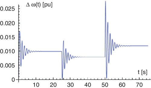
c) Use either Mathematica or Matlab to establish steady-state conditions by imposing a step function for load reference set point load(s) =![]() pu and run the program with a zero-step load change ΔPL = 0 (for 25 s) in order to establish the equilibrium condition without load step. After 25 s impose a step-load change of
pu and run the program with a zero-step load change ΔPL = 0 (for 25 s) in order to establish the equilibrium condition without load step. After 25 s impose a step-load change of ![]() pu to find the transient response of Δω(t) for a total of 50 s and at 50 s impose a step-load change of
pu to find the transient response of Δω(t) for a total of 50 s and at 50 s impose a step-load change of ![]() pu to find the transient response of Δω(t) for a total of 75 s.
pu to find the transient response of Δω(t) for a total of 75 s.
Solution to Application Example 11.9
a) Define the transfer functions ![]() ,
, ![]() ,
, ![]() , and
, and ![]() . From the block diagram one obtains
. From the block diagram one obtains ![]() , where
, where ![]() resulting in
resulting in ![]() . Or
. Or 
At steady state load(s) = 1.0 pu and ![]() pu one obtains with the finite-value theorem the droop characteristic in the frequency-load coordinate system
pu one obtains with the finite-value theorem the droop characteristic in the frequency-load coordinate system  , or for the given parameters
  with frated = f* = 60 Hz one obtains the new frequency fnew = f*- 0.00198°60 Hz = 59.88 Hz.
b) The algebraic and differential equations of the block diagram are:

c) The results based on Mathematica are shown in Figure E11.9.1. The Mathematica input program is listed in Table E11.9.1.
Table E11.9.1
Mathematica input program for isochronous generation
| R = 0.01; d = 0.8; M = 4.5; Tg = 0.01; Tch = 1; Lr = 1; DPL[t_]:=If[t < 50,If[t < 25,0,0.2],-0.2]; ic1 = Dw[0]= = 0; ic2 = DPmech[0]= = 0; | ic3 = DPvalve[0]= = 0; E1[t_]:=Lr-Dw[t]/R; E2[t_]:=DPmech[t]-DPL[t]; eqn1 = Dw'[t]= =(1/M)∗(E2[t]-d∗Dw[t]); eqn2 = DPmech'[t]= =(1/Tch)∗(DPvalve[t]-DPmech[t]); eqn3 = DPvalve'[t]= =(1/Tg)∗(E1[t]-DPvalve[t]); sol = NDSolve[{eqn1,eqn2,eqn3,ic1,ic2,ic3},{Dw[t], DPmech[t], DPvalve[t]},{t,0,75}, MaxSteps- > 100000]; Plot[Dw[t]/.sol,{t,0,75},PlotRange- > All,AxesLabel- > {"t[s]","Dw[t][pu]"}] |
11.4.5 Load/Frequency Control with Droop Characteristics of an Interconnected Power System Broken into Two Areas each Having one Generator
Figure 11.28 shows the block diagram of two generators interconnected by a transmission tie line [49].

11.4.5.1 Application Example 11.10: Instability with Identical Droop Characteristics and Stability with Different Droop Characteristics
Data for generation set (steam turbine and generator) #1: Angular frequency change (Δω1) per change in generator output power (ΔP1), that is R1= ![]() 0.01 pu (e.g., coal-fired plant), the frequency-dependent load change (ΔPL1|frequ) per angular frequency change (Δω1), that is D1=
0.01 pu (e.g., coal-fired plant), the frequency-dependent load change (ΔPL1|frequ) per angular frequency change (Δω1), that is D1= ![]() = 0.8 pu, step-load change
= 0.8 pu, step-load change ![]() pu, angular momentum of steam turbine and generator set M1 = 4.5, base apparent power Sbase = 500 MVA, governor time constant TG1 = 0.01 s, valve charging time constant TCH1 = 0.5 s, and load ref1(s) = 0.8 pu.
pu, angular momentum of steam turbine and generator set M1 = 4.5, base apparent power Sbase = 500 MVA, governor time constant TG1 = 0.01 s, valve charging time constant TCH1 = 0.5 s, and load ref1(s) = 0.8 pu.
Data for generation set (steam turbine and generator) #2: Angular frequency change (Δω2) per change in generator output power (ΔP2), that is R2= ![]() 0.02 pu (e.g., coal-fired plant), the frequency-dependent load change (ΔPL2|frequ) per angular frequency change (Δω2), that is D2=
0.02 pu (e.g., coal-fired plant), the frequency-dependent load change (ΔPL2|frequ) per angular frequency change (Δω2), that is D2= ![]() = 1.0 pu, step-load change
= 1.0 pu, step-load change ![]() pu, angular momentum of steam turbine and generator set M2 = 6, base apparent power Sbase = 500 MVA, governor time constant TG2 = 0.02 s, valve charging-time time constant TCH2 = 0.75 s, and load ref2(s) = 0.8 pu.
pu, angular momentum of steam turbine and generator set M2 = 6, base apparent power Sbase = 500 MVA, governor time constant TG2 = 0.02 s, valve charging-time time constant TCH2 = 0.75 s, and load ref2(s) = 0.8 pu.
Data for tie line: T = ![]() with Xtie = 0.2 pu.
with Xtie = 0.2 pu.
a) List the ordinary differential equations and the algebraic equations of the block diagram of Figure 11.28.
b) Use either Mathematica or Matlab to establish steady-state conditions by imposing a step function for load ref1(s) = ![]() pu, load ref2(s) =
pu, load ref2(s) = ![]() pu and run the program with zero step-load changes ΔPL1 = 0, ΔPL2 = 0 (for 10 s) in order to establish the equilibrium condition. After 10 s impose step-load changes
pu and run the program with zero step-load changes ΔPL1 = 0, ΔPL2 = 0 (for 10 s) in order to establish the equilibrium condition. After 10 s impose step-load changes ![]() pu, and after 30 s impose
pu, and after 30 s impose ![]() pu to find the transient response Δω1(t) = Δω2(t) = Δω(t) for a total of 50 s. Repeat part b) for R1 = 0.5 pu, (e.g., wind-power plant), and R2 = 0.01 pu (e.g., coal-fired plant).
pu to find the transient response Δω1(t) = Δω2(t) = Δω(t) for a total of 50 s. Repeat part b) for R1 = 0.5 pu, (e.g., wind-power plant), and R2 = 0.01 pu (e.g., coal-fired plant).
Solution to Application Example 11.10
Differential and algebraic equations
System # 1: ![]() ,
, ![]() ,
, ![]() ,
, ![]() ,
, ![]() .
.
Coupling (tie, transmission) network: ![]() , where
, where ![]() .
.
System # 2: ![]() ,
, ![]() ,
, ![]() ,
, ![]() ,
, ![]() .
.
b) The results based on Mathematica are shown in Figures E11.10.1a, b. Figure E11.10.1a illustrates the occurrence of instability for similar (R1 = 0.01 pu, R2 = 0.02 pu) droop characteristics and Figure E11.10.1b stability for dissimilar (R1 = 0.5 pu, R2 = 0.01 pu) droop characteristics. The Mathematica input program is listed in Table E11.10.1.

Table E11.10.1
Mathematica input program for two interconnected systems
| R1 = 0.01; d1 = 0.8; M1 = 4.5; Tg1 = 0.01; Tch1 = 0.5; Lr1 = 0.8; DPL1[t_]:=If [t < 10, 0, 0.2]; R2 = 0.02; d2 = 1.0; M2 = 6; Tg2 = 0.02; Tch2 = 0.75; Lr2 = 0.8; DPL2[t_]:=If [t < 30, 0, -0.2]; Xtie = 0.2; Tie = 377/Xtie; ic1 = Dw1[0]= = 0; ic2 = DPmech1[0]= = 0; ic3 = DPvalve1[0]= = 0; ic4 = DPtie[0]= = 0; ic5 = Dw2[0]= = 0; ic6 = DPmech2[0]= = 0; | ic7 = DPvalve2[0]= = 0; E11[t_]:=Lr1-Dw1[t]/R1; E12[t_]:=DPmech1[t]-DPL1[t]-DPtie[t]; E3[t_]:=Dw1[t]-Dw2[t]; E22[t_]:=Lr2-Dw2[t]/R2; E21[t_]:=DPmech2[t]-DPL2[t] + DPtie[t]; eqn1 = Dw1'[t]= =(1/M1)*(E12[t]-d1*Dw1[t]); eqn2 = DPmech1'[t]= =(1/Tch1)*(DPvalve1[t]-DPmech1[t]); eqn3 = DPvalve1'[t]= =(1/Tg1)*(E11[t]-DPvalve1[t]); eqn4 = DPtie'[t]= = Tie*E3[t]; eqn5 = Dw2'[t]= =(1/M2)*(E21[t]-d2*Dw2[t]); eqn6 = DPmech2'[t]= =(1/Tch2)*(DPvalve2[t]-DPmech2[t]); eqn7 = DPvalve2'[t]= =(1/Tg2)*(E22[t]-DPvalve2[t]); sol = NDSolve[{eqn1,eqn2,eqn3,eqn4,eqn5,eqn6,eqn7, ic1,ic2,ic3,ic4,ic5,ic6,ic7},{Dw1[t], DPmech1[t],DPvalve1[t],DPtie[t],Dw2[t], DPmech2[t],DPvalve2[t]},{t,0,50},MaxSteps- > 100000]; Plot[Dw1[t]/.sol,{t,0,50},PlotRange- > All,AxesLabel - > {"t[s]","Dw1[t][pu]"}] |
Figures 11.28 and E11.10.1a, b lead to the conclusion that one power plant must be the so-called frequency leader having a small-sloped droop characteristic which can accommodate overloads. Note that Δω1(t) = Δω2(t) = Δω(t) are identical, which is due to the transmission line transfer function (T/s) acting as an integrator where at steady-state the perturbation at the receiving end of the line is zero.
11.4.6 Complementary Operation of Renewable Plants with Short-Term and Long-Term Storage Plants Analyzed with either Mathematica or Matlab [64]
The stability of a smart/micro grid consisting of natural gas-fired power plant serving as frequency leader, a long-term storage power plant, and two intermittently operating plants (e.g., PV and WP plants) with associated short-term storage plants is the objective of this section. In order to achieve stability for a given smart/micro grid structure the following constraints must be satisfied:
1) instability and frequency variations are minimized through appropriate switching (in and out) of the short-term storage plants; in particular the time instant of switching is important.
2) transmission line parameters are optimized;
3) time constants of the governors and the valves must be within feasible regions;
4) droop characteristics of the individual plants must satisfy certain constraints.
11.4.6.1 Application Example 11.11: Operation of Natural-Gas Fired and Long-Term Storage Plants with Two Renewable Sources with Complementary Short-Term Storage Plants
Figure E11.11.1 illustrates the sharing (increase) of the additional load among a short-term storage plant (e.g., R2 = 0.01 pu), a long-term-storage plant (e.g., R3 = 10 pu), and a PV plant (e.g., R1 = 10 pu) causing a frequency decrease. One obtains a stable frequency control when the short-term storage plant compensates the intermittent power output of the PV plant and the plant with spinning reserve (natural-gas fired plant) is replaced by a long-term storage plant. The long-term storage plant is connected all the time to the power system and serves therefore as frequency leader. The PV and the short-term storage plants may operate intermittently only.

In Figure 11.26 the spinning reserve plant can be replaced by a long-term storage plant (e.g., pump-hydro or compressed air facility), as shown in Figures E11.11.2a, b, c. The intermittently operating PV and WP plants are complemented by short-term storage plants (e.g., battery-fed inverter). During times of high power demand, the storage plants supply power to maintain the power balance between generation and the served loads. At low power demand, the renewable sources will supply the storage plants. The continuous load increase of conventional peak-power plants (which can provide additional load through spinning reserve) are replaced by putting short-term (located next to renewable plants) and long-term storage plants [1] online, reducing fossil-fuel generation and contributing to renewable portfolio standards. Renewable sources are operated at their peak-power point e.g., the slopes of the droop characteristic R3 and R5 of Figure E11.11.2b are large while those of R1 and R2 are relatively small to permit the increase of their output power upon demand. Thus the PV and WP plants cannot participate in frequency/load control. In Figure E11.11.2c all droop characteristics have a relatively small slope and all participating plants can output increased power and participate in frequency/load control.

In the block diagram of Figure E11.11.2a the PV plant, the governor, and prime mover represent the solar array and inverter/rectifier while in the short-term storage plant associated with the PV plant the governor and prime mover represent the storage device (e.g., battery, super-capacitor, flywheel) with inverter/rectifier. Similar considerations apply to the WP plant and its associated short-term storage plant.
Data for natural-gas fired plant (system #1): Angular frequency change (Δω1) per change in generator output power (ΔP1), that is, R1= ![]() 0.01 pu, the frequency-dependent load change (ΔPL1|frequ) per angular frequency change (Δω1), that is D1=
0.01 pu, the frequency-dependent load change (ΔPL1|frequ) per angular frequency change (Δω1), that is D1= ![]() = 0.8 pu, step-load change
= 0.8 pu, step-load change ![]() pu, angular momentum of gas turbine and generator set M1 = 4.5, base apparent power Sbase = 500 MVA, governor time constant TG1 = 0.3 s, valve charging time constant TCH1 = 0.9 s, and load ref1(s) = 0.8 pu.
pu, angular momentum of gas turbine and generator set M1 = 4.5, base apparent power Sbase = 500 MVA, governor time constant TG1 = 0.3 s, valve charging time constant TCH1 = 0.9 s, and load ref1(s) = 0.8 pu.
Data for long-term storage plant (system #2): Angular frequency change (Δω2) per change in generator output power (ΔP2), that is R2= ![]() 0.1 pu (e.g., hydro-power plant), the frequency-dependent load change (ΔPL2|frequ) per angular frequency change (Δω2), that is D2=
0.1 pu (e.g., hydro-power plant), the frequency-dependent load change (ΔPL2|frequ) per angular frequency change (Δω2), that is D2= ![]() = 1.0 pu, step-load change
= 1.0 pu, step-load change ![]() pu, angular momentum of hydro turbine and generator set M2 = 6, base apparent power Sbase = 500 MVA, governor time constant TG2 = 0.2 s, valve charging time constant TCH2 = 0.2 s, and load ref2(s) = 0.5 pu.
pu, angular momentum of hydro turbine and generator set M2 = 6, base apparent power Sbase = 500 MVA, governor time constant TG2 = 0.2 s, valve charging time constant TCH2 = 0.2 s, and load ref2(s) = 0.5 pu.
Data for tie line: T = ![]() with Xtie = 0.2 pu.
with Xtie = 0.2 pu.
Data for PV plant (system #3): Angular frequency change (Δω1) per change in inverter output power (ΔP3), that is R1= ![]() 0.3 pu, governor time constant TG3 = 0.1 s, equivalent valve time constant TCH3 = 0.1 s, and load ref3(s) = 0.01 pu.
0.3 pu, governor time constant TG3 = 0.1 s, equivalent valve time constant TCH3 = 0.1 s, and load ref3(s) = 0.01 pu.
Data for short-term storage plant associated with PV plant (system #4): Angular frequency change (Δω1) per change in generator output power (ΔP4), that is R4= ![]() 0.5 pu, governor time constant TG4 = 0.2 s, equivalent valve time constant TCH4 = 0.1 s, and load ref4(s) = 0.01 pu.
0.5 pu, governor time constant TG4 = 0.2 s, equivalent valve time constant TCH4 = 0.1 s, and load ref4(s) = 0.01 pu.
Data for wind power (WP) plant (system #5): Angular frequency change (Δω2) per change in generator output power (ΔP5), that is R5= ![]() 0.7 pu, governor time constant TG5 = 0.1 s, equivalent valve time constant TCH5 = 0.1 s, and load ref5(s) = 0.01 pu.
0.7 pu, governor time constant TG5 = 0.1 s, equivalent valve time constant TCH5 = 0.1 s, and load ref5(s) = 0.01 pu.
Data for short-term storage plant associated with WP plant (system #6): Angular frequency change (Δω2) per change in generator output power (ΔP6), that is R6 = ![]() 0.5 pu, governor time constant TG6 = 0.2 s, equivalent valve time constant TCH6 = 0.1 s, and load ref6(s) = 0.01 pu.
0.5 pu, governor time constant TG6 = 0.2 s, equivalent valve time constant TCH6 = 0.1 s, and load ref6(s) = 0.01 pu.
a) List the ordinary differential equations and the algebraic equations of the block diagram of Figure E11.11.2a.
b) Use either Mathematica or Matlab to establish steady-state conditions by imposing a step function for load ref1(s)= ![]() pu, load ref2(s) =
pu, load ref2(s) = ![]() pu, load ref3(s)=
pu, load ref3(s)= ![]() pu, load ref4(s) =
pu, load ref4(s) = ![]() pu, load ref5(s)=
pu, load ref5(s)= ![]() pu, load ref6(s) =
pu, load ref6(s) = ![]() pu, and run the program with a zero step-load changes ΔPL1 = 0, ΔPL2 = 0 for 200 s. Save the steady-state values for all variables at 200 s. Plot the calculated angular frequency response.
pu, and run the program with a zero step-load changes ΔPL1 = 0, ΔPL2 = 0 for 200 s. Save the steady-state values for all variables at 200 s. Plot the calculated angular frequency response.
c) Initialize the parameters with the steady-state values as obtained in Part b). After 300 s impose step-load change ![]() pu, and after 400 s impose
pu, and after 400 s impose ![]() pu. Thereafter, for load ref3(s), load ref4 (s), load ref3(s), DPstorage4(s), DPstorage6(s) and load ref4 (s):
pu. Thereafter, for load ref3(s), load ref4 (s), load ref3(s), DPstorage4(s), DPstorage6(s) and load ref4 (s):
Lr3[t_]:=If [t < 600, 0, 0.06];
Lr4[t_]:=If [t < 600.1, 0,- 0.6];
Lr3[t_]:=If [t < 1200,If[t < 1120,If[t < 1000,If[t < 940,If[t < 910,0,0.03],0.09],0.05],0.03],0.0];
Lr5[t_]:=If [t < 1200,If[t < 1120,If[t < 1000,If[t < 940,If[t < 910,0,0.3],0.9],0.5],0.3],0.0];
DPstorage4[t_]:=If[t < 1200.2,If[t < 1120.2,If[t < 1000.2,If[t < 940.2,If[t < 910.2,0,0.15],0.45],0.25],0.15],0.0];
DPstorage6[t_]:=If[t < 1200.2,If[t < 1120.2,If[t < 1000.2,If[t < 940.2,If[t < 910.2,0,0.15],0.45],0.25],0.15],0.0];
Lr4[t_]:=If [t < 700, 0,- 0.01]; Plot the given WP plant load reference (Lr3[t]) and calculated the transient response Δω(t) for a total of 1500 s.
d) Initialize the parameters with the steady-state values as obtained in Part b). After 300 s impose step-load change ![]() pu, and after 400 s impose
pu, and after 400 s impose ![]() pu. Thereafter:
pu. Thereafter:
Lr3[t_]:=If [t < 600, 0, 0.6];
Lr4[t_]:=If [t < 600.1, 0,- 0.6];
Lr3[t_]:=If [t < 1200,If[t < 1120,If[t < 1000,If[t < 940,If[t < 910,0,0.03],0.09],0.05],0.03],0.0];
Lr5[t_]:=If [t < 1200,If[t < 1120,If[t < 1000,If[t < 940,If[t < 910,0,0.3],0.9],0.5],0.3],0.0];
DPstorage4[t_]:=If[t < 1200.2,If[t < 1120.2,If[t < 1000.2,If[t < 940.2,If[t < 910.2,0,0.01],0.01],0.01],0,0.01],0.0];
DPstorage6[t_]:=If[t < 1200.2,If[t < 1120.2,If[t < 1000.2,If[t < 940.2,If[t < 910.2,0,0.30],0.90],0.50],0.30],0.0];
Lr4[t_]:=If [t < 700, 0,- 0.3]; calculate and plot the transient response Δω(t) for a total of 1500 s.
e) Initialize the parameters with the steady-state values as obtained in Part b). After 300 s impose step-load change ![]() pu, and after 400 s impose
pu, and after 400 s impose ![]() pu. Thereafter:
pu. Thereafter:
Lr3[t_]:=If [t < 600, 0, 0.6];
Lr4[t_]:=If [t < 600.1, 0,- 0.6];
Lr3[t_]:=If [t < 1200,If[t < 1120,If[t < 1000,If[t < 940,If[t < 910,0,0.03],0.09],0.05],0.03],0.0];
Lr5[t_]:=If [t < 1200,If[t < 1120,If[t < 1000,If[t < 940,If[t < 910,0,0.3],0.9],0.5],0.3],0.0];
DPstorage4[t_]:=If[t < 1205.2,If[t < 1125.2,If[t < 1005.2,If[t < 950.2,If[t < 920.2,0,0.30],0.90],0.50],0.30],0.0];
DPstorage6[t_]:=If[t < 1200.2,If[t < 1120.2,If[t < 1000.2,If[t < 940.2,If[t < 910.2,0,0.01],0.01],0.01],0,0.01],0.0];
Lr4[t_]:=If [t < 700, 0,- 0.3]; calculate and plot the transient response Δω(t) for a total of 1500 s.
f) Initialize the parameters with the steady-state values as obtained in Part b). After 300 s impose step-load change ![]() pu, and after 400 s impose
pu, and after 400 s impose ![]() pu. Thereafter:
pu. Thereafter:
Lr3[t_]:=If [t < 600, 0, 0.6];
Lr4[t_]:=If [t < 600.1, 0,- 0.6];
Lr3[t_]:=If[t < 1200,If[t < 1120,If[t < 1000,If[t < 940,If[t < 910,0,0.03],0.09],0.05],0.03],0.0];
Lr5[t_]:=If [t < 1200,If[t < 1120,If[t < 1000,If[t < 940,If[t < 910,0,0.3],0.9],0.5],0.3],0.0];
DPstorage4[t_]:=If[t < 1230,If[t < 1150,If[t < 1030,If[t < 970,If[t < 940,0,0.030],0.090],0.050],0.030],0.0];
DPstorage6[t_]:=If[t < 1200.2,If[t < 1120.2,If[t < 1000.2,If[t < 940.2,If[t < 910.2,0,0.01],0.01],0.01],0,0.01],0.0];
Lr4[t_]:=If [t < 700, 0,- 0.3]; calculate and plot the transient response Δω(t) for a total of 1500 s.
Solution to Application Example 11.11
a) Differential and algebraic equations
System # 1: ![]() ,
, ![]() ,
, ![]() ,
, ![]() +
+ ![]() −ΔPstorage_4,
−ΔPstorage_4, ![]() .
.
Coupling (tie, transmission) network: ![]() , where
, where ![]() .
.
System # 2: ![]() ,
, ![]() ,
, ![]() ,
, ![]() +
+ ![]() − ΔPstorage_6,
− ΔPstorage_6, ![]() .
.
System # 3: ![]() ,
, ![]() ,
, ![]() .
.
System # 4: ![]() ,
, ![]() ,
, ![]() .
.
System # 5: ![]() ,
, ![]() ,
, ![]() .
.
System # 6: ![]() ,
, ![]() ,
, ![]() .
.
The frequency variation of a power system should be within 59-61 Hz, that is, a frequency band of ![]() 1.66 Hz. Table E11.11.1 lists the Mathematica program for Figure E11.11.2a on which the following figures are based. Figure E11.11.3a illustrates the establishment of steady-state conditions at time t = 200 s for given systems parameters. Figure E11.11.3b illustrates the given WP plant load reference (Lr5[t]). Figure E11.11.3c shows the transient response Δω(t) if storage plants 4 and 6 absorb the additional energy generated by WP plant with 0.2 s delay, and Figure E11.11.3d depicts the transient response Δω(t) if only storage plant 6 absorbs the additional energy generated by WP plant with 0.2 s delay. If the change of the PW plant is absorbed by the short-term storage plant 4 associated with the PV plant then Figure E11.11.3e is obtained. Figure E11.11.3f shows the transient response Δω(t) if no storage plant absorbs the additional energy generated by WP plant. The influence of the transmission line, switching instants, and storage plants increasing Δω(t) can clearly be observed.
1.66 Hz. Table E11.11.1 lists the Mathematica program for Figure E11.11.2a on which the following figures are based. Figure E11.11.3a illustrates the establishment of steady-state conditions at time t = 200 s for given systems parameters. Figure E11.11.3b illustrates the given WP plant load reference (Lr5[t]). Figure E11.11.3c shows the transient response Δω(t) if storage plants 4 and 6 absorb the additional energy generated by WP plant with 0.2 s delay, and Figure E11.11.3d depicts the transient response Δω(t) if only storage plant 6 absorbs the additional energy generated by WP plant with 0.2 s delay. If the change of the PW plant is absorbed by the short-term storage plant 4 associated with the PV plant then Figure E11.11.3e is obtained. Figure E11.11.3f shows the transient response Δω(t) if no storage plant absorbs the additional energy generated by WP plant. The influence of the transmission line, switching instants, and storage plants increasing Δω(t) can clearly be observed.
Table E11.11.1
Mathematica input program for stability analysis of Figures E11.11.2, E11.11.3
| R1 = 0.01; d1 = 0.8; M1 = 4.5; Tg1 = 0.3; Tch1 = 0.9; Lr1 = 0.8; DPL1[t_]:=If [t < 210, 0, 0.1]; R2 = 0.1; d2 = 1.0; M2 = 6; Tg2 = 0.2; Tch2 = 0.2; Lr2 = 0.5; DPL2[t_]:=If [t < 400, 0, -0.1]; Xtie = 0.2; Tie = 377/Xtie; R3 = 0.3; Tg3 = 0.1; Tch3 = 0.1; | DPvalve4b = (DPvalve4[t]/.sol1[[1]]/.t- > 200); DPmech5b = (DPmech5[t]/.sol1[[1]]/.t- > 200); DPvalve5b = (DPvalve5[t]/.sol1[[1]]/.t- > 200); DPmech6b = (DPmech6[t]/.sol1[[1]]/.t- > 200); DPvalve6b = (DPvalve6[t]/.sol1[[1]]/.t- > 200); ic16 = Dw1[200] = Dw1b; ic17 = DPmech1[200] = DPmech1b; ic18 = DPvalve1[200] = DPvalve1b; ic19 = DPtie[200] = DPtie1b; ic20 = Dw2[200] = Dw2b; ic21 = DPmech2[200] = DPmech2b; ic22 = DPvalve2[200] = DPvalve2b; ic23 = DPmech3[200] = DPmech3b; ic24 = DPvalve3[200] = DPvalve3b; ic25 = DPmech4[200] = DPmech4b; ic26 = DPvalve4[200] = DPvalve4b; ic27 = DPmech5[200] = DPmech5b; ic28 = DPvalve5[200] = DPvalve5b; ic29 = DPmech6[200] = DPmech6b; |
| Lr3[t_]:=If [t < 600, 0, 0.06]; R4 = 0.5; Tg4 = 0.2; Tch4 = 0.1; Lr4[t_]:=If [t < 600.1, 0,- 0.6]; R5 = 0.7; Tg5 = 0.1; Tch5 = 0.1; Lr5[t]:=If [t < 600.2, 0, 0.3]; R6 = 0.5; Tg6 = 0.2; Tch6 = 0.1; Lr6 = 0.01; ic1 = Dw1[0]= = 0; ic2 = DPmech1[0]= = 0; ic3 = DPvalve1[0]= = 0; ic4 = DPtie[0]= = 0; ic5 = Dw2[0]= = 0; ic6 = DPmech2[0]= = 0; ic7 = DPvalve2[0]= = 0; ic8 = DPmech3[0]= = 0; ic9 = DPvalve3[0]= = 0; ic10 = DPmech4[0]= = 0; ic11 = DPvalve4[0]= = 0; ic12 = DPmech5[0]= = 0; ic13 = DPvalve5[0]= = 0; ic14 = DPmech6[0]= = 0; ic15 = DPvalve6[0]= = 0; E11[t_]:=Lr1-Dw1[t]/R1; E12[t_]:=DPmech1[t]-DPL1[t]-DPtie[t] + DPmech3[t] + DPmech4[t]; E3[t_]:=Dw1[t]-Dw2[t]; E22[t_]:=Lr2-Dw2[t]/R2; E21[t_]:=DPmech2[t]-DPL2[t] + DPtie[t] + DPmech5[t] + DPmech6[t]; E33[t_]:=Lr3[t]-Dw1[t]/R3; E44[t_]:=Lr4[t]-Dw1[t]/R4; E55[t_]:=Lr5[t]-Dw2[t]/R5; E66[t_]:=Lr6-Dw2[t]/R6; eqn1 = Dw1'[t]= =(1/M1)*(E12[t]-d1*Dw1[t]); eqn2 = DPmech1'[t]= =(1/Tch1)*(DPvalve1[t]-DPmech1[t]); eqn3 = DPvalve1'[t]= =(1/Tg1)*(E11[t]-DPvalve1[t]); | ic30 = DPvalve6[200] = DPvalve6b; R1 = 0.01; d1 = 0.8; M1 = 4.5; Tg1 = 0.3; Tch1 = 0.9; Lr1 = 0.8; DPL1[t_]:=If [t < 300, 0, 0.1]; R2 = 0.1; d2 = 1.0; M2 = 6; Tg2 = 0.2; Tch2 = 0.2; Lr2 = 0.5; DPL2[t_]:=If [t < 400, 0, -0.1]; Xtie = 0.2; Tie = 377/Xtie; R3 = 0.3; Tg3 = 0.1; Tch3 = 0.1; Lr3[t_]:=If [t < 1200,If[t < 1120,If[t < 1000,If[t < 940,If[t < 910,0,0.03],0.09],0.05],0.03],0.0]; DPstorage4[t_]:=If [t < 1200.2,If[t < 1120.2,If[t < 1000.2,If[t < 940.2,If[t < 910.2,0,0.15],0.45],0.25],0.15],0.0]; DPstorage6[t_]:=If [t < 1200.2,If[t < 1120.2,If[t < 1000.2,If[t < 940.2,If[t < 910.2,0,0.15],0.45],0.25],0.15],0.0]; R4 = 0.5; Tg4 = 0.2; Tch4 = 0.1; Lr4[t_]:=If [t < 700, 0,- 0.01]; R5 = 0.7; Tg5 = 0.1; Tch5 = 0.1; Lr5[t]:=If [t < 1200,If[t < 1120,If[t < 1000,If[t < 940,If[t < 910,0,0.3],0.9],0.5],0.3],0.0]; R6 = 0.5; Tg6 = 0.2; Tch6 = 0.1; Lr6 = 0.01; E11[t_]:=Lr1-Dw1[t]/R1; E12[t_]:=DPmech1[t]-DPL1[t]-DPtie[t] + DPmech3[t] + DPmech4[t]-DPstorage4[t]; |
| eqn4 = DPtie'[t]= = Tie*E3[t]; eqn5 = Dw2'[t]= =(1/M2)*(E21[t]-d2*Dw2[t]); eqn6 = DPmech2'[t]= =(1/Tch2)*(DPvalve2[t]-DPmech2[t]); eqn7 = DPvalve2'[t]= =(1/Tg2)*(E22[t]-DPvalve2[t]); eqn8 = DPmech3'[t]= =(1/Tch3)*(DPvalve3 [t]-DPmech3[t]); eqn9 = DPvalve3'[t]= =(1/Tg3)*(E33[t]-DPvalve3[t]); eqn10 = DPmech4'[t]= =(1/Tch4)*(DPvalve4[t]-DPmech4[t]); eqn11 = DPvalve4'[t]= =(1/Tg4)*(E44[t]-DPvalve4[t]); eqn12 = DPmech5'[t]= =(1/Tch5)*(DPvalve5 [t]-DPmech5[t]); eqn13 = DPvalve5'[t]= =(1/Tg5)*(E55[t]-DPvalve5[t]); eqn14 = DPmech6'[t]= =(1/Tch6)*(DPvalve6[t]-DPmech6[t]); eqn15 = DPvalve6'[t]= =(1/Tg6)*(E66[t]-DPvalve6[t]); sol1 = NDSolve[{eqn1,eqn2,eqn3,eqn4,eqn5,eqn6,eqn7,eqn8,eqn9,eqn10,eqn11,eqn12,eqn13,eqn14,eqn15,ic1,ic2,ic3,ic4,ic5,ic6,ic7,ic8,ic9,ic10,ic11,ic12,ic13,ic14,ic15},{Dw1[t],DPmech1[t],DPvalve1[t],DPtie[t],Dw2[t],DPmech2[t],DPvalve2[t],DPmech3[t],DPvalve3[t],DPmech4[t],DPvalve4[t],DPmech5[t],DPvalve5[t],DPmech6[t],DPvalve6[t]},{t,0,200},MaxSteps- > 100000000]; Plot[Dw1[t]/.sol1[[1]],{t,0,200},PlotRange- > All,AxesLabel- > {"t[s]","Dw1[t][pu]"}] Dw1b = (Dw1[t]/.sol1[[1]]/.t- > 200) DPmech1b = (DPmech1[t]/.sol1[[1]]/.t- > 200); DPvalve1b = (DPvalve1[t]/.sol1[[1]]/.t- > 200); DPtie1b = (DPtie[t]/.sol1[[1]]/.t- > 200); Dw2b = (Dw2[t]/.sol1[[1]]/.t- > 200) | E3[t_]:=Dw1[t]-Dw2[t]; E22[t_]:=Lr2-Dw2[t]/R2; E21[t_]:=DPmech2[t]-DPL2[t] + DPtie[t] + DPmech5[t] + DPmech6[t]-DPstorage6[t]; E33[t_]:=Lr3[t]-Dw1[t]/R3; E44[t_]:=Lr4[t]-Dw1[t]/R4; E55[t_]:=Lr5[t]-Dw2[t]/R5; E66[t_]:=Lr6-Dw2[t]/R6; eqn1 = Dw1'[t]= =(1/M1)*(E12[t]-d1*Dw1[t]); eqn2 = DPmech1'[t]= =(1/Tch1)*(DPvalve1[t]-DPmech1[t]); eqn3 = DPvalve1'[t]= =(1/Tg1)*(E11[t]-DPvalve1[t]); eqn4 = DPtie'[t]= = Tie*E3[t]; eqn5 = Dw2'[t]= =(1/M2)*(E21[t]-d2*Dw2[t]); eqn6 = DPmech2'[t]= =(1/Tch2)*(DPvalve2[t]-DPmech2[t]); eqn7 = DPvalve2'[t]= =(1/Tg2)*(E22[t]-DPvalve2[t]); eqn8 = DPmech3'[t]= =(1/Tch3)*(DPvalve3 [t]-DPmech3[t]); eqn9 = DPvalve3'[t]= =(1/Tg3)*(E33[t]-DPvalve3[t]); eqn10 = DPmech4'[t]= =(1/Tch4)*(DPvalve4[t]-DPmech4[t]); eqn11 = DPvalve4'[t]= =(1/Tg4)*(E44[t]-DPvalve4[t]); eqn12 = DPmech5'[t]= =(1/Tch5)*(DPvalve5 [t]-DPmech5[t]); eqn13 = DPvalve5'[t]= =(1/Tg5)*(E55[t]-DPvalve5[t]); eqn14 = DPmech6'[t]= =(1/Tch6)*(DPvalve6[t]-DPmech6[t]); eqn15 = DPvalve6'[t]= =(1/Tg6)*(E66[t]-DPvalve6[t]); sol2 = NDSolve[{eqn1,eqn2,eqn3,eqn4,eqn5,eqn6,eqn7,eqn8,eqn9,eqn10,eqn11,eqn12,eqn13,eqn14,eqn15,ic1,ic2,ic3,ic4,ic5,ic6,ic7,ic8,ic9,ic10,ic11,ic12,ic13,ic14,ic15},{Dw1[t],DPmech1[t],DPvalve1[t],DPtie[t],Dw2[t],DPmech2[t],DPvalve2[t],DPmech3[t],DPvalve3[t],DPmech4[t],DPvalve4[t], |
| DPmech2b = (DPmech2[t]/.sol1[[1]]/.t- > 200); DPvalve2b = (DPvalve2[t]/.sol1[[1]]/.t- > 200); DPmech3b = (DPmech3[t]/.sol1[[1]]/.t- > 200); DPvalve3b = (DPvalve3[t]/.sol1[[1]]/.t- > 200); DPmech4b = (DPmech4[t]/.sol1[[1]]/.t- > 200); | DPmech5[t],DPvalve5[t],DPmech6[t],DPvalve6[t]},{t,200,1500},MaxSteps- > 100000000]; Plot[Evaluate[Lr5[t]],{t,200,1500},PlotRange- > All,AxesLabel- > {"t (s)","Lr5[t] [pu]"}] Plot[Dw1[t]/.sol2[[1]],{t,200,1500},PlotRange- > All,AxesLabel- > {"t[s]","Dw1[t][pu]"}] |

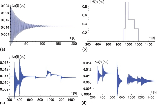

b) The results based on Mathematica are shown in Figures E11.11.3. The Mathematica input program is listed in Table E11.11.1.
11.4.7 Power Quality Issues Due to Renewable Sources
In addition to power-load balance issues, distributed renewable sources lead to high system impedances at the distribution level because these plants cannot deliver additional transient currents when faults occur due to their operation at peak power [68]. Even with acceptable current harmonics, this high system impedance may result in unacceptably high voltage harmonics, single-time events (e.g., spikes due to network switching and synchronization) and non-periodic but repetitive (e.g., flicker) events, and contribute to power quality problems [160–162,46–48,50].
The frequency/load control in distributed grids with a majority of renewable sources (e.g., renewable generation larger than 50%) appears to be the most difficult part of a smart grid and requires extensive research. In addition the transfer of power via AC and DC lines --associated with harmonic and power factor control--must be studied: most necessary software programs, e.g., symmetric (based on single phase) and asymmetric power (based on three phases) flow programs for this effort are available for integer harmonics, but are not available for sub and non-integer harmonics.
11.4.8 Control of Voltage and Reactive Power
Today frequency and voltage control predominantly occurs at the AC transmission level. In distributed systems with renewable sources these control functions will take place both at the transmission and distribution levels. As the intermittency of renewable sources makes frequency and voltage control more difficult, short- and long-term storage plants for electric energy must be relied on to compensate the energy flow [163]. This involves an increase of switching actions which may impair the quality of energy delivered to the consumer.
11.4.8.1 Transition from Central Power Station to Distributed Energy Sources
The problems which may arise due to the transition from central power stations to distributed energy sources are detailed for Germany. Depending upon the operating levels, 26 nuclear plants supplied in 2005 about 25–42% of the energy while renewable sources provided only 14% and hydro plants supplied about 3-7% [164]. Recent decision of phasing out [165] nuclear power put tremendous pressure on government to scale up renewable sources in the transmission and distribution system. According to Steininger [166], in 2011 “green energy” accounted for more than 20% for the first time and it is predicted to reach 35% by 2020. How can the grid accommodate such a relatively high percentage of intermittently operating sources without sacrificing network stability and supply reliability?
A recent article [167] indicates that the German grid might be stressed (e.g., large frequency and voltage deviations) even at light-load conditions if the 26 nuclear plants are permanently disconnected. Distributed central stations (nuclear, coal and natural gas) ensure that the power-flow control is relatively stable because energy cannot be transmitted over long (e.g., 800 km) lines to reach the consumer. These interconnected grids maximize stability, efficiency and reliability while minimizing investment costs. Decommissioning nuclear plants and minimizing the operation of coal-fired plants limits generation to intermittently operating sources, natural-gas- fired and a small percentage of hydro plants. While natural-gas-fired plants generate less CO2 than coal-fired plants, they rely on methane, and the leak thereof increases global warming much more than CO2. The National Center for Atmospheric Research (NCAR) in Boulder, Colorado estimates that natural-gas wells leak about 10% of their production capability [168]. In Germany, the fact that wind-power (WP) plants are predominantly located in the North (offshore in the North Sea) and PV plants are mainly located in the South means that the electric energy must be transmitted over a long distance (about 800 km) resulting in unacceptably large frequency and voltage perturbations [167], which lead to stability problems due to large transmission-line impedances and switching actions. This is why the technical community strongly advocates [169] construction of additional 3,800 km of new power lines until 2025 [170]--of which DC current lines will account for 2100 km and AC lines for 1700 km--stretching from the Baltic and North Sea to the South of Germany, respectively. The construction of large short- and long-term storage plants must accompany renewable sources [1,64,171]. To minimize stability problems of AC lines, extra-high-voltage (EHV) e.g., 735 kV are required if generating stations and loads are very far apart [167,49], reducing the per-unit line impedance and maximizing the transmission-line section length for which stability can be maintained. Special problems arise that require compensation equipment, e.g., synchronous capacitors, inductive reactors, static VAr compensators, shunt and series capacitors, and flexible AC transmissions (FACTS) [172] to control voltage and assure stability of energy transmission.
If high-voltage DC lines are employed no voltage instability will occur--this is the advantage of DC lines. However, stability problems due to mismatch of generation and consumption still occur and storage plants cannot be dispensed with in the latter case as well. The following sections focus on the stress (e.g., large frequency variations, instability) in transmitting power from distant renewable sources to load centers via AC lines. The development of the AC transmission-line infrastructure will become important in addition to the design of renewable sources and strategically located large storage plants [167,1,64,171].
At light load (to fully utilize renewably generated energy) most central power stations such as coal and natural-gas-fired plants will be operated at reduced levels. For example, wind energy from the North of Germany will be transmitted via 800 km EHV-AC line to the South if there is not much insolation, and vice versa, if there is not much WP available. Note that outputs of PV and WP plants change rapidly (Figure 5 of [64]). In this case the AC power system might be stressed from a frequency and reactive power point of view.
11.4.9 Frequency Variations Due to Charging and Discharging of Storage Plants of Grid with Renewable Sources
The objectives of operation of the grid with renewable sources and storage plants where a natural-gas-fired plant is the frequency leader are:
1) Modeling of an AC power system with renewable sources and storage plants and its frequency variation due to switching actions, if energy is transmitted from renewable sources to load centers 800 km away with and without energy storage plants [49];
2) Determination of length of AC transmission line sections to ensure steady-state and dynamic stability;
3) Selection of time constants of conventional, renewable, and storage plants;
4) Operation of WP and PV plants and charging and discharging of energy storage plants must be such that the transmission line power changes only gradually. Frequency control within acceptable limits (49-51) Hz [159] can be achieved by compensating/complementing the output of PW and PV plants with those of storage plants.
11.4.9.1 Simplified Grid
Figure 11.29 illustrates a simplified AC grid [49] with predominantly renewable energy sources: WP farm in the North of Germany and associated short-term storage plant to compensate for the intermittent output of wind farm. Natural-gas and long-term storage plants are used for peak-power generation near the two load systems. In the South there is a PV farm with associated storage plant. Figures 11.30a, b depict the frequency control for either storage-plant operation or renewable-source operation. In Figure 11.30a the WP and PV plants have no output power and the short-term storage PV and WP plants together with the natural-gas fired plant control though appropriate droop characteristics the frequency of the AC power system. In Figure 11.30b the PV and WP plants operate at their maximum output power through peak-power tracking together with the natural-gas fired and long-term storage plants while the PV and WP storage plants have zero output. There are three modes of operation:


Mode #1: renewable sources (RS) and storage plants supply power to two load systems.
Mode #2: RS charge storage plants [144].
Mode #3: RS supply energy to two load systems.
If the transmitted power throughput across the AC transmission line is not changing slowly enough, frequency stability problems set in due to discontinuous AC power transmission and associated frequency perturbations. For example, a three-phase, 735 kV (line-to-line), 50 Hz, 800 km line has a reactance of 0.55 Ω/km [173] or XL = 440 Ω resulting at base apparent power S = 1000 MVA with the base impedance of Zbase = (735)2/1000 = 540 Ω in a per-unit line reactance of XLpu = (440/540) = 0.815pu. With a transformer reactance of XTpu = 0.08pu the total line reactance is Xtotal = XLpu + 2XTpu = (0.815 + 0.16)pu = 0.98 pu @ 50 Hz. Transient analysis shows that this long AC transmission line will have to be subdivided into about five sections each having a per-unit reactance of Xsection = Xtotal/5 = 0.98/5pu = 0.196 pu, and at the terminals of each section the voltage will have to be controlled to guarantee stability of transmission. The differential and algebraic equation system of Figure 11.29 is listed below. The AC transmission/tie line acts as an integrating component [144] enforcing Δω(s) = Δω1(s) = Δω2(s). The differential and algebraic equations are solved with Mathematica software; s is the Laplace operator.
System #1:
Coupling (tie, transmission) network:
System #2:
System #3:
System #4:
System #5:
System #6:
11.4.9.2 Limits on Stability of Transmission
Wind energy from the North to the South of Germany can be transmitted with EHV AC lines divided into five sections: one section has the per-unit reactance of Xsection = 0.196 pu. Two scenarios are investigated: first (mode #1) when the WP plant, load ref3(s), and its associated storage plant, load ref4(s), are supplying power via AC transmission line T/s to the two load systems, during which time the natural-gas-fired plant supplies load ref1(s) = 0.8 pu power and the long-term storage plant supplies load ref2(s) = 0.4 pu power to the two load systems defined by M1, M2, D1, D2, ΔPL1(s), ΔPL2(s) [49]. The time constants of the various plants (e.g., TCHi for i = 1 to 6) influence the stability of AC transmission. The input parameters load ref1(s) to load ref4(s) and [-ΔPstorage4(s)], as defined in Figure 11.29, are positive and their values depend on the power gains of the plants. Note, load ref1(s) must be nonzero because the natural-gas-fired plant is the frequency leader.
11.4.9.3 Non-Constant Power Output of Renewable Sources
Mode #1: Figures 11.31a-d show that at Xsection = 0.196 pu at large-step outputs of WP plant and associated storage plant permit a stable AC energy transmission to the two load systems in the South, defined by M1, M2, D1, D2, ΔPL1(s), ΔPL2(s) [49]. However, the angular frequency variations due to switching are large (0.25pu). At Xsection_max = 0.33 pu instability sets in as indicated in Figure 11.32 where load ref5(s) = ΔPstorage6(s) = 0. Reduced time constant TCH1 = 1.4 s results in the stability as demonstrated in Figure 11.33. For medium-step outputs of WP illustrated in Figure 11.34a and associated storage plant the frequency variation due to switching is still large (0.07 pu), as indicated in Figures 11.34b, c. Best performance with lowest angular frequency variation due to switching (0.01 pu) is obtained with small-step outputs of WP (as shown in Figure 11.35a) and associated storage plant, as depicted in Figures 11.35b, c; however, instability results for Xsection = 0.33 pu as indicated in Figure 11.36.


Mode #2: If the WP plant large-step output (load ref3(s) ≠ 0, ΔPstorage4(s) = load ref3(s)) charges the associated short-term storage plant ΔPstorage4(s) large (0.05 pu) angular frequency variations of Figure 11.37a are obtained while the transmission tie line power (neglecting switching transients) is about constant as depicted in Figure 11.37b. For small-step charging the angular frequency variation is smaller: 0.02 pu, see Figure 11.38a and the tie line power as given in Figure 11.38b is about constant and shows smaller transient excursions during switching. The spikes in the Δω(t) = Δω1(t) = Δω2(t) are mitigated by smoothing the output of the WP plant based on small-step operation. The AC transmission of energy from the South PV farm to the two load circuits in the North is similar as discussed above.


According to the newspaper [169] “Financial Times Deutschland”, DC transmission lines are planned [170] to avoid stability problems associated with long AC lines and result in smaller line voltage drops (no reactive drop). DC lines could be mounted on existing towers/pylons presently used for AC transmission lines to reduce costs and avoid protests by citizens. Although DC lines solve the voltage stability problem associated with AC lines, DC lines still require short-term and long-term storage to control the frequency at the AC load side by enforcing power balance. DC lines are known for their voltage distortions, thus harmonic filters would also be required as discussed in Chapter 9. Frequency control can be achieved by employing short-and long-term storage plants [1,144] complementing output of renewable sources by small step-wise control of the AC transmission-line power. Stable AC transmission results by appropriate power management: wave shaping of power inputs/outputs, appropriate transmission line segmentation, and selection of power plant and storage plant time constants.
11.4.10 Reduced Life Time of Storage Plants
Renewable sources as well as all types of storage plants are operated intermittently, and therefore the winding structures of generators are thermally exposed to changing temperatures through changing loss and heating conditions: this causes the winding to contract and expand depending upon the changing temperature resulting in mechanical degradation (see Chapter 6) of the insulating material of electrical components such as generators (Chapter 4). The rated lifetime of about 40 years is thus reduced by a factor of two resulting in long outages (e.g., half a year) of plants.
11.4.11 Solutions to Power Quality Problems Due to Renewable Plants with Energy Storage Systems
Frequently charging and discharging of storage plants impact the lifetime of the insulation material due to mechanical stresses and temperature changes. In addition the transients due to rapid frequency changes induce mechanical (e.g., flywheel) and electrical (e.g., overvoltage) stresses in the equipment. To operate storage and renewable sources in a complementary stable manner the droop characteristics must be different where the small-sloped characteristic is associated with the frequency leader. In addition the control of storage and renewable sources must have sufficient gains and small enough time constants as required by fast mechanical [174] and electronic valving and switching, respectively. Parameter variations are an important subject in the field of power quality because these may cause instability of the grid.
11.5 AC transmission lines versus DC lines
In the past mostly AC transmission lines have been used, except for DC underwater cable transmission applications. The occurrence of ferroresonance (see Chapter 2) limits the length of AC cables above 20 kV. In addition there exists a stability problem for AC lines longer than about 1000 miles. For this reason high-voltage DC transmission lines have been used in Scandinavian countries [175] and in California [176]. DC lines have several advantages (use of less copper because there is no skin effect, no stability problem at any transmission line length) and disadvantages (the need for converter stations on both ends of the line, the generation of harmonics on the AC and DC sides due to rectification and inverter action).
11.5.1 Solutions to Power Quality Problems of High-Voltage AC Transmission Lines
The problem with buried AC transmission lines is that at voltages larger than 20 kV at a certain length ferroresonance sets in due to the large cable capacitances. This is the reason why at high voltages, overhead lines are installed which have small network capacitances. Gas-filled cables – avoiding ferroresonance-- have a reduced capacitance and can be buried. However, gas-filled cables are very expensive. DC transmission lines do not experience ferroresonance, and can be either overhead or underground lines. The application of rectifiers and inverters complicate their application at large transmission power ratings, say 2,000 MW.
11.6 Fast-charging stations for electric cars
The large-scale introduction of electrical automobiles hinges on the two important issues: mileage range and fast charging of (heavy) batteries. If the weight of transportation vehicles such as cars and air planes is reduced, then their energy consumption can be either reduced or their mileage can be increased based on the figure of merit (FM) relation [1]

In particular the use of carbon [177] fiber and aluminum will decrease the weight in addition by replacing mechanical gears with electric gears so that the mileage range of electric cars can be at least 350 km [178]. For example, the BMWi3 [179] with a carbon-fiber passenger cell and an aluminum-drive module has at a curb weight of 1.2 tons-force, a mileage of 100 miles per battery charge of 22 kWh resulting in the figure of merit FM = (1.2tons-force)·(100 miles)/(22kWh) = 5.45.
11.7 Off-shore renewable plants
Over the course of the past decade, the development of off-shore WP has skyrocketed. Back in 2000, a meagre 36 MW was installed around the world, a figure which has grown rapidly ever since. By the end of 2012, the cumulative installed capacity of off-shore wind farms had reached an impressive 5,410 MW. The move to offshore wind energy gained serious traction in 2010 when 999 MW were added across the world. In 2011 and 2012, this figure grew to 1,033 and 1,292 MW respectively [180–182].
11.8 Metering
There are two types of electricity metering: net-metering and feed-in tariff metering [1].
11.8.1 Net Metering
Most electricity meters are bi-directional and can measure current flowing in two directions [1]. This permits one to easily bank excess electricity from your solar panels for future credit. Net metering only requires one power meter, while feed-in tariffs require two. Unlike feed-in tariffs and power purchase agreements, the credits one accumulates through net metering are always at full retail value. Net metering was first adopted by utilities in Idaho in 1980. Since the Energy Policy Act of 2005, every public electric utility in USA is required to offer net metering to their customers.
11.8.2 Virtual Net Metering
Virtual net metering is basically net metering (with one electric meter) shared between several people. This enables homeowners that are unsuited for solar for one reason or the other, to participate in community-owned solar farms (also known as solar gardens). There are about one dozen virtual net metering systems operating in the U.S. at the time of writing.
11.8.3 Feed-In Tariff
Feed-in tariff requires one extra power meter in order to measure outflow of electricity from your home independently. This enables electricity consumption and electricity generation to be priced separately as is done in Germany by Stadtwerke München (SWM) and most other utilities. Feed-in tariff schemes are typically based on a 15-20 yearlong contract where prices are pre-defined above retail with a tariff that is subject to changes, either by regular degression or by legislative changes, which effectively reduces your earnings over time. For every kWh one generates one gets paid. Only six states across the U.S. currently have some form of feed-in tariff scheme as of today: California, Florida, Vermont, Oregon, Maine, and Hawaii.
11.9 Other renewable energy plants
Ocean-tide plants are investigated in France and in the United Kingdom, where the tides and the geological formations lend themselves to such energy sources. The groundwater heat pump again depends upon the geological formations and is used in Application Example 11.1. The idea of capturing electrical energy from geomagnetic fields has been researched, but no practical applications have come forward because it is very difficult to use high frequency to beam the energy from space to earth. The same problem exists with beaming the energy from space to earth, if PV arrays generate electricity in space [183]. The recovery of braking energy in automotive applications is used [1] for hybrid electric cars and for electric trains. About 10-20% of the energy can be recovered for short-distance travel. For long-distance travel this percentage will be much smaller. The utilization of methane emanating from garbage dumps is relied on in few cases only. With the recycling of compostable material this type of methane collection will not play a major role. Although the Stirling engine [184] has been known for a long time, no feasible applications have been introduced to date. Depending upon the geological formation geothermal energy can be utilized: the center of the earth has a temperature of about 5,000 to 6,000 ° C. This stored heat originating in the natural radioactive decay streams to the surface layer of the earth and heats rocks and groundwater, as is illustrated in Figure 11.39. The Aschheim/Feldkirchen/Kirchheim AFK [185] geothermal company near Munich utilizes this natural geothermal energy. It is expected that the temperature gradient is approximately 3.2 ° C per 100 m depth. Near Munich these heat energies can be accessed fairly easily because of the limestone containing water (Figure 11.39). These layers contain at a depth of about 2,200 to 2,700 m warm water with a temperature of 85 ° C. Co-generation plants where electricity generation, and warm/cooling water production are combined are frequently installed [1] on university campuses, municipalities, and industrial production facilities.

In contrast to the solid electrolyte fuel cells (SOFC) with a few tens of MW electrical output, the three thermal combined heating and electric power (CHP) --fed by a combination of conventional fuel with biomass, refuse/garbage--plants in Munich (North-, South-, and Freimann plants) [186] deliver a total of 1,269 MWe (where e means electric) and a heating power of 1,998 MW by meeting all required environmental pollution regulations, supplying 58% of the electric power consumed in Munich with the maximum efficiency of 90%, if heat and electric power outputs are at their rated values.
11.10 Production of automotive fuel from wind, water, and CO2
High-temperature electrolysis at 800 degrees Celsius has an efficiency of over 90% [187], where the input consists of electricity and water yielding from (water) steam in a first step hydrogen and oxygen gases. In a second step the hydrogen gas and carbon dioxide results in synthesized fuel for automotive applications which can be mixed with gasoline, diesel or jet fuel. The overall efficiency of this two-step process is about 70%. This process uses for each ton-force generated synthesized fuel about 3.2 tons-force of CO2 taken from the air. It is estimated that one liter of this synthesized fuel costs about 1.3 Euro. Car manufacturers indicate that for any percentage mix of synthesized fuel with either gasoline or diesel no changes in the car engine technologies will be required. In addition the synthesized fuel will neither contain sulphur nor nitric oxides, and no food supplies (e.g., corn) will be used for this synthetic fuel production.
11.11 Water efficiency
One way to boost water efficiency is to promote the use of more technologically advanced controllers so that residential and commercial landscape irrigation moves beyond the currently predominant techniques of manual irrigation or conventional automatic timers. Results [188] suggest that wider adoption of advanced irrigation control technologies would result in average water savings that could lessen the strain on aging water treatment infrastructure and on overtaxed freshwater resources.
11.12 Village with 2,600 inhabitants achieves energy independence
In 1999 the village council of Wildpoldsried, located in Bavaria, Germany decided to take with the mission statement WIR (Wildpoldsried Innovative Redirecting) a lead with respect to renewable energy [189–192]. Based on this motto, with the participation of citizens, an ecological profile was developed that was distinguished by regional, Bavarian and international administrations and societies due to its innovativeness and leadership. For example, in April 2000 two wind power (WP) plants with 1 MW each were installed with the financial support of 30 citizens. Subsequently, 93 citizens financed in December 2001 two 1.5 MW WP plants, in October 2007 one 2 MW WP plant was constructed based on support of 60 citizens, and finally 99 citizens financed two 2.3 MW WP plants. This exemplary engagement of 282 citizens resulted in 7 WP plants with a total of 11.6 MW installed output power capacity.
The pilot research project [189,190] for the “Integration of Renewable ENergy and Electro-mobility” (IRENE) in Wildpoldsried started in 2011 in order to demonstrate for two years--based on decentralized intermittently operating renewable energy sources such as photovoltaic, wind, and biogas power plants--economic solutions for the local utility Allgäuer Überlandwerke GmbH. One important component is the self-organizing, real-time energy control system designed by Siemens AG. Another component is the measuring of parameters at more than 200 locations of the decentralized distribution system in order to optimize intermittent generation, consumption, and storage of electric energy. For 8 months 30 electric vehicles were available to citizens for test-mode operation and partly were used as storage components to charge and discharge within the smart-grid environment in order to mitigate the peaks of generation and consumption. Additional contributors to this exemplary project are Hochschule Kempten and RWTH Aachen. Figure 11.40 shows the consumption and generation of renewable energy in Wildpoldsried in 2013 measured in MWh. The 6,480 MWh represent electricity consumption without supplying it to heating systems such as storage heaters or heat pumps. Biogas is generated based on liquid manure supplied by seven local farmers, including silage, dung, and foodstuffs such as onions, potatoes, and corn that have spoiled and are not suitable for human consumption. The distribution system is not self-sufficient ---that is, it is not a micro grid-- because it is always connected to the local utility grid.

11.13 Summary
The size and number of renewable energy sources can be minimized through their efficient use: an energy unit saved means it does not need to be generated by renewable sources. Frequently inexpensive electronic devices/components have the highest efficiency, but poor power quality: examples with respect to steady-state operation are peak rectifiers, power electronic heating elements based on burst-voltage/current and phase-angle voltage/current control for induction-type stoves generating sub-, non-integer, and integer harmonics. Any power electronic switching involves snubbers, reverse-recovery currents, differential and common-mode noise which must be eliminated through appropriate filters. Other examples are permanent-magnet machines operating either in full-on or pulse-width-modulation (PWM) mode. In the full-on mode the efficiency is higher than that at PWM. However, the power quality at full-on mode is poor due to current harmonics generated by the driver/inverter circuit. PV and WP plants operate mostly under non-steady state and transient operation requiring maximum-power point operation, short-term and long-term storage components in addition to filters to provide for the consumer a constant frequency and voltage at an acceptable power factor and quality. This relates to the efficiency of transmission: a low power factor increases the losses within a transmission line.
This chapter includes practical examples (e.g., measuring the PV output power of residence, Figure E11.1.1, and its total electrical generated powers, Figure E11.1.3, measuring the performance of electronic gear, Figures 11.14 to 11.16) and theoretical (PSpice and Mathematica solutions) considerations of power quality solutions for renewable energy systems. Additionally 11 practical application examples with 23 hands-on problems at the end of the chapter and 192 references relate the topics to real world problems. The operation of PWM rectifiers and inverters is explained based on PSpice program. Frequency control as a function of short- and long-term storage elements is analyzed with Mathematica. It appears that for the consumer the net-metering approach is more advantageous than the feed-in tariff approach. In the first case the grid is used as storage of electric energy which can be recalled during times when the PV plant does not generate sufficient energy for the residence. In the feed-in approach the utility pays for the delivered kWh only about half or less what the consumer pays for the kWh bought from the utility. This chapter discusses the most important renewable energy sources and their impact on power quality. Less popular renewable sources are summarized at the end of the chapter. Most renewable energy sources require a detailed knowledge of power quality solutions.
11.14 Problems
Problem 11.1: Design of Photovoltaic (PV) Power Plant for Residence
A PV power plant consists of solar array, peak (maximum)-power tracker [1], a step-up/step-down DC-to-DC converter, a deep-cycle battery for part f) only, a single-phase inverter, single-phase transformer, and a residence requires a maximum inverter AC output power of Pinvmax = 5.91 kW as shown in Figure P11.1.1. Note, the maximum inverter output AC power has been specified because the entire power must pass through the inverter for all operating modes as is explained below. In addition, inverters cannot be overloaded even for a short time due to the low heat capacity of the semiconductor switches.

Three operating modes will be investigated:
1) in part f) the operating mode #1 is a stand-alone configuration (546 kWh are consumed per month in Munich, Germany)
2) in part g) the operating mode #2 is a configuration, where the entire energy (546 kWh) is consumed by the residence and the utility system is used as storage device only,
3) in part h) the operating mode #3 is a configuration, where 60 kWh are consumed by the residence and 486 kWh are sold to the utility. The consumption in the residence -- disregarding heating energy -- is low due to LED lighting, high efficiency appliances (e.g., refrigerator, induction-type stove), and electronic equipment
a) The power efficiencies of the maximum power tracker, the step-up/step-down DC to DC converter, the battery, and the inverter are 97% each, while that of the transformer is about 1.00. What maximum power Pmaxsolararray must be generated by the solar plant (array), provided during daytime Emonth_day = 60 kWh will be delivered via the inverter to the residence (without storing this energy in battery), and sufficient energy will be stored in the battery so that the battery energy of Emonth_night = 486 kWh can be delivered during nighttime by the battery via the inverter to the residence: that is a total of Emonth = Emonth_day + Emonth_night = 546 kWh can be delivered to the residence during one month?
b) For a commercially available solar panel the V-I characteristic of Figure 3.23 of [1] was measured at an insolation of Qs = 0.9 kW/m2. Plot the power curve of this solar panel: Ppanel = f(Ipanel).
c) At which point of the power curve Ppanel = f(Ipanel) would you operate assuming Qs = 0.9 kW/m2 is constant? What values for power, voltage and current correspond to this point?
d) How many solar panels would you have to connect in series (Ns) in order to achieve a DC output voltage of ![]() 480 V of the solar plant (array)? How many solar panels would you have to connect in parallel (Np) in order to generate the inverter output power Pinvmax = 5.91 kW?
480 V of the solar plant (array)? How many solar panels would you have to connect in parallel (Np) in order to generate the inverter output power Pinvmax = 5.91 kW?
e) How much would be the purchase price of this solar power plant, if 1 kW installed output capacity of the inverter (this includes the purchase costs of solar cells + peak-power tracker + DC-to-DC converter + inverter) costs US $3,500 (without utility rebates and state/federal government tax-related subsidies)?
f) Operating mode #1
What is the payback period (in years, without taking into account interest payments) of this solar plant if you use in your residence 546 kWh per month at an avoided cost of US $0.37/kWh (includes service fees and tax)? (You may assume that this solar plant can generate every month 546 kWh and there is no need to buy electricity from the utility: 60 kWh per month will be used in the residence during daytime and during nighttime 486 kWh per month will be supplied via inverter from the battery to the residence). However, there is a need for the use of a 20 kWh deep-cycle battery as a storage element so that electricity will be available during hours after sunset. This battery must be replaced every four years at a cost of US $4,000.
g) Operating mode #2
What is the payback period (in years, without taking into account interest payments) of this solar plant if you use in your residence 60 kWh per month at an avoided cost of US $0.37 per kWh? You may assume that this solar plant can generate every month 546 kWh and every month the solar plant feeds 486 kWh into the power system of the utility company which reimburses you US $0.22 per kWh (so-called “net metering”, see reference 27 of Chapter 1 [1]). In this case there is no need for a battery as a storage element because during the hours after sunset the electricity can be supplied by the utility: 486 kWh at US $0.22 per kWh. There is a connection charge of US $7.00 per month.
h) Operating mode #3
What is the payback period (in years, without taking into account interest payments) of this solar plant if you use in your residence 60 kWh per month at an avoided cost of US $0.37 per kWh? You may assume that this solar plant can generate every month 546 kWh of which every month the solar plant feeds 486 kWh per month into the power system of the utility company which reimburses you US $0.22 per kWh. There is a connection charge of US $7.00 per month.
i) Which power plant configuration (e.g., f, g or h) is more cost effective (e.g., has the shortest payback period)?
j) What is the total surface of the solar panels provided the efficiency of solar cells is 15% at Qs = 0.9 kW/m2?
k) Instead of obtaining tax rebates and state/federal government subsidies the owner of a PV power plant obtains a higher price (feed-in tariff, see Chapter 1 [1]) for the electricity delivered to the utility: Provided 546 kWh are fed into the utility grid at a reimbursement cost of US $0.22/kWh and the utility supplies 60 kWh to the residence at a cost of US $0.37/kWh, what is the payback period if the entire plant generating 5.91 kWAC (there are no batteries required for storage) costs US $24.355 k. You may neglect interest payments, and there is a connection charge of $7.00 per month.
l) Repeat part k) taking into account interest payments of 2.85%.
Problem 11.2: Calculation of Energy Consumption in Residence per Living Space (m2) and per Year (a)
A residence with 300 m2 finished living space requires 12,000 kWh of energy (input/consumption in house) during one year. Determine the energy consumption in house per square meter and per year.
Problem 11.3: Photovoltaic (PV) Energy Yield as a Function of Latitude
Calculate based on the National Renewable Laboratory (NREL) software available at http://rredc.nrel.gov/solar/calculators/PVWATTS/version1/ the electric energy generation for a PV residential plant of 6.48 kW installed output power capacity when either located at a latitude (array tilt) 40.02 degrees (e.g., Boulder Colorado, cost of electricity is US$ 0.16/kWh) and at latitude (array tilt) 48.13 degrees (e.g., Munich Germany cost of electricity is 0.26 Euros/kWh = US$ 0.36/kWh) in the northern hemisphere for an array azimuth of 180 degrees with an overall DC to AC derating (electrical efficiency of all components) factor of 0.77 and an array type 20 degree tilt in Boulder and an array tilt of 48.13 degrees in Munich.
Problem 11.4: Burst-Current/Voltage Control for Induction-Type Stove/Cooker
An induction-type stove has a rated power of Prat = 800 W with (Ton/T) = 0.8 at 50 Hz find the output heating power of the induction-stove coil. Normally burst-current control relies on the frequency range 20-50 kHz, but in this problem 50 Hz are chosen for simplicity.
Problem 11.5: Burst-Current/Voltage Control for Induction Stove/Cooker
An induction-type stove has a rated voltage of Vt_rms_rat = 240 V at f = 50 Hz with (Ton/T) = 0.8 find the input voltage of the induction-stove coil. Normally burst-current control relies on the frequency range 20-50 kHz, but in this problem 50 Hz are chosen for simplicity.
Problem 11.6: Current Harmonics Injected into Power System by Burst-Current Control
It can be assumed that for burst-voltage control, current and voltage are in phase because of resistive load Rload, and both have sinusoidal wave shapes. Assume a burst period of T = Ton + Toff, where Ton/T = 0.5 at f = 50 Hz for sinusoidal terminal voltage with Vt_rms_rat = 240 V. Normally burst-current control relies on the frequency range 20-50 kHz, but in this problem 50 Hz are chosen for simplicity.
a) What are the firing angles of the two thyristors of Figure E11.2.2a for Ton/T = 0.5?
b) Write a PSpice program for circuit of Figure E11.2.2a and compute the current through Rload = 2.2 Ω of Figure E11.2.2a.
c) Determine the Fourier coefficients of the current through Rload up to the 21th harmonic.
d) Plot the current through Rload together with the terminal voltage V(10)-V(0).
e) What types of current harmonics are generated in I(Rload):
(2) inter-harmonics/fractional harmonics/non-integer harmonics,
(3) integer harmonics?
Problem 11.7: Phase-Angle Current Control for Induction Stove/Cooker
An induction-type stove has a rated voltage of Vt_rms_rat = 240 V at f = 50 Hz with (tdelay/T/2) = 0.4 find the input voltage of the induction-stove coil. Phase-angle current control relies sometimes on a higher frequency than 50 Hz, but in this problem 50 Hz is chosen for simplicity.
Problem 11.8: Current Harmonics Injected into Power System by Phase-Angle Current Control
It can be assumed that for phase-voltage control the load is resistive as indicated in Figure E11.2.2a and the voltage has sinusoidal wave shape. Compute the phase current through load resistor Rload = 2.2 Ω as shown in Figure E11.2.2a for a sinusoidal terminal voltage with rms value Vt_rms = 240 V and a current phase angle delay time tdelay = 3 ms at f = 50 Hz. Phase-current control relies sometimes on a high frequencies (20-50 kHz), but in this problem 50 Hz are chosen for simplicity.
a) What are the firing angles of the two thyristors of Figure E11.2.2a for tdelay = 3 ms?
b) Write a PSpice program for circuit of Figure E11.2.2a and compute the current through Rload of Figure E11.2.2a.
c) Determine the Fourier coefficients of the current through Rload up to the 21th harmonic.
d) Plot the current through Rload together with the terminal voltage V(10)-V(0).
e) What types of current harmonics are generated in I(Rload):
(2) inter-harmonics/fractional harmonics/non-integer harmonics,
(3) integer harmonics?
Problem 11.9: PWM Rectifier Output Voltage VDC load = V(Rload) = f(Vrms) at Constant Duty-Cycle δ for Variable Input Phase Voltage Vrms
Section 11.2.4.1 computes for a pulse-width-modulated (PWM) three-phase rectifier the dependency of the input voltage VaN max at a constant output voltage VDC load and constant output current IDC load provided the duty cycle δ is variable.
In this problem compute and plot for the rectifying circuit of Figure 11.1 the input phase currents I(VaN), I(VbN), I(VcN), and output voltage VDC load = V(Rload) as a function of the input phase voltages VaNmax, VbNmax, VcNmax = √2Vrms = (233 V, 465 V, 930 V) at a constant duty cycle δ = 0.50 from 300 ms to 325 ms. The PSpice program of Table 11.1 can be used as a starting point with switch gating signal frequency = 20 kHz.
Problem 11.10: PWM Rectifier Output Voltage VDC load = f(δ) for Constant Input Voltage Vrms = 329 V
Section 11.2.4.1 computes for a pulse-width-modulated (PWM) three-phase rectifier the dependency of the input voltage VAN max at a constant output voltage VDC load and constant output current IDC load provided the duty cycle δ is variable.
In this problem compute for the rectifying circuit of Figure 11.1 the output voltage VDC load as a function of the duty cycle δ at constant input voltage Vrms = 329 V, where the input sinusoidal phase-voltage amplitude is VaN max = 465 V. The PSpice program of Table 11.1 can be used as a starting point.
Problem 11.11: Current-Controlled PWM Inverter Output Voltage Vrms = f(VDC) for Given Modulation Index m
Section 11.2.4.2 computes for a current-controlled pulse-width-modulated (PWM) three-phase inverter the dependency of the input voltage VDC at constant output voltage Vrms l-n as a function of the displacement (power factor) angle φ and the modulation index m.
In this problem compute the output currents Irms ph and the modulation index m of the inverter circuit of Figure 11.6a, b for the output voltages Vrms = (240/√3) V = 139 V, (380/√3) V = 220 V, (480/√3) V = 277 V as a function of the input DC voltage VDC = 700 V for leading, lagging and unity displacement (power) factors (generator notation) with displacement power factor angle φ. The PSpice program of Table 11.3 can be used as a starting point with switch gating signal voltage (vtrial) frequency of 17.28 kHz.
Problem 11.12: Current-Controlled PWM Inverter Output Voltage Vrms = f(m) for Given Input Voltage VDC
Section 11.2.4.2 computes for a current-controlled pulse-width-modulated (PWM) three-phase inverter the dependency of the input voltage VDC at constant output voltage Vrms l-n as a function of the displacement (power factor) angle φ and the modulation index m.
In this problem compute for the inverter circuit of Figure 11.6a, b the modulation index m for constant input DC voltage VDC = 400 V and variable output inverter phase voltages Vrms ln (240/√3 = 139 V, 380/√3 = 220 V, 480/√3 = 277 V, 600/√3 = 346 V, 2400/√3 = 1386 V) at unity power factor. The PSpice program of Table 11.3 can be used as a starting point. The frequency of the gating signal voltage is 5.76 kHz.
Problem 11.13: Differential-Mode Electrical Noise Filter
The differential electrical noise of f10kHz = 10 kHz with the amplitude of ![]() across the terminals of a VDC = 12 V power supply for a radio must be attenuated to Vnoise = 10 m V. Figure P11.13.1 shows the circuit of the battery voltage of VDC = 12 V including the
across the terminals of a VDC = 12 V power supply for a radio must be attenuated to Vnoise = 10 m V. Figure P11.13.1 shows the circuit of the battery voltage of VDC = 12 V including the ![]() as well as the differential-mode filter with impedance Zfilter = Rfilter + 1/(j2π·f10kHz·Cfilter). You may assume Rfilter = 0.1Ω, Zbattery ≈ Rbattery = 0.5 Ω, and Rradio = 1 Ω.
as well as the differential-mode filter with impedance Zfilter = Rfilter + 1/(j2π·f10kHz·Cfilter). You may assume Rfilter = 0.1Ω, Zbattery ≈ Rbattery = 0.5 Ω, and Rradio = 1 Ω.

a) Draw the AC circuit of Figure P11.13.1.
b) Compute the required capacitance Cfilter of the filter.
Problem 11.14: Common-Mode Electrical Noise Filter
The internet connection of a computer is from the modem 20 m long, and the transmission is frequently interrupted due to common-mode noise. Design a suitable filter and specify its components to reduce the maximum value of the common-mode current to icommon = 10 μA.
Problem 11.15: Maximum Power Point of a PV Array of a Pout = 8 MWAC Photovoltaic (PV) Power Plant
A PV power plant consists of solar panels, peak-power tracker, step-down/step-up DC-to-DC converter(s) (20 connected in parallel), three-phase inverter(s) (20 connected in parallel), Y-Δ three-phase transformer, and a three-phase power system absorbing the rated (nominal) output power Pout inverter of the 20 inverters at rated operation and rated (maximum) insolation Qs = 0.9 kW/m2. The block diagram of this plant is shown in Figure P11.15.1. The power efficiencies of the peak-power tracker, step-down/step-up DC-to-DC converters, inverters, and transformer are η = 95% each.

a) Using the output characteristics of the solar array of Figure P11.15.2a determine at an insolation of Qs = 0.9 kW/m2 the output (peak) power of the solar array ![]() , and the resulting output power of the 20 parallel-connected inverters
, and the resulting output power of the 20 parallel-connected inverters ![]() .
.

b) If the line-to-line voltage of the power system -which is identical to the output line-to-line voltage of the Δ-secondary of the Y-Δ transformer (t)- is ![]() = 13.2 kV determine the input line-to-line voltage of the Y-primary of the transformer -which is identical with the output line-to-line voltage of the 20 (parallel-connected) inverters (i)
= 13.2 kV determine the input line-to-line voltage of the Y-primary of the transformer -which is identical with the output line-to-line voltage of the 20 (parallel-connected) inverters (i) ![]() - provided the DC input voltage of one inverter is VDCi= 2 kV and the modulation index m = 0.8, see modulation index m for inverters in [1, Chapter 5]. What is the turns ratio of the transformer Np/Ns where the primary (p) is the Y-winding and the secondary (s) is the Δ-winding of the Y-Δ transformer, see 3-phase transformer connections in [1, Chapter 8]?
- provided the DC input voltage of one inverter is VDCi= 2 kV and the modulation index m = 0.8, see modulation index m for inverters in [1, Chapter 5]. What is the turns ratio of the transformer Np/Ns where the primary (p) is the Y-winding and the secondary (s) is the Δ-winding of the Y-Δ transformer, see 3-phase transformer connections in [1, Chapter 8]?
c) Repeat the analysis of part a) at an insolation of Qs = 0.6 kW/m2, that is, determine the output (peak) power of the solar array ![]() and the resulting output power of the 20 (parallel-connected) inverters
and the resulting output power of the 20 (parallel-connected) inverters ![]() .
.
d) The output characteristic of the solar array changes due to shadowing, see references 33 and 36 of [1, Chapter 3], caused by clouds, snow, dirt and leaves even though there are bypass diodes mitigating this effect. Repeat the analysis of part a) for the output characteristic of Figure P11.15.2b, that is, determine the output (peak) power of the solar array ![]() and the resulting output power of the 20 parallel-connected inverters
and the resulting output power of the 20 parallel-connected inverters ![]() .
.
e) The solar array consists of 670,000 solar panels each having an area of (0.8x1.60) m2. What is the total area of all solar panels (Areatotal)?
f) What is the payback period (in years) if 1 kW installed output power capacity of the 8 MW PV plant costs $2,500 provided the average wholesale price of 1 kWh is $0.22? Note: The fuel costs are zero and the operational costs are negligible; for the payback period calculation you may assume on the average a 6 h operation of the plant per day. No rebates and tax breaks are available, and no interest must be paid.
Problem 11.16: Design of a 500 MW Pumped-Storage Hydro-Power Plant
A pumped-storage hydro-power plant (Figure P11.16.1) is to be designed (see references [14–18] of Chapter 12 of [1]) for a rated power Prated = 500 MW and a rated energy capacity 3000 MWh per day. It consists of an upper and a lower reservoir with a water capacity CH2O each. In addition there must be an emergency reserve for 50 MWh. Water evaporation must be taken into account and is 10% per year for each reservoir, and the precipitation per year is 40 inches. The maximum and minimum elevations of the upper reservoir are 1050 ft and 1000 ft, respectively. The maximum and minimum elevations for the lower reservoir are 200 ft and 150 ft, respectively. The water turbine is of the Francis type and it is coupled with a salient-pole synchronous machine with p = 24 poles, which can be used as a generator for generating electricity by releasing the water from the upper reservoir to the lower one, and as a motor for pumping the water from the lower reservoir to the upper one. A capacity factor of 100% can be assumed: in a real application the capacity factor may vary between 70-90%.

a) If the power efficiencies of the water turbine, the synchronous generator, and the Δ-Y transformer are ηturbine = 0.8, ηsynchronous machine = ηY-Δ transformer = 0.95, respectively, compute the required turbine input power Pturbinerequired.
b) Provided the head of the water is H = 850 ft, the frictional losses between water and pipe amount to 15%, and the water flow measured in cubic feet per second is Q = 12000 cfs, compute the mechanical power available at the turbine input PkW (see references [146–148].)
c) How does Pturbinerequired compare with PkW?
d) Compute the specific speed Nq (see references [146–148]). Is the selection of the Francis turbine justified?
e) What other types of water turbines exist?
f) What is the amount of water the upper or lower reservoirs must hold to generate E = (3000 MWh + 50 MWh) = 3050 MWh per day during an 11.3 hour period?
g) Is the given precipitation per year sufficient to replace the evaporated water? If not, what is the required “rain-catch” area to replace the yearly water loss through evaporation?
h) The pumped-storage plant delivers the energy E = (3000 MWh + 50 MWh) = 3050 MWh per day for which customers pay $0.27/kWh due to peak-power generation. What is the payback period of this pumped storage plant if the construction price is $4000 per installed power capacity of 1 kW, the cost for pumping is $0.06/kWh, and the interest rate is $2%?