Load the Aircraft information into QlikView by following these steps:

Note how the source filename and path are specified in a relative manner, that is, the location of the source file relative to the QlikView document. This happens because we enabled the Relative Paths checkbox. Had we disabled the checkbox, the full path and file name would have been used. For example, using relative paths is convenient when your document will be moved around from a development to a production environment.

Take a minute to review the rest of the script and see if your script matches.

The next step is to enrich the Aircraft type data by adding the data from the Aircraft_Group.csv file to it. To do this, follow these steps:

To run the script and see what the result is, follow these steps:

You will notice that two of our list boxes have gone missing, Aircraft Group and Aircraft Type. This has happened because the fields that were used for these list boxes were removed from the data model.

Let's remove the two list boxes and replace them with a single Aircraft multibox, by following these steps:

Now that we have loaded these two tables, let's load the final file, Aircraft_2010_Update.csv, into QlikView. Remember that this file is very similar to the Aircraft_Base_File.csv file. The only difference is that there is no ID for an Aircraft Group, just the actual Aircraft Group Name. We will load the file by following these steps:

When we interact with the Aircraft multibox, we notice that something strange is going on. There are three fields with overlapping information. AC_GROUPNAME contains information that is also shown in the Engine Type and Number of Engines drop-down lists. When we interact with the data, we will notice that any aircraft that has an Aircraft Begin Date field before 2010 is associated with the Engine Type and Number of Engines fields, while later models are associated with the AC_GROUPNAME field.

When we open the table viewer we notice that the data model contains a synthetic key table named $Syn1. We were introduced to synthetic keys in Chapter 5, Data Modeling. In the next section we will see a practical example of how to resolve this issue.

Remember how QlikView's associative logic works? It automatically associates fields that have the same name. And those associations between tables can only be based on a single field. Well, the Aircraft Types and Aircraft Types 2010 tables that we loaded contain seven fields that match between these tables. To resolve this issue QlikView created a synthetic key by creating a key for each unique combination of the seven fields.

We will solve the problem by merging all these tables into a single Aircraft Types dimension table. The following schematic shows the general approach we will be taking.

We will begin by joining the Aircraft Groups table to the Aircraft Types table. We will then concatenate (or union, for SQL connoisseurs) the Aircraft Types 2010 table to the result we got by joining the Aircraft Groups table to the Aircraft Types table. To achieve this, we follow these steps:

The following changes were made:

To see the effect of our changes, let's reload the script by selecting File | Reload from the menu, or by pressing Ctrl + R.

After reloading has finished, open the Table Viewer window by selecting File | Table Viewer from the menu, or by pressing Ctrl + T.

As we can see, all the source tables have been merged into a single Aircraft Types dimension table.

The JOIN statement is a prefix to the LOAD statement. It is used to join the table that is being loaded to a previously loaded table. The two tables are joined using a natural join, this means that the columns in both tables are compared and the join is made over those columns that have the same column names. This means that if multiple columns are shared between tables, the match will be made over the distinct combinations of those columns.

By default, QlikView performs an outer join. This means that the rows for both tables are included in the resulting table. When rows do not have a corresponding row in the other table, the missing columns are assigned null values.

Let us consider the following two tables:

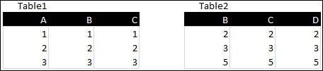
These two tables share two columns, B and C. Then we use the following code to perform a regular join:

Table1:
LOAD * INLINE
[
A, B, C
1, 1, 1
2, 2, 2
3, 3, 3
];
JOIN

LOAD * INLINE
[
B, C, D
2, 2, 2
3, 3, 3
5, 5, 5
];

The result is the following table:

As you can see, the overlapping columns, B and C, have been merged into single columns, and the fields A and D have been added from both tables. It is important to note that, as the second table is being joined to the first the name of the table stays Table1. It is also important to note that the rows that could not be joined, the first and the last, get null values for the missing values.

The JOIN statement can be prefixed with the statements INNER, OUTER, LEFT, and RIGHT, which performs an inner, outer, left, or right join respectively. This has the following results:

Applied to our example tables, the results would be:

The KEEP statement works in the same way that the JOIN statement does, with a small difference. Instead of joining the result in a single table, the KEEP statement keeps both original tables and filters (keeps) rows in one table based on matching rows in another table. The same logic for INNER, OUTER, LEFT, and RIGHT KEEP applies here as did with the JOIN statement.

Let us consider the same two tables from the JOIN example:

If we apply a LEFT KEEP statement to these two tables, like shown in the following code:

Table1:
LOAD * INLINE
[
A, B, C
1, 1, 1
2, 2, 2
3, 3, 3
];

Table2:
LEFT KEEP (Table1)
LOAD * INLINE
[
B, C, D
2, 2, 2
3, 3, 3
5, 5, 5
];

The result we get is the following two tables. As you can see, the last row from the original Table2 has been filtered out as it does not correspond to any of the rows in Table1:

The CONCATENATE statement is also a prefix to the LOAD statement, but instead of matching and merging rows between tables, this statement appends the rows of one table to another table.

Let us again consider the same two tables from the previous example:

We use the following code to concatenate the two tables:

Table1:
LOAD * INLINE
[
A, B, C
1, 1, 1
2, 2, 2
3, 3, 3
];

CONCATENATE (Table1)

LOAD * INLINE
[
B, C, D
2, 2, 2
3, 3, 3
5, 5, 5
];

The result is the following table:

Notice how the rows from the second table were appended to the first table, and that non-matching fields have all been given null values.

When two tables share the exact same columns, QlikView will automatically concatenate them. For example, when looking at the following code we could assume that the result would be two tables, Table1 and Table2.

Table1:
LOAD * INLINE
[
A, B, C
1, 1, 1
2, 2, 2
3, 3, 3
];

Table2:
LOAD * INLINE
[
A, B, C
4, 4, 4
5, 5, 5
6, 6, 6
];

However, in reality, as both tables share the exact same columns, QlikView will implicitly concatenate Table2 onto Table1. The result of this script is a single table.

We can prevent this from happening by prefixing the LOAD statement for Table2 with the NOCONCATENATE statement. This statement instructs QlikView to create a new table, even if a table with the same columns already exists.

The MAPPING statement provides an alternative to the JOIN statement in a very specific scenario: when you want to replace a single key value with a value from a lookup (mapping) table. To see how this works, let's enrich our Aircraft Types dimension table by adding the manufacturer's country. To do this, we open up the script editor and follow these steps:

The modified script for the mapping table should look as follows:

Map_Manufacturer_Country:
MAPPING LOAD Company, 
     Country
FROM
[..Data FilesCSVsAircraft_Manufacturers.csv]
(txt, codepage is 1252, embedded labels, delimiter is ';', msq);

By prefixing the LOAD statement with the MAPPING statement, we tell QlikView that we want to create a mapping table. This is a specific type of table that has the following properties:

We then used the ApplyMap() function to look up the aircraft manufacturer's country while loading the Aircraft_Base_File.csv and Aircraft_2010_Update.csv files. The ApplyMap() function uses three parameters:

Let's look at how this affects the data model:

The COMMENT statement can be used to add comments to tables and fields. These comments will be shown when hovering the mouse cursor over table and field names in various dialogs and the Table Viewer window, and are a very useful aid for understanding the data.

Comments can be added to a table by using the following code:

COMMENT TABLE [Aircraft Types] WITH 'Dimension containing information on aircrafts, including engine types and configuration and manufacturer';

Fields can be commented in the same manner:

COMMENT FIELD [%Aircraft Type ID] WITH 'Primary key of the Aircraft Type dimension';

Of course, commenting each table and field individually in the script is quite a lot of work. Besides that, we often already have our table and field definitions stored outside of QlikView, why would we want to duplicate work? Fortunately, we do not have to. QlikView has the option to use mapping tables for the table and field comments.

Let's open the script editor and apply comments to our Aircraft Types dimension by following these steps:

Our resulting script should look like this:

Map_Table_Comments:
MAPPING LOAD TableName, 
     Comment
FROM
[..Data FilesExcelComments.xls]
(biff, embedded labels, table is Tables$);

Map_Field_Comments:
MAPPING LOAD FieldName,
     Comment
FROM
[..Data FilesExcelComments.xls]
(biff, embedded labels, table is Fields$);

COMMENT TABLES USING Map_Table_Comments;
COMMENT FIELDS USING Map_Field_Comments;

We have now created two mapping tables and have instructed QlikView to use these tables to assign comments to the tables and fields, using the COMMENT TABLES and COMMENT FIELDS statements.

When we save and reload our document and open Table Viewer by pressing Ctrl + T, we should see the comments that we loaded when hovering over the fields of the Aircraft Types table.

Now that we have built our Aircraft Type dimension table, we can use it in our QlikView document. In an environment with multiple documents, it is very likely that we will want to re-use the same table in different apps. Fortunately, there is an easy way to export a QlikView table to an external QVD file; the STORE statement.

We can store the Aircraft Types table to a QVD file by adding the following piece of code at the end of our script:

STORE [Aircraft Types] INTO '..Data FilesQVDsAircraftTypesTransformed.qvd' (qvd);

This tells QlikView to store the table [Aircraft Types] into the sub-folder DataFilesQVDs with the filename AircraftTypesTransformed.qvd The .qvd suffix at the end of the statement tells QlikView to use the QVD format. The other option is (txt) to store the table in text format.

Renaming tables or fields in QlikView is done using the RENAME statement. The following code shows some examples of this statement:

RENAME TABLE [Aircraft Types] TO [Aircraft];
RENAME FIELD [%Aircraft Type ID]  TO [Aircraft ID];
RENAME FIELD [Aircraft Begin Date] to [Begin], [Aircraft End Date] to [End];

As we can see in the third statement, we can also rename multiple fields within the same statement. We can also rename objects by using a mapping table, just like the one we used for the comments. The following code shows an example:

RENAME TABLES USING Map_Table_Names;
RENAME FIELDS USING Map_Field_Names;

Of course, we must not forget to load a mapping table before using this approach.

Deleting tables or fields is done using the DROP statement. The following code shows some examples of dropping table and fields:

DROP TABLE [Aircraft Types];
DROP FIELD [%Aircraft Group Type];
DROP FIELD [%Aircraft Group Type] FROM [Aircraft Types];

The first line deletes the table [Aircraft Types]. The second line deletes the field [%Aircraft Group Type]. The third line also deletes the field [%Aircraft Group Type], but only from the [Aircraft Types] table. If any other tables contain the same field, those are left unaffected.