
At this point in the book, we've already covered topics related to data sources such as extraction, data visualization, scripting, and data modeling. These topics are all interconnected in the development process. We will now complement these four topics with a fifth subject that is of fundamental importance, and one that plays an essential role when developing QlikView apps, taking to an advanced level the lessons learned from all of the previous chapters: Data Transformation.
The topics we'll cover here will help us:
- Make the data sources adequate to meet our data model design requirements
- Deal with unstructured tables (such as Crosstables) and incorporate them into our data model
On we go.
We've seen how the QlikView engine works and the importance of having a data model design that fully takes advantage of QlikView's associative algorithms. So, the first section of this chapter deals with transforming source tables to make them adequate for our data model. The different structure transformations we'll make are:
- "Cleansing" a dirty table
- Converting a Crosstable to a standard table
- Using hierarchy tables
- Loading generic tables
As we've said before, it's not that uncommon for business users to require consolidated information from all sorts of different sources: the CRM, the company's Data Warehouse, Excel tables, Legacy systems, and so on. In these scenarios, the developer commonly faces the challenge of adapting a user file (Excel, CSV, TXT) that has either a non-standard structure or contains "dirty" data which needs to be removed, such as report headers or subtotal lines, and sometimes both.
Fortunately for us, QlikView's data extraction engine is powerful enough to be able to interpret these tables, cleanse them before loading and convert them into a standard table. However, for that to happen, we must specify the set of rules to follow when loading a certain file. These rules and conditions can be set via the Transformation Wizard, available when loading local table files and HTML web files.
To demonstrate how the Transformation Wizard works, we will be using a text file that has been provided along with this book, named Production Planning – Legacy.txt. Look for it inside the Airline OperationsSide ExamplesChapter 10 folder.
The contents of the Production Planning – Legacy.txt file, as seen from a text editor, are shown in the following screenshot:

The structure and contents of the file are described as follows:
- It has a 4-line header, with information about the report above the actual field names.
- Columns in the data area are delimited with tabs.
- Column labels are placed in the fifth line.
- After the column heading there is a "garbage" line intended to be a visual separator.
- The report shows daily data with a weekly subtotal.
- The report shows ten weeks of data, with five of them on the left and the other five placed on the right.
- Records with no specified date correspond to the same date as the previous record.
We have taken the preceding file as an example since it represents a very common way of pulling data out of certain particular systems. Even in popular ERP systems, such as SAP, reports can be generated in this manner. Of course, there may be ways to circumvent the unstructured report and go right to the source table, but in some cases access is a bit restricted.
So, let's start cleaning up this mess.
We will load this file into a new QVW file, so let's begin by creating a new QlikView document and saving it as Production Planning.qvw. This new file will be saved inside the Airline OperationsSide ExamplesChapter 10 folder. After saving the file, make sure the Production Planning – Legacy.txt file is also at the same location.
Next, open the Script Editor (Ctrl+E) and bring up the File Wizard by clicking on the Table Files… button.
Then, browse to the folder in which the text file is stored, select it and click on Open. Right after that, the File Wizard will show the following window:

Make sure the parameters are set as shown in the preceding screenshot so that QlikView interprets the file correctly.
After clicking Next >, the File Wizard: Transform window will appear, showing a brief description about it and a warning:

Essentially, the warning text indicates that the Transformation Step Wizard should not be used for large tables. In our case, the example file contains no more than 50 lines of data, so it won't be a problem for us this time and will rarely be when working with actual "dirty" reports.
Click on the Enable Transformation Step button to access the corresponding features. We will be presented with the following wizard:

As you can see, the Transformation Step Wizard is split into several tabs, and each one is used to handle different scenarios. We will be using three of the five tabs, but will describe what all of them do and the types they could be used.
Our example file certainly has some garbage that needs to be thrown out. We will use the first tab of the Transformation step wizard to:
- Remove the heading rows (first 4 lines)
- Remove the visual separator between the column headings and the actual data
- Remove the weekly totals
Follow these steps to accomplish the above:
- Click on each of the row numbers in the first four lines, as well as in the sixth line, one at a time. The entire row should be highlighted and the Delete Marked button should be enabled, as shown in the following screenshot:

- Click on the Delete Marked button to remove these rows. They should instantly disappear.
- Now, click on the Conditional Delete… button to continue removing the weekly totals. A new window will appear, shown below, in which we will specify the condition on which the remaining rows should be removed.

- Make sure, as in the preceding screenshot, to set the following parameters:
- Click on the Add button to finish setting the condition and then click on OK to return to the previous window.
The preceding procedure will remove the garbage from our file, but that is not all we need to do.
There is another "formatting challenge" we will tackle with this file, which is, that data is split into two parts: the first five weeks are on the left side of the file and weeks 6 - 10 are on the right, occupying the same rows. So, we need to unwrap them.
Essentially, we want to move the data located on the right part of the table and place it below the data located on the left. To do that, we will activate the Unwrap tab from the Transformation Step wizard and follow these steps:
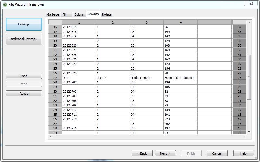
- Use the bar-shaped cursor to mark the beginning of the "right" part of the table by clicking on the column border between columns 4 and 5. This will specify the separation, as seen in the following screenshot. If you don't see where the second part of the table begins, use the scrollbar to move to the right.

- Click Unwrap to move the table content to the appropriate place. We should now see the following result:
The preceding procedure leaves us with a new garbage line: the column headings corresponding to the unwrapped content (shown at line 27 in the preceding screenshot). To remove it, we need to go back to the Garbage tab and follow these steps:
- Click on the Conditional Delete… button to specify the condition on which the rows should be removed.
- From the Specify Row Condition dialog window, we will specify two conditions, joined with an AND operator. For the first condition, mark the following parameters:
- Click on the Add button to include the first condition and then continue setting the second condition with the following parameters:
- Select the Range radio button

- Click on the From button and set the Cell Index Position to 2 From Top. Then, click on OK.

- Now, click on the To button and set the Cell Index Position to 1 From Bottom. Click on OK.

- Click on the Select button and set the Select value to 1 and the Skip value to 0. Click on OK:

- Select the Range radio button
- Click on the Add button to include this second condition and then click on OK.
Now, the two conditions will be evaluated and those rows that match both conditions will be removed.
We had to apply both conditions because if we had only specified the "contains Date" condition the first row would have been removed as well.
Furthermore, if we had deleted line 27 directly by marking it with the mouse and by clicking on the Delete Marked button, even though the effect would have been what we expected, the final code instruction would always look for line 27 and remove it, without first evaluating if that's actually a garbage line. What would happen when the report is updated? Who knows if the garbage line will still be line 27. You can't be sure. It's better to apply a certain logic so that even when you update the report, the code can automatically identify the garbage line.
As we previously said, there are records with no specified date. We will use the Transformation Step Wizard dialog to fill those values. Follow these steps:
- Activate the Fill tab from the Transformation Step Wizard dialog.
- Click on the Fill… button. The following wizard should appear:

- The Target Column field should be 1, as that is where the date values are stored.
- The Fill type will be Above, to take the value that is in the immediate previous record.
- Click on the Cell Condition… button to specify which rows should be filled.

- In the Cell Condition window, make sure the Cell Value field is set to is empty and the Not and Case Sensitive options are disabled. Click on OK twice to return to the Transformation Step window and see the result so far:

As you can see, the missing cells now have the correct date value. Click on the Next > button to exit the Transformation Wizard.
From the File Wizard: Option dialog window, set the Label parameter to Embedded Labels, and then click on Finish to generate the final Load statement.
After specifying the transformation criteria, the corresponding Load statement is automatically generated and, as you will see, all of the settings are specified in the script itself.
The generated script looks as follows:
LOAD Date,
     [Plant #],
     [Product Line ID],
     [Estimated Production]
FROM
[Production Planning - Legacy.txt]
(txt, codepage is 1252, embedded labels, delimiter is '	', msq, filters(
Remove(Row, Pos(Top, 6)),
Remove(Row, Pos(Top, 4)),
Remove(Row, Pos(Top, 3)),
Remove(Row, Pos(Top, 2)),
Remove(Row, Pos(Top, 1)),
Remove(Row, RowCnd(CellValue, 1, StrCnd(contain, 'Total'))),
Unwrap(Col, Pos(Top, 5)),
Remove(Row, RowCnd(Compound,
RowCnd(CellValue, 1, StrCnd(contain, 'Date')),
RowCnd(Interval, Pos(Top, 2), Pos(Bottom, 1), Select(1, 0))
)),
Replace(1, top, StrCnd(null))
));
After reloading the script, we can open the Table Viewer window and see that we have a nicely formatted table with the Production Planning data:

As the code was generated and pasted into the script editor, every time the TXT report is updated we just need to re-run the script to update the data in the QlikView document, without having to go through of all the steps over again.
We've successfully loaded a "dirty" file into QlikView by taking advantage of one of its extraction capabilities. This capability broadens QlikView's ability to consolidate data from disparate sources and empowers the QlikView developer in the data model design process.
Let's look at some other options the Transformation Step Wizard provides:
- Column: This tab allows us to copy data from one column, either in its entirety or based on conditions, and place it into other columns. We can also create new columns based on this copy.
- Rotate: This tab can be used to rotate an entire table to either side or by transposing it.
- Context: This tab is only available when loading HTML files and can be used to extract additional information about the cells, other than what is actually visible (for example, URL links, tags, and so on).
We've uncovered one of the Transformation tools available in QlikView, and now it's time to learn about other functions we can use when extracting data.
To be fair, the example we saw in the preceding section is possible but is actually rare. A more common example of a source table that is unfit for QlikView is the Crosstable.
In this section, we will describe what a Crosstable is for QlikView, why it's not suitable for a data model, and how can we transform it into a traditional table using QlikView's extraction engine.
Let's look at the following input table:
|
Department |
Jan |
Feb |
Mar |
Apr |
May |
Jun |
|---|---|---|---|---|---|---|
|
A |
160 |
336 |
545 |
152 |
437 |
1 |
|
B |
476 |
276 |
560 |
57 |
343 |
476 |
|
C |
251 |
591 |
555 |
195 |
341 |
399 |
|
D |
96 |
423 |
277 |
564 |
590 |
130 |
As you can see, we have one field (column) for each month. We also have a Department field, with its corresponding field values in one single column. The values in the data area of the table are amounts. Let's assume they are Sales amounts.
The problem with this matrix-like structure is that if, for example, we want to obtain the total sales for each department, we would need to create an expression like the following:
Sum (Jan) + Sum(Feb) + Sum(Mar) + Sum(Apr) + Sum(May) + Sum(Jun)
At the same time, we wouldn't be able to create a trend chart, because all months are stored as different dimensions. So, we need to make it fit our purposes.
For us to use this table better in a QlikView data model, we need to convert it to a traditional table with the following structure:
|
Department |
Month |
Sales |
|---|---|---|
|
A |
Jan |
160 |
|
A |
Feb |
336 |
|
A |
Mar |
545 |
|
A |
Apr |
152 |
|
A |
May |
437 |
|
A |
Jun |
1 |
This way, in our charts, we will be able to create expressions such as:
Sum(Sales)
Just as we did with our preceding example, we will load this file into a new QVW, so let's begin by creating a new QlikView document and saving it as Crosstable example.qvw. The new file should be saved in the Airline OperationsSide ExamplesChapter 10 folder.
After saving the file, make sure the Crosstable example.xls file is also at the same location.
Next, open the Script Editor window and bring up the File Wizard by clicking on the Table Files… button.
Browse to the folder in which the example file is stored, select it, and click on Open. Right after that, the file wizard will show the following window:

Make sure the appropriate parameters are set, as shown in the preceding screenshot, so that QlikView interprets the file correctly.
Click on Next > twice and the already familiar File Wizard: Options dialog window opens. Locate the Crosstable… button at the upper-right corner of the window, shown in the following screenshot, and click on it.

The Crosstable wizard only requires us to set three parameters, as shown below:
- Number of Qualifier Fields: Here, we specify the number of columns which precede the table Data Area (where the amounts are). In our case, there is only one Qualifier field:
Department. - Attribute field: This parameter is used to assign a name to the field that will hold the new dimension values resulting from the transformation. For this example, we will , set it to
Month. - Data Field: This indicates the name of the field that will hold the data values resulting from the transformation. We will name it
Sales.
After clicking on OK, the Result tab, at the lower pane of the File Wizard window, will show a preview of the transformed table:

We can now click on Finish and the corresponding Load statement will be generated. The code looks like this:
CrossTable(Month, Sales)
LOAD Department,
     Jan,
     Feb,
     Mar,
     Apr,
     May,
     Jun,
     Jul,
     Aug,
     Sep,
     Oct,
     Nov,
     Dec
FROM
[Crosstable example.xls]
(biff, embedded labels, table is Sheet1$);
Notice there is a prefix to the Load keyword with the names of the new fields. After reloading the script, we will have a table with three fields (Department, Month, and Sales) ready to be used in a QlikView data model.
We've covered the process of loading a Crosstable into QlikView, and now it's your time to put it into practice. We've prepared a table file for you to load into QlikView.
The filename is Employment Statistics – CrossTable.qvd and it is located inside the same Airline OperationsSide ExamplesChapter 10 folder. It contains Airline Employment Data (number of total employees), which the same we used in the previous chapter, but with a Crosstable format.
The challenge for you consists of:
- Identifying the Qualifier fields
- Identifying the name of the Attribute field
- Generating the corresponding Load statement
- Determining how the transformed table can be loaded into the Airline Operations data model
Good luck!
A hierarchy table is a common format to store information in a parent-child structure. The hierarchical nature of the table allows one value to be related to one or more values across the table, as a parent or as a child. In fact, one value can be related to one or more other values as a child and to one or more other different values as a parent.
The advantage of these tables is that they keep the information in a compact format, and QlikView is able to handle them, and expand its relations with a special function: Hierarchy.
Consider the following table which contains hierarchical information about regions of the world:
|
Parent |
Child |
|---|---|
|
World |
Europe |
|
World |
North America |
|
Europe |
England |
|
England |
London |
|
Europe |
Italy |
|
Italy |
Rome |
|
North America |
United States |
|
United States |
Washington |
|
United States |
New York |
The preceding data is the actual format in which the information is stored, but it can also be read as follows, for easier interpretation:

We can see that the shown hierarchy has 4 levels (World – Continent – Country – City). Each of these levels should be stored in a different field in the QlikView data model after expanding the hierarchy.
Again, to demonstrate the concept, we will:
- Create a new QlikView document and name it
Hierarchy example.qvw. - Store the QVW file into the
Airline OperationsSide ExamplesChapter 10folder. - Make sure the
Hierarchy example.xlsfile is also at the same location. - Open the script editor window and bring up the File Wizard dialog with the associated example file.
- In the first window of the File Wizard, make sure the following parameters are set before continuing:

- Then, click on Next > twice to get to the File Wizard: Options dialog window. Locate the Hierarchy… button at the upper-right corner of the window and click on it.
We will then set the parameters in the next window as follows:

The three parameters at the top are mandatory, while the rest are optional.
From the preceding screenshot, we can observe the following fields:
- ID Field: This is the field that stores the IDs corresponding to the child nodes
- Parent ID Field: This is the field that stores the ID of the parent node
- Name field: This is the field that stores the name of the child node
- Parent Name: This is a string used to name a new field that will be created containing the names of the parent nodes
- Path Name: This is a string used to name a new field that will be created containing the list of nodes from the top level to the corresponding node
- Depth Name: This is the name to be assigned to a new field that will hold the number of levels for each expanded node
- Path Source: This is the field from the source table that contains the value that should be used to populate the hierarchy path
- Path Delimiter: This defines the string that should be used to separate the hierarchy values in the path
Even if none of the optional parameters are going to be used, the Hierarchy Parameters checkbox should be marked for the script to be created, otherwise it will not be generated.
Note
We've also noted that, at the time of writing of this book, a bug in QlikView prevents the Depth field (HierarchyLevel in the preceding example) from being populated when using the wizard. Therefore, you may need to manually modify the resulting script in order to create the corresponding field, simply by adding the Depth parameter to the Hierarchy statement, as shown below.
After finishing setting the hierarchy parameters, click on
OK to return to the File Wizard window, and then click on Finish to generate the resulting Load statement.
The resulting script for our example will look like this:
HIERARCHY(Child_ID, Parent_ID, Child, ParentName, Child, Path, ' - ', HierarchyLevel)
LOAD Parent_ID,
     Child_ID,
     Parent,
     Child
FROM
[Hierarchy example.xls]
(biff, embedded labels, table is Sheet1$);
After reloading the script, we should have a new table in our data model with the following structure:

As you can see, the resulting expanded nodes table has one field for each hierarchy level, and one record for each node. Additionally, new fields have been created to show Path and Depth information.
In cases where one node has multiple parents, the expanded nodes table will have several records for these nodes.
Also, it's important to note that the expanded nodes table will exclude any orphan nodes, that is, nodes that have no connection to a top-level node. Only nodes connected to the highest hierarchy level will be kept in the final table.
Once we have a table with this structure, it is easy to use it on the frontend of the QlikView document, for example, within a pivot table or in a hierarchy dimension group.
The created fields can also be used in listboxes to make selections. In fact, let's quickly explore a feature in which we can add a tree-like view to a simple list box.
With the resulting data from the above example, we will create a new list-box object by following these steps:
- Select Layout | New Sheet Object | List Box… from the menu bar.
- From the New List Box window, enter Tree View into the Title field.
- Then, using the Field dropdown, select the
Pathfield. - Still from the General tab, mark the Show as TreeView checkbox and enter a minus sign (
-), with a leading and a trailing space, into the With Separator field. - Click on OK to create the new list box.
The new list box will be created. Here we are taking advantage of the hierarchical path created in one of the fields from the previous exercise. The tree-view list box only requires a field with the hierarchical definition for a set of values, and with each hierarchical level separated by a specific character. The separation symbol can be any character. In the preceding example, we used a minus sign along with a leading and a trailing space since that's how each value is separated in the actual data.
The following screenshot shows a side-by-side comparison of a "normal" list box and the tree-view list box. Both use the same field:

As you can see from the preceding screenshot, a tree-view list box is good at representing hierarchical levels, and provides an easy way to collapse/expand the hierarchy with the plus and minus icons to the left of each parent value.
When clicking a collapsed parent value, all of its children are selected as well.
Another table structure we can come across when loading data into QlikView is what we call a generic table.
A generic table is commonly used to store attribute values for different objects. These attributes are not necessarily shared across all objects contained in the table, and that's one of the reasons why a traditional columnar structure is not used for these tables.
The following is an example of a generic table:
|
Object |
Attribute |
Value |
|---|---|---|
|
Ball |
Color |
Yellow |
|
Ball |
Weight |
120 g |
|
Ball |
Diameter |
8 cm |
|
Coin |
Color |
Gold |
|
Coin |
Value |
$100 |
|
Coin |
Diameter |
2.5 cm |
|
Hockey Puck |
Color |
Black |
|
Hockey Puck |
Diameter |
7.62 cm |
|
Hockey Puck |
Thickness |
2.5 cm |
|
Hockey Puck |
Weight |
165 g |
As you can see, there are several different attributes (color, diameter, weight, and so on) and only a few of them are shared among all objects. Some attributes, such as thickness, are only used for a single object.
Using the preceding structure, the table is kept from growing too large in terms of columns, regardless of new objects or attributes being added.
Using a traditional structure, the preceding table would have several columns (one for each attribute), and each time a new attribute is added, a new column should be added as well. Additionally, attributes (columns) that are not applicable for certain objects (rows), would have a corresponding null or blank value.
When loading a generic table, we can use the GENERIC keyword so QlikView treats the table as such and converts its structure in a way
that is more appropriate for the associative data model and is easier for user interaction.
Let's load this table into a new QlikView document using the GENERIC keyword:
- Start by creating a new QlikView document and name it
Generic Load.qvw. - Store the QVW file into the
Airline OperationsSide ExamplesChapter 10folder. - Make sure the
Generic DB.xlsfile is also at the same location. - Open the script editor and bring up the File Wizard dialog with the associated example file.
- In the first window of the File Wizard, make sure the following parameters are set before continuing:

- Then, click on Finish to close the File Wizard dialog window and generate the corresponding
Loadscript. - Now, right before the
LOADkeyword, enter theGENERICkeyword so that the final script looks as follows:GENERIC LOAD Object, Attribute, Value FROM [Generic DB.xlsx] (ooxml, embedded labels, table is GenericDB);
- Save the document and click on the Reload button from the toolbar.
By using the GENERIC keyword, QlikView will transform and process the contents of the generic table so that, in the end, we have all attributes stored in a separate field and associated to the corresponding object. The resulting data model for the preceding example is shown in the following screenshot:

Each of the tables shown in the preceding screenshot will have only the necessary rows, depending on how many objects share the corresponding attribute.
With the new associated tables, we can add different list boxes to our QlikView document to allow the user to select different attributes and objects.