
i
i
i
i
i
i
i
i
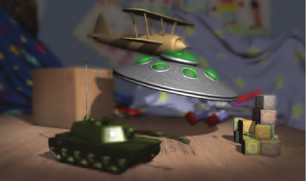
10.13. Depth of Field 489
Figure 10.31. Depth of field using backwards mapping. (Image from “Toy” demo cour-
tesy of NVIDIA Corporation.)
Scattering and gathering techniques both can have problems with oc-
clusion, i.e., one object hiding another. These problems occur at silhouette
edges of objects. A major problem is that objects in the foreground should
have blurred edges. However, only the pixels covered by the foreground
object will be blurred. For example, if a foreground object is in front of
an object in focus, the sample radius will drop to zero when crossing the
silhouette edge on the original image onto the object in focus. This will
cause the foreground object to have an abrupt dropoff, resulting in a sharp
silhouette. Hammon [488] present a scheme that blurs the radius of the
circle of confusion selectively along silhouettes to avoid the sharp dropoff,
while minimizing other artifacts.
A related problem occurs when a sharp silhouette edge from an object in
focus is next to a distant, blurred object. In this case the blurred pixels near
the silhouette edge will gather samples from the object in focus, causing
a halo effect around the silhouette. Scheuermann and Tatarchuk [1121]
use the difference in depths between the pixel and the samples retrieved to
look for this condition. Samples taken that are in focus and are closer than
the pixel’s depth are given lower weights, thereby minimizing this artifact.
Kraus and Strengert [696] present a GPU implementation of a sub-image
blurring technique that avoids many of these edge rendering artifacts.
For further in-depth discussion of depth-of-field algorithms, we refer the
reader to articles by Demers [245], Scheuermann and Tatarchuk [1121], and
Kraus and Strengert [696].
i
i
i
i
i
i
i
i
490 10. Image-Based Effects
10.14 Motion Blur
For interactive applications, to render convincing images it is important
to have both a steady (unvarying) frame rate that is also high enough.
Smooth and continuous motion is preferable, and too low a frame rate is
experienced as jerky motion. Films display at 24 fps, but theaters are dark
and the temporal response of the eye is less sensitive to flicker in the dark.
Also, movie projectors change the image at 24 fps but reduce flickering by
redisplaying each image 2–4 times before displaying the next image. Per-
haps most important, each film frame normally contains a motion-blurred
image; by default, interactive graphics images are not.
In a movie, motion blur comes from the movement of an object across
the screen during a frame. The effect comes from the time a camera’s
shutter is open for 1/40 to 1/60 of a second during the 1/24 of a second
spent on that frame. We are used to seeing this blur in films and consider
it normal, so we expect to also see it in videogames. The hyperkinetic
effect, seen in films such as Gladiator and Saving Private Ryan,iscreated
by having the shutter be open for 1/500 of a second or less.
Rapidly moving objects appear jerky without motion blur, “jumping”
by many pixels between frames. This can be thought of as a type of aliasing,
similar to jaggies, but temporal, rather than spatial in nature. In this sense,
motion blur is a form of temporal antialiasing. Just as increasing display
resolution can reduce jaggies but not eliminate them, increasing frame rate
does not eliminate the need for motion blur. Video games in particular are
characterized by rapid motion of the camera and objects, so motion blur
can significantly improve their visuals. In fact, 30 fps with motion blur
often looks better than 60 fps without [316, 446]. Motion blur can also be
overemphasized for dramatic effect.
Motion blur depends on relative motion. If an object moves from left to
right across the screen, it is blurred horizontally on the screen. If the camera
is tracking a moving object, the object does not blur—the background does.
There are a number of approaches to producing motion blur in computer
rendering. One straightforward, but limited, method is to model and render
the blur itself. This is the rationale for drawing lines to represent moving
particles (see Section 10.7). This concept can be extended.
Imagine a sword slicing through the air. Before and behind the blade,
two polygons are added along its edge. These could be modeled or gener-
ated on the fly by a geometry shader. These polygons use an alpha opacity
per vertex, so that where a polygon meets the sword, it is fully opaque, and
at the outer edge of the polygon, the alpha is fully transparent. The idea is
that the model has transparency to it in the direction of movement, simu-
lating blur. Textures on the object can also be blurred by using techniques
discussed later in this section. Figure 10.32 shows an example.

i
i
i
i
i
i
i
i
10.14. Motion Blur 491
Figure 10.32. Motion blur done by adding geometry to before and behind objects as they
move. Alpha to coverage is used to perform order-independent transparency to avoid
alpha-blending artifacts. (Images from Microsoft SDK [261] sample “MotionBlur10.”)
Figure 10.33. Motion blur done using the accumulation buffer. Note the ghosting on
the arms and legs due to undersampling. Accumulating more images would result in a
smoother blur.
i
i
i
i
i
i
i
i
492 10. Image-Based Effects
The accumulation buffer provides a way to create blur by averaging a
series of images [474]. The object is moved to some set of the positions it
occupies during the frame, and the resulting images are blended together.
The final result gives a blurred image. See Figure 10.33 for an example.
For real-time rendering such a process is normally counterproductive, as it
lowers the frame rate considerably. Also, if objects move rapidly, artifacts
are visible whenever the individual images become discernable. However,
it does converge to a perfectly correct solution, so is useful for creating
reference images for comparison with other techniques.
If what is desired is the suggestion of movement instead of pure realism,
the accumulation buffer concept can be used in a clever way that is not as
costly. Imagine that eight frames of a model in motion have been generated
and stored in an accumulation buffer, then displayed. On the ninth frame,
the model is rendered again and accumulated, but also at this time the first
frame is rendered again and subtracted from the accumulation buffer. The
buffer now has eight frames of a blurred model, frames 2 through 9. On the
next frame, we subtract frame 2 and add in frame 10, giving eight frames,
3 through 10. In this way, only two renderings per frame are needed to
continue to obtain the blur effect [849].
An efficient technique that has seen wide adoption is creation and use
of a velocity buffer [446]. To create this buffer, interpolate the screen-
space velocity at each vertex across the model’s triangles. The velocity
can be computed by having two modeling matrices applied to the model,
one for the last frame and one for the current. The vertex shader pro-
gram computes the difference in positions and transforms this vector to
relative screen-space coordinates. Figure 10.34 shows a velocity buffer and
its results.
Once the velocity buffer is formed, the speed of each object at each pixel
in known. The unblurred image is also rendered. The speed and direction
at a pixel are then used for sampling this image to blur the object. For
example, imagine the velocity of the pixel is left to right (or right to left,
which is equivalent) and that we will take eight samples to compute the
blur. In this case we would take four samples to the left and four to the
right of the pixel, equally spaced. Doing so over the entire object will have
the effect of blurring it horizontally. Such directional blurring is called
line integral convolution (LIC) [148, 534], and it is commonly used for
visualizing fluid flow.
The main problem with using LIC occurs along edges of objects. Sam-
ples should not be taken from areas of the image that are not part of the
object. The interior of the object is correctly blurred, and near the edge
of the object, the background correctly gets blended in. Past the object’s
sharp edge in the velocity buffer there is just the (unmoving) background,
which has no blurring. This transition from blurring to no blurring gives a

i
i
i
i
i
i
i
i
10.14. Motion Blur 493
Figure 10.34. The top image is a visualization of the velocity buffer, showing the screen-
space speed of each object at each pixel, using the red and green channels. The bottom
image shows the effect of blurring using the buffer’s results. (Images from “Killzone 2,”
courtesy of Guerrilla BV.)
sharp, unrealistic discontinuity. A visualization is shown in Figure 10.35.
Some blur near the edges is better than none, but eliminating all disconti-
nuities would be better still.
Green [446] and Shimizu et al. [1167] ameliorate this problem by stretch-
ing the object. Green uses an idea from Wloka to ensure that blurring
happens beyond the boundaries of the object. Wloka’s idea [1364] is to
..................Content has been hidden....................
You can't read the all page of ebook, please click here login for view all page.