

i
i
i
i
i
i
i
i
580 13. Curves and Curved Surfaces
Figure 13.4. Repeated linear interpolation from five points gives a fourth degree (quartic)
B´ezier curve. The curve is inside the conv ex hull (gray region), of the control points,
marked by black dots. Also, at the first point, the curve is tangent to the line between
the first and second poin t. The same also holds for the other end of the curve.
can be described with the recursion formula shown below, where p
0
i
= p
i
are the initial control points:
p
k
i
(t)=(1− t)p
k−1
i
(t)+tp
k−1
i+1
(t),
k =1...n,
i =0...n− k.
(13.3)
Note that a point on the curve is described by p(t)=p
n
0
(t). This is not as
complicated as it looks. Consider again what happens when we construct
aB´ezier curve from three points; p
0
, p
1
,andp
2
, which are equivalent to
p
0
0
, p
0
1
,andp
0
2
. Three controls points means that n =2. Toshortenthe
formulae, sometimes “(t)” is dropped from the p’s. In the fir st step k =1,
which gives p
1
0
=(1− t)p
0
+ tp
1
,andp
1
1
=(1− t)p
1
+ tp
2
. Finally, for
k =2,wegetp
2
0
=(1− t)p
1
0
+ tp
1
1
, which is the same as sought for p(t).
An illustration of how this works in general is shown in Figure 13.5.
Figure 13.5. An illustration of how repeated linear interpolation works for B´ezier curv es.
In this example, the in terpolation of a quartic curve is sho wn. This means there are
five control points, p
0
i
, i =0, 1, 2, 3, 4, shown at the bottom. The diagram should be
read from the bottom up, that is, p
1
0
is formed from weighting p
0
0
with weight 1 − t and
adding that with p
0
1
weighted by t. This goes on until the point of the curve p(t)is
obtained at the top. (Illustration after Goldman [413].)

i
i
i
i
i
i
i
i
13.1. Parametric Cur ves 581
Now that we have the basics in place on how B´ezier curves work, we can
take a look at a more mathematical description of the same curves.
B
´
ezier Curves Using Berns tein Polynomials
As seen in Equation 13.2, the quadratic B´ezier curve could be described
using an algebraic formula. It turns out that every B´ezier curve can be
described with such an algebraic formula, which means that you do not need
to do the repeated interpolation. This is shown below in Equation 13.4,
which yields the same curve as described by Equation 13.3. This description
of the B´ezier curve is called the Bernstein form:
p(t)=
n
i=0
B
n
i
(t)p
i
. (13.4)
This function contains the Bernstein polynomials,
2
B
n
i
(t)=
n
i
t
i
(1 − t)
n−i
=
n!
i!(n − i)!
t
i
(1 − t)
n−i
. (13.5)
The first term, the binomial coefficient, in this equation is defined in Equa-
tion 1.5 in Chapter 1. Two basic properties of the Bernstein polynomial
are the following:
B
n
i
(t) ∈ [0, 1], when t ∈ [0, 1],
n
i=0
B
n
i
(t)=1.
(13.6)
The first formula means that the Bernstein polynomials are in the in-
terval between 0 to 1 when t also is from 0 to 1. The second formula means
that all the Bernstein polynomial terms in Equation 13.4 sum to one for
all different degrees of the curve (this can be seen in Figure 13.6). Loosely
speaking, this means that the curve will stay “close” to the control points,
p
i
. In fact, the entire B´ezier curve will be located in the convex hull (see
Section A.5.3) of the control points, which follows from Equations 13.4
and 13.6. This is a useful property when computing a bounding area or
volume for the curve. See Figure 13.4 for an example.
In Figure 13.6 the Bernstein polynomials for n =1,n =2,andn =3
are shown. These are also called blending functions. The case when n =1
(linear interpolation) is illustrative, in the sense that it shows the curves
y =1− t and y = t. This implies that when t =0,thenp(0) = p
0
,and
when t increases, the blending weight for p
0
decreases, while the blending
weight for p
1
increases by the same amount, keeping the sum of the weights
2
The Bernstein polynomials are sometimes called B´ezier basis functions.

i
i
i
i
i
i
i
i
582 13. Curves and Curved Surfaces
Figure 13.6. Bernstein polynomials for n =1,n =2,andn = 3 (left to right). The
left figure shows linear interpolation, the middle quadratic interpolation, and the right
cubic interpolation. These are the blending functions used in the Bernstein form of
B´ezier curves. So, to evaluate a quadratic curve (middle diagram) at a certain t-value,
just find the t-value on the x-axis, and then go vertically until the three curves are
encountered, which gives the weights for the three control points. Note that B
n
i
(t) ≥ 0,
when t ∈ [0, 1], and the symmetry of these blending functions: B
n
i
(t)=B
n
n−i
(1 − t).
equal to 1. Finally, when t =1,p(1) = p
1
. In general, it holds for
all B´ezier curves that p(0) = p
0
and p(1) = p
n
, that is, the endpoints
are interpolated (i.e., are on the curve). It is also true that the curve is
tangent to the vector p
1
−p
0
at t =0,andtop
n
−p
n−1
at t =1. Another
interesting property is that instead of computing points on a B´ezier curve,
and then rotating the curve, the control points can first be rotated, and
then the points on the curve can be computed. This is a nice property that
most curves and surfaces have, and it means that a program can rotate the
control points (which are few) and then generate the points on the rotated
curve. This is much faster than doing the opposite.
As an example on how the Bernstein version of the B´ezier curve works,
assume that n = 2, i.e., a quadratic curve. Equation 13.4 is then
p(t)=B
2
0
p
0
+ B
2
1
p
1
+ B
2
2
p
2
=
2
0
t
0
(1 − t)
2
p
0
+
2
1
t
1
(1 − t)
1
p
1
+
2
2
t
2
(1 − t)
0
p
2
=(1− t)
2
p
0
+2t(1 − t)p
1
+ t
2
p
2
,
(13.7)
which is the same as Equation 13.2. Note that the blending functions
above, (1 −t)
2
,2t(1 −t), and t
2
, are the functions displayed in the middle
of Figure 13.6. In the same manner, a cubic curve is simplified into the
formula below:
p(t)=(1− t)
3
p
0
+3t(1 − t)
2
p
1
+3t
2
(1 − t)p
2
+ t
3
p
3
. (13.8)
i
i
i
i
i
i
i
i
13.1. Parametric Cur ves 583
This equation can be rewritten in matrix form as
p(t)=
1 tt
2
t
3
⎛
⎜
⎜
⎝
1000
−3300
3 −630
−13−31
⎞
⎟
⎟
⎠
⎛
⎜
⎜
⎝
p
0
p
1
p
2
p
3
⎞
⎟
⎟
⎠
, (13.9)
and since it involves dot products (rather than scalar operations, as in
Equation 13.8), it may be more efficient when implementing on a GPU.
Similarly, Wyatt [1384] argues that B-spline curves can be implemented in
a similar way (just a different matrix), but with many advantages, such as
the natural continuity of that type of curve, among other things. We will
not cover B-splines in this text, other than to say they offer local control.
Any B´ezier curve can be converted to a B-spline, and any B-spline can
be converted to one or more B´ezier curves. Shene’s website [1165] and
Andersson’s article online [22] give easily accessible overviews of B-splines
and other related curves and surfaces. See Further Reading and Resources
at the end of this chapter for more sources of information.
By collecting terms of the form t
k
in Equation 13.4, it can be seen that
every B´ezier curve can be written in the following form, where the c
i
are
points that fall out by collecting terms:
p(t)=
n
i=0
t
i
c
i
. (13.10)
It is straightforward to differentiate Equation 13.4, in order to get the
derivative of the B´ezier curve. The result, after reorganizing and collecting
terms, is shown below [332]:
d
dt
p(t)=n
n−1
i=0
B
n−1
i
(t)(p
i+1
− p
i
). (13.11)
The derivative is, in fact, also a B´ezier curve, but with one degree lower
than p(t).
One downside of B´ezier curves is that they do not pass through all the
control points (except the endpoints). Another problem is that the degree
increases with the number of control points, making evaluation more and
more expensive. A solution to this is to use a simple, low-degree curve
between each pair of subsequent control points, and see to it that this kind
of piecewise interpolation has a high enough degree of continuity. This is
the topic of Sections 13.1.3–13.1.5.
Rational B
´
ezier Cur ves
While B´ezier curves can be used for many things, they do not have that
many degrees of freedom—only the position of the control points can be
i
i
i
i
i
i
i
i
584 13. Curves and Curved Surfaces
chosen freely. Also, not every curve can be described by B´ezier curves.
For example, the circle is normally considered a very simple shape, but it
cannot be described by one or a collection of B´ezier curves. One alternative
is the rational B´ezier curve. This type of curve is described by the formula
shown in Equation 13.12:
p(t)=
n
i=0
w
i
B
n
i
(t)p
i
n
i=0
w
i
B
n
i
(t)
. (13.12)
The denominator is a weighted sum of the Bernstein polynomials, while
the numerator is a weighted version of the standard B´ezier curve (Equa-
tion 13.4). For this type of curve, the user has the weights, w
i
, as additional
degrees of freedom. More about these curves can be found in Hoschek and
Lasser’s [569] and in Farin’s book [332]. Farin also describes how a circle
can be described by three rational B´ezier curves.
13.1.2 Bounded B
´
ezier Curves on the GPU
A method for rendering B´ezier curves on the GPU will be presented [788,
791]. Specifically, the target is “bounded B´ezier curves,” where the region
between the curve and the straight line between the first and last control
points is filled. There is a surprisingly simple way to do this by rendering
a triangle with a specialized pixel shader.
We use a quadratic, i.e., degree two, B´ezier curve, with control points
p
0
, p
1
,andp
2
. See Section 13.1.1. If we set the texture coordinates at
these vertices to t
0
=(0, 0), t
1
=(0.5, 0), and t
2
=(1, 1), the texture
coordinates will be interpolated as usual during rendering of the triangle
Δp
0
p
1
p
2
. We also evaluate the following scalar function inside the triangle
1
0.5
0
0 0.5 1
u
v
v=u
2
f(u,v)<0 f(u,v)>0
t
0
t
1
t
2
p
0
p
1
p
2
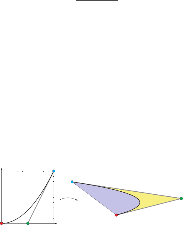
Figure 13.7. Bounded B´ezier curve rendering. Left: The curve is shown in canonical
texture space. Right: The curve is rendered in screenspace. If the condition f(u, v) ≥ 0
is used to kill pixels, then the light blue region will result from the rendering.
..................Content has been hidden....................
You can't read the all page of ebook, please click here login for view all page.