
i
i
i
i
i
i
i
i
16.18. Dynamic Intersection Testing 785
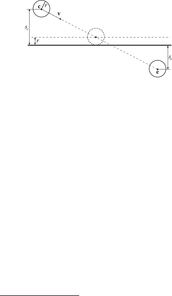
Figure 16.28. The notation used in the dynamic sphere/plane intersection test. The
middle sphere shows the position of the sphere at the time when collision occurs. Note
that s
c
and s
e
are both signed distances.
remaining time to the next frame from the collision, and r is the reflection
vector.
16.18.2 Sphere/Sphere
Testing two moving spheres A and B for intersection turns out to be equiv-
alent to testing a ray against a static sphere—a surprising result. This
equivalency is shown by performing two steps. First, use the principle of
relative motion to make sphere B become static. Then, a technique is bor-
rowed from the frustum/sphere intersection test (Section 16.14.2). In that
test, the sphere was moved along the surface of the frustum to create a
larger frustum. By extending the frustum outwards by the radius of the
sphere, the sphere itself could be shrunk to a point. Here, moving one
sphere over the surface of another sphere results in a new sphere that is
the sum of the radii of the two original spheres.
18
So, the radius of sphere
A is added to the radius of B to give B a new radius. Now we have the
situation where sphere B is static and is larger, and sphere A is a point
moving along a straight line, i.e., a ray. See Figure 16.29.
As this basic intersection test was already presented in Section 16.6, we
will simply present the final result:
(v
AB
· v
AB
)t
2
+2(l · v
AB
)t + l ·l − (r
A
+ r
B
)
2
=0. (16.62)
In this equation, v
AB
= v
A
− v
B
,andl = c
A
− c
B
,wherec
A
and c
B
are the centers of the spheres.
18
This discussion assumes that the spheres do not overlap to start; the intersections
computed by the algorithm here computes where the outsides of the two spheres first
touch.

i
i
i
i
i
i
i
i
786 16. Intersection Test Methods
Figure 16.29. The left figure shows two spheres moving and colliding. In the center
figure, sphere B has been made static by subtracting its velocity from both spheres.
Note that the relative positions of the spheres at the collision point remains the same.
On the right, the radius r
A
of sphere A is added to B and subtracted from itself, making
the moving sphere A into a ray.
This gives a, b,andc:
a =(v
AB
·v
AB
),
b =2(l ·v
AB
),
c = l · l − (r
A
+ r
B
)
2
,
(16.63)
which are values used in the quadratic equation
at
2
+ bt + c =0. (16.64)
The two roots are computed by first computing
q = −
1
2
(b +sign(b)
b
2
− 4ac). (16.65)
Here, sign(b)is+1whenb ≥ 0, else −1. Then the two roots are
t
0
=
q
a
,
t
1
=
c
q
.
(16.66)
This form of solving the quadratic is not what is normally presented in
textbooks, but Press et al. note that it is more numerically stable [1034].
The smallest value in the range [t
0
,t
1
] that lies within [0, 1] (the time
of the frame) is the time of first intersection. Plugging this t-value into
p
A
(t)=c
A
+ tv
A
,
p
B
(t)=c
B
+ tv
B
(16.67)
yields the location of each sphere at the time of first contact. The main
difference of this test and the ray/sphere test presented earlier is that the
ray direction v
AB
is not normalized here.
i
i
i
i
i
i
i
i
16.18. Dynamic Intersection Testing 787
16.18.3 Sphere/Polygon
Dynamic sphere/plane intersection was simple enough to visualize directly.
That said, sphere/plane intersection can be converted to another form in
a similar fashion as done with sphere/sphere intersection. That is, the
moving sphere can be shrunk to a moving point, so forming a ray, and the
plane expanded to a slab the thickness of the sphere’s diameter. The key
idea used in both tests is that of computing what is called the Minkowski
sum of the two objects. The Minkowski sum of a sphere and a sphere is
a larger sphere equal to the radius of both. The sum of a sphere and a
plane is a plane thickened in each direction by the sphere’s radius. Any
two volumes can be added together in this fashion, though sometimes the
result is difficult to describe. For dynamic sphere/polygon testing the idea
is to test a ray against the Minkowski sum of the sphere and polygon.
Intersecting a moving sphere with a polygon is somewhat more involved
than sphere/plane intersection. Schroeder gives a detailed explanation of
this algorithm, and provides code on the web [1137]. We follow his presen-
tation here, making corrections as needed, then show how the Minkowski
sum helps explain why the method works.
If the sphere never overlaps the plane, then no further testing is done.
The sphere/plane test presented previously finds when the sphere first in-
tersects the plane. This intersection pointcanthenbeusedinperforming
a point in polygon test (Section 16.9). If this point is inside the polygon,
the sphere first hits the polygon there and testing is done.
However, this hit point can be outside the polygon but the sphere’s
body can still hit a polygon edge or point while moving further along its
path. If a sphere collides with the infinite line formed by the edge, the first
point of contact p on the sphere will be radius r away from the center:
(c
t
− p) · (c
t
− p)=r
2
, (16.68)
where c
t
= c + tv. The initial position of the sphere is c,anditsveloc-
ity is v. Also, the vector from the sphere’s center to this point will be
perpendicular to the edge:
(c
t
− p) · (p
1
− p
0
)=0. (16.69)
Here, p
0
and p
1
are the vertices of the polygon edge. The hit point’s
location p on the edge’s line is defined by the parametric equation
p = p
0
+ d(p
1
− p
0
), (16.70)
where d is a relative distance from p
0
,andd ∈ [0, 1] for points on the edge.
The variables to compute are the time t of the first intersection with
the edge’s line and the distance d along the edge. The valid intersection

i
i
i
i
i
i
i
i
788 16. Intersection Test Methods
Figure 16.30. Notation for the intersection test of a moving sphere and a polygon edge.
(After Schroeder [1137].)
range for t is [0, 1], i.e., during this frame’s duration. If t is discovered to
be outside this range, the collision does not occur during this frame. The
valid range for d is [0, 1], i.e., the hit point must be on the edge itself, not
beyond the edge’s endpoints. See Figure 16.30.
This set of two equations and two unknowns gives
a = k
ee
k
ss
− k
2
es
,
b =2(k
eg
k
es
− k
ee
k
gs
),
c = k
ee
(k
gg
− r
2
) − k
2
eg
,
(16.71)
where
k
ee
= k
e
·k
e
,k
eg
= k
e
· k
g
,
k
es
= k
e
· k
s
,k
gg
= k
g
· k
g
,
k
gs
= k
g
· k
s
,k
ss
= k
s
· k
s
,
(16.72)
and
k
e
= p
1
− p
0
,
k
g
= p
0
− c,
k
s
= e − c = v.
(16.73)
Note that k
s
= v, the velocity vector for one frame, since e is the
destination point for the sphere. This gives a, b,andc, which are the
variables of the quadratic equation in Equation 16.64 on page 786, and so
solved for t
0
and t
1
in the same fashion.
This test is done for each edge of the polygon, and if the range [t
0
,t
1
]
overlaps the range [0, 1], then the edge’s line is intersected by the sphere
in this frame at the smallest value in the intersection of these ranges. The
sphere’s center c
t
at first intersection time t is computed and yields a
distance
d =
(c
t
− p
0
) · k
e
k
ee
, (16.74)
i
i
i
i
i
i
i
i
16.18. Dynamic Intersection Testing 789
whichneedstobeintherange[0, 1]. If d is not in this range, the edge is
considered missed.
19
Using this d in Equation 16.70 gives the point where
the sphere first intersects the edge. Note that if the point of first intersec-
tion is needed, then all three edges must be tested against the sphere, as
the sphere could hit more than one edge.
The sphere/edge test is computationally complex. One optimization for
this test is to put an AABB around the sphere’s path for the frame and
test the edge as a ray against this box before doing this full test. If the
line segment does not overlap the AABB, then the edge cannot intersect
the sphere [1137].
If no edge is the first point of intersection for the sphere, further testing
is needed. Recall that the sphere is being tested against the first point of
contact with the polygon. A sphere may eventually hit the interior or an
edge of a polygon, but the tests given here check only for first intersection.
The third possibility is that the first point of contact is a polygon vertex.
So, each vertex in turn is tested against the sphere. Using the concept of
relative motion, testing a moving sphere against a static point is exactly
equivalent to testing a sphere against a moving point, i.e., a ray. Using the
ray/sphere intersection routine in Section 16.6 is then all that is needed.
To test the ray c
t
= c + tv against a sphere centered at p
0
with radius,
r, results can be reused from the previous edge computations to solve t,as
follows:
a = k
ss
,
b = −2k
gs
,
c = k
gg
− r
2
.
(16.75)
Using this form avoids having to normalize the ray direction for
ray/sphere intersection. As before, solve the quadratic equation shown
in Equation 16.64 and use the lowest valid root to compute when in the
frame the sphere first intersects the vertex. The point of intersection is the
vertex itself, of course.
In truth, this sphere/polygon test is equivalent to testing a ray (rep-
resented by the center of the sphere moving along a line) against the
Minkowski sum of the sphere and polygon. This summed surface is one
in which the vertices have been turned into spheres of radius r,theedges
into cylinders of radius r, and the polygon itself raised and lowered by r
to seal off the object. See Figure 16.31 for a visualization of this. This is
the same sort of expansion as done for frustum/sphere intersection (Sec-
tion 16.14.2). So the algorithm presented can be thought of as testing a
19
In fact, the edge could be hit by the sphere, but the hit point computed here would
not be where contact is actually made. The sphere will first hit one of the vertex
endpoints, and this test follows next.
..................Content has been hidden....................
You can't read the all page of ebook, please click here login for view all page.