

i
i
i
i
i
i
i
i
392 9. Global Illumination
Figure 9.46. Recursive reflections, done with environment mapping. (Image courtesy of
Kasper Høy Nielsen.)
Other extensions of the environment mapping technique can enable
more general reflections. Hakura et al. [490] show how a set of EMs can
be used to capture local interreflections, i.e., when a part of an object is
reflected in itself. Such methods are very expensive in terms of texture
memory. Rendering a teapot with ray tracing quality required 100 EMs
of 256 × 256 resolution. Umenhoffer et al. [1282] describe an extension of
environment mapping in which a few of the closest layers of the scene are
stored along with their depths and normals per pixel. The idea is like depth
peeling, but for forming layers of successive environment maps, which they
call layered distance maps. This allows objects hidden from view from the
center point of the EM to be revealed when reflection rays originate from
a different location on the reflector’s surface. Accurate multiple reflections
and self-reflections are possible. This algorithm is interesting in that it lies
in a space between environment mapping, image-based rendering, and ray
tracing.
9.4 Transmittance
As discussed in Section 5.7, a transparent surface can be treated as a blend
color or a filter color. When blending, the transmitter’s color is mixed with
the incoming color from the objects seen through the transmitter. The

i
i
i
i
i
i
i
i
9.4. Transmittance 393
over operator uses the α value as an opacity to blend these two colors.
The transmitter color is multiplied by α, the incoming color by 1 −α,and
the two summed. So, for example, a higher opacity means more of the
transmitter’s color and less of the incoming color affects the pixel. While
this gives a visual sense of transparency to a surface [554], it has little
physical basis.
Multiplying the incoming color by a transmitter’s filter color is more
in keeping with how the physical world works. Say a blue-tinted filter is
attached to a camera lens. The filter absorbs or reflects light in such a
way that its spectrum resolves to a blue color. The exact spectrum is
usually unimportant, so using the RGB equivalent color works fairly well
in practice. For a thin object like a filter, stained glass, windows, etc., we
simply ignore the thickness and assign a filter color.
For objects that vary in thickness, the amount of light absorption can
be computed using the Beer-Lambert Law:
T = e
−α
cd
, (9.26)
where T is the transmittance, α
is the absorption coefficient, c is the
concentration of the absorbing material, and d is the distance traveled
through the glass, i.e., the thickness. The key idea is that the transmitting
medium, e.g., the glass, absorbs light relative to e
−d
. While α
and c are
physical values, to make a transmittance filter easy to control, Bavoil [74]
sets the value c to be the least amount of transmittance at some given
thickness, defined to be a maximum concentration of 1.0. These settings
give
T = e
−α
d
user
, (9.27)
so
α
=
−log(T )
d
user
. (9.28)
Note that a transmittance of 0 needs to be handled as a special case. A
simple solution is to add some small epsilon, e.g., 0.000001, to each T .The
effect of color filtering is shown in Figure 9.47.
E
XAMPLE:TRANSMIT TANCE. The user decides the darkest transmittance
filter color should be (0.3,0.7,0.1) for a thickness of 4.0 inches (the unit
type does not matter, as long as it is consistent). The α
values for these
RGB channels are:
α
r
=
− log(0.3)
4.0
=0.3010,
α
g
=
− log(0.7)
4.0
=0.0892,
α
b
=
− log(0.1)
4.0
=0.5756.
(9.29)

i
i
i
i
i
i
i
i
394 9. Global Illumination
Figure 9.47. Translucency with different absorption factors. (Images courtesy of Louis
Bavoil.)
In creating the material, the artist sets the concentration down to 0.6,
letting more light through. During shading, thickness of the transmitter is
found to be 1.32 for a fragment. The transmitter filter color is then:
T
r
= e
−0.3010×0.6×1.32
=0.7879,
T
g
= e
−0.0892×0.6×1.32
=0.9318,
T
b
= e
−0.5756×0.6×1.32
=0.6339.
(9.30)
The color stored in the underlying pixel is then multiplied by this color
(0.7879, 0.9318, 0.6339), to get the resulting transmitted color.
Varying the transmittance by distance traveled can work as a reason-
able approximation for other phenomena. For example, Figure 10.40 on
page 500 shows layered fog using the fog’s thickness. In this case, the
incoming light is attenuated by absorption and by out-scattering, where
light bounces off the water particles in the fog in a different direction. In-
scattering, where light from elsewhere in the environment bounces off the
particles toward the eye, is used to represent the white fog.
Computing the actual thickness of the transmitting medium can be
done in any number of ways. A common, general method to use is to first
render the surface where the view ray exits the transmitter. This surface
could be the backface of a crystal ball, or could be the sea floor (i.e., where
the water ends). The z-depth or location of this surface is stored. Then
the transmitter’s surface is rendered. In a shader program, the stored z-
depth is accessed and the distance between it and the transmitter’s surface
location is computed. This distance is then used to compute the amount
of transmittance for the incoming light, i.e., for the object behind the
transmitter.
This method works if it is guaranteed that the transmitter has one entry
and one exit point per pixel, as with a crystal ball or seabed. For more elab-
i
i
i
i
i
i
i
i
9.4. Transmittance 395
orate models, e.g., a glass sculpture or other object with concavities, two
or more separate spans may absorb incoming light. Using depth peeling, as
discussed in Section 5.7, we can render the transmitter surfaces in precise
back-to-front order. As each frontface is rendered, the distance through
the transmitter is computed and used to compute absorption. Applying
each of these in turn gives the proper final transmittance. Note that if all
transmitters are made of the same material at the same concentration, the
shade could be computed once at the end using the summed distances, if
the surface has no reflective component. See Section 10.15 about fog for
related techniques.
Most transmitting media have an index of refraction significantly higher
than that of air. This will cause light to undergo external reflection when
entering the medium, and internal reflection when exiting it. Of the two,
internal reflection will attenuate light more strongly. At glancing angles, all
the light will bounce back from the interface, and none will be transmitted
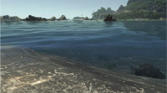
(total internal reflection). Figure 9.48 shows this effect; objects underwater
are visible when looking directly into the water, but looking farther out,
at a grazing angle, the water’s surface mostly hides what is beneath the
waves. There are a number of articles on handling reflection, absorption,
and refraction for large bodies of water [174, 608, 729]. Section 7.5.3 details
how reflectance and transmittance vary with material and angle.
Figure 9.48. Water, taking into account the Fresnel effect, where reflectivity increases
as the angle to the transmitter’s surface becomes shallow. Looking down, reflectivity
is low and we can see into the water. Near the horizon the water becomes much more
reflective. (Image from “Crysis” courtesy of Crytek.)
i
i
i
i
i
i
i
i
396 9. Global Illumination
9.5 Refractions
For simple transmittance, we assume that the incoming light comes from
directly beyond the transmitter. This is a reasonable assumption when the
front and back surfaces of the transmitter are parallel and the thickness
is not great, e.g., for a pane of glass. For other transparent media, the
index of refraction plays an important part. Snell’s Law, which describes
how light changes direction when a transmitter’s surface is encountered, is
described in Section 7.5.3.
Bec [78] presents an efficient method of computing the refraction vector.
For readability (because n is traditionally used for the index of refraction
in Snell’s equation), define N as the surface normal and L as the direction
to the light:
t =(w − k)N − nL, (9.31)
where n = n
1
/n
2
is the relative index of refraction, and
w = n(L · N),
k =
1+(w −n)(w + n).
(9.32)
The resulting refraction vector t is returned normalized.
This evaluation can nonetheless be expensive. Oliveira [962] notes that
because the contribution of refraction drops off near the horizon, an ap-
proximation for incoming angles near the normal direction is
t = −cN − L, (9.33)
where c is somewhere around 1.0 for simulating water. Note that the
resulting vector t needs to be normalized when using this formula.
The index of refraction varies with wavelength. That is, a transpar-
ent medium will bend different colors of light at different angles. This
phenomenon is called dispersion, and explains why prisms work and why
rainbows occur. Dispersion can cause a problem in lenses, called chromatic
aberration. In photography, this phenomenon is called purple fringing,and
can be particularly noticeable along high contrast edges in daylight. In
computer graphics we normally ignore this effect, as it is usually an arti-
fact to be avoided. Additional computation is needed to properly simulate
the effect, as each light ray entering a transparent surface generates a set
of light rays that must then be tracked. As such, normally a single re-
fracted ray is used. In practical terms, water has an index of refraction of
approximately 1.33, glass typically around 1.5, and air essentially 1.0.
Some techniques for simulating refraction are somewhat comparable to
those of reflection. However, for refraction through a planar surface, it is
not as straightforward as just moving the viewpoint. Diefenbach [252] dis-
cusses this problem in depth, noting that a homogeneous transform matrix
..................Content has been hidden....................
You can't read the all page of ebook, please click here login for view all page.