
i
i
i
i
i
i
i
i
Chapter 16
Intersection Test Methods
“I’ll sit and see if that small sailing cloud
Will hit or miss the moon.”
—Robert Frost
Intersection testing is often used in computer graphics. We may wish to
click the mouse on an object, or to determine whether two objects collide,
or to make sure we maintain a constant height off the floor for our viewer
as we navigate a building. All of these operations can be performed with
intersection tests. In this chapter, we cover the most common ray/object
and object/object intersection tests.
In interactive computer graphics applications, it is often desirable to
let the user select a certain object by picking (clicking) on it with the
mouse or any other input device. Naturally, the performance of such an
operation needs to be high. One picking method, supported by OpenGL, is
to render all objects into a tiny pick window. All the objects that overlap
the window are returned in a list, along with the minimum and maximum
z-depth found for each object. This sort of system usually has the added
advantage of being able to pick on lines and vertices in addition to surfaces.
This pick method is always implemented entirely on the host processor and
does not use the graphics accelerator. Some other picking methods do use
the graphics hardware, and are covered in Section 16.1.
Intersection testing offers some benefits that OpenGL’s picking method
does not. Comparing a ray against a triangle is normally faster than send-
ing the triangle through OpenGL, having it clipped against a pick window,
then inquiring whether the triangle was picked. Intersection testing meth-
ods can compute the location, normal vector, texture coordinates, and
other surface data. Such methods are also independent of API support (or
lack thereof).
The picking problem can be solved efficiently by using a bounding vol-
ume hierarchy (see Section 14.1.1). First, we compute the ray from the
camera’s position through the pixel that the user picked. Then, we recur-
sively test whether this ray hits a bounding volume of the hierarchy. If at
725
i
i
i
i
i
i
i
i
726 16. Intersection Test Methods
any time the ray misses a bounding volume (BV), then that subtree can be
discarded from further tests, since the ray will not hit any of its contents.
However, if the ray hits a BV, its children’s BVs must be tested as well.
Finally, the recursion may end in a leaf that contains geometry, in which
case the ray must be tested against each primitive in the geometry node.
As we have seen in Section 14.3, view frustum culling is a means for
efficiently discarding geometry that is outside the view frustum. Tests
that decide whether a bounding volume is totally outside, totally inside, or
partially inside a frustum are needed to use this method.
In collision detection algorithms (see Chapter 17), which are also built
upon hierarchies, the system must decide whether or not two primitive
objects collide. These primitive objects include triangles, spheres, axis-
aligned bounding boxes (AABBs), oriented bounding boxes (OBBs), and
discrete oriented polytopes (k-DOPs).
In all of these cases, we have encountered a certain class of problems
that require intersection tests. An intersection test determines whether two
objects, A and B, intersect, which may mean that A is totally inside B
(or vice versa), that the boundaries of A and B intersect, or that they are
totally disjoint. However, sometimes more information may be needed, such
as the closest intersection point, the distance to this intersection point, etc.
In this chapter, a set of fast intersection test methods is identified and
studied thoroughly. We not only present the basic algorithms, but also
give advice on how to construct new and efficient intersection test meth-
ods. Naturally, the methods presented in this chapter are also of use in
offline computer graphics applications. For example, the algorithms pre-
sented in Sections 16.6 through 16.9 can be used in ray tracing and global
illumination programs.
After briefly covering hardware-accelerated picking methods, this chap-
ter continues with some useful definitions, followed by algorithms for form-
ing bounding volumes around primitives. Rules of thumb for constructing
efficient intersection test methods are presented next. Finally, the bulk of
the chapter is made up of a cookbook of intersection test methods.
16.1 Hardware-Accelerated Picking
There are a few hardware-accelerated picking methods worth mentioning.
One method was first presented by Hanrahan and Haeberli [497]. To sup-
port picking, the scene is rendered with each polygon having a unique color
value that is used as an identifier. The image formed is stored offscreen and
is then used for extremely rapid picking. When the user clicks on a pixel,
the color identifier is looked up in this image and the polygon is immedi-
ately identified. The major disadvantage of this method is that the entire
i
i
i
i
i
i
i
i
16.2. Definitions and Tools 727
scene must be rendered in a separate pass to support this sort of picking.
This method was originally presented in the context of a three-dimensional
paint system. In this sort of application, the amount of picking per view is
extremely high, so the cost of forming the buffer once for the view becomes
inconsequential.
It is also possible to find the relative location of a point inside a trian-
gle using the color buffer [724]. Each triangle is rendered using Gouraud
shading, where the colors of the triangle vertices are red (255, 0, 0), green
(0, 255, 0), and blue (0, 0, 255). Say that the color of the picked pixel is
(23, 192, 40), This means that the red vertex contributes with a factor
23/255, the green with 192/255, and the red with 40/255. This information
can be used to find out the actual coordinates on the triangle, the (u, v)co-
ordinates of the picked point, and for normal interpolation. The values are
barycentric coordinates, which are discussed further in Section 16.8.1. In
the same manner, the normals of the vertices can be directly encoded into
RGB colors. The interval [−1, 1] per normal component has to be trans-
formed to the interval [0, 1] so it can be rendered. Alternatively, rendering
can be done directly to a floating-point buffer without the transform. Af-
ter rendering the triangles using Gouraud shading, the normal at any point
can be read from the color buffer.
The possibilities for using the GPU to accelerate selection directly in-
crease considerably with newer hardware and APIs. Features such as the
geometry shader, stream out, and triangle identifiers being available to
shader programs open up new ways to generate selection sets and know
what is in a pick window.
16.2 Definitions and Tools
This section introduces notation and definitions useful for this entire
chapter.
Aray,r(t), is defined by an origin point, o, and a direction vector, d
(which, for convenience, is usually normalized, so ||d|| =1). Itsmathe-
matical formula is shown in Equation 16.1, and an illustration of a ray is
shown in Figure 16.1:
r(t)=o + td. (16.1)
The scalar t is a variable that is used to generate different points on the
ray, where t-values of less than zero are said to lie behind the ray origin
(and so are not part of the ray), and the positive t-values lie in front of it.
Also, since the ray direction is normalized, a t-value generates a point on
the ray that is situated t distance units from the ray origin.

i
i
i
i
i
i
i
i
728 16. Intersection Test Methods
Figure 16.1. A simple ray and its parameters: o (the ray origin), d (the ray direction),
and t, which generates different points on the ray, r(t)=o + td.
In practice, we often also store a current distance l, which is the maxi-
mum distance we want to search along the ray. For example, while picking,
we usually want the closest intersection along the ray; objects beyond this
intersection can be safely ignored. The distance l starts at ∞. As objects
are successfully intersected, l is updated with the intersection distance. In
the ray/object intersection tests we will be discussing, we will normally
not include l in the discussion. If you wish to use l,allyouhavetodois
perform the ordinary ray/object test, then check l against the intersection
distance computed and take the appropriate action.
When talking about surfaces, we distinguish implicit surfaces from ex-
plicit surfaces. An implicit surface is defined by Equation 16.2:
f(p)=f(p
x
,p
y
,p
z
)=0. (16.2)
Here, p is any point on the surface. This means that if you have a point
that lies on the surface and you plug this point into f, then the result will
be 0. Otherwise, the result from f will be nonzero. An example of an
implicit surface is p
2
x
+ p
2
y
+ p
2
z
= r
2
, which describes a sphere located
at the origin with radius r. It is easily seen that this can be rewritten
as f (p)=p
2
x
+ p
2
y
+ p
2
z
− r
2
= 0, which means that it is indeed implicit.
Implicit surfaces are briefly covered in Section 13.3, while modeling and
rendering with a wide variety of implicit surface types is well covered in
Bloomenthal et al. [117].
An explicit surface, on the other hand, is defined by a vector function
f and some parameters (ρ, φ), rather than a point on the surface. These
parameters yield points, p, on the surface. Equation 16.3 below shows the
general idea:
p =
⎛
⎝
p
x
p
y
p
z
⎞
⎠
= f(ρ, φ)=
⎛
⎝
f
x
(ρ, φ)
f
y
(ρ, φ)
f
z
(ρ, φ)
⎞
⎠
. (16.3)
An example of an explicit surface is again the sphere, this time expressed
in spherical coordinates, where ρ is the latitude and φ longitude, as shown
i
i
i
i
i
i
i
i
16.2. Definitions and Tools 729
x
y
z
a
min
a
max
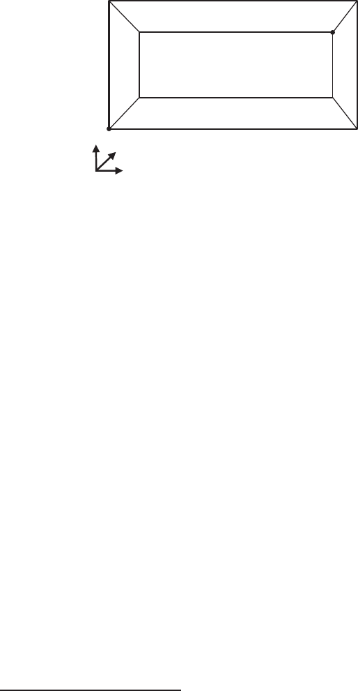
Figure 16.2. A three-dimensional AABB, A, with its extreme points, a
min
and a
max
,
and the axes of the standard basis.
in Equation 16.4:
f(ρ, φ)=
⎛
⎝
r sin ρ cos φ
r sin ρ sin φ
r cos ρ
⎞
⎠
(16.4)
As another example, a triangle, v
0
v
1
v
2
, can be described in explicit form
like this: t(u, v)=(1− u − v)v
0
+ uv
1
+ vv
2
,whereu ≥ 0, v ≥ 0and
u + v ≤ 1 must hold.
Finally, we shall give definitions of three bounding volumes, namely the
AABB, the OBB, and the k-DOP, used extensively in this and the next
chapter.
Definition. An axis-aligned bounding box
1
(also called a rectangular box),
AABB for short, is a box whose faces have normals that coincide with the
standard basis axes. For example, an AABB A is described by two diago-
nally opposite points, a
min
and a
max
,wherea
min
i
≤ a
max
i
, ∀i ∈{x, y, z}.
Figure 16.2 contains an illustration of a three-dimensional AABB to-
gether with notation.
Definition. An oriented bounding box, OBB for short, is a box whose faces
have normals that are all pairwise orthogonal—i.e., it is an AABB that is
arbitrarily rotated. An OBB, B, can be described by the center point of
the box, b
c
, and three normalized vectors, b
u
, b
v
,andb
w
, that describe
the side directions of the box. Their respective positive half-lengths are
denoted h
B
u
, h
B
v
,andh
B
w
, which is the distance from b
c
to the center of the
respective face.
1
In fact, neither the AABB nor OBB needs to be used as a BV, but can act as a pure
geometric box. However, these names are widely accepted.
..................Content has been hidden....................
You can't read the all page of ebook, please click here login for view all page.