

i
i
i
i
i
i
i
i
14.1. Spatial Data Structures 655
Figure 14.5. The construction of a quadtree. The construction starts from the left by
enclosing all objects in a bounding box. Then the boxes are recursively divided into four
equal-sized boxes until each box (in this case) is empty or contains one object.
Octrees can be used in the same manner as axis-aligned BSP trees, and
thus, can handle the same types of queries. They are also used in occlu-
sion culling algorithms (see Section 14.6.2). A BSP tree can, in fact, give
the same partitioning of space as an octree. If a cell is first split along
themiddleof,say,theX-axis, then the two children are split along the
middle of, say, Y , and finally those children are split in the middle along
Z, eight equal-sized cells are formed that are the same as those created
by one application of an octree division. One source of efficiency for the
octree is that it does not need to store information needed by more flex-
ible BSP tree structures. For example, the splitting plane locations are
known and so do not have to be described explicitly. This more compact
storage scheme also saves time by accessing fewer memory locations dur-
ing traversal. Axis-aligned BSP trees can still be more efficient, as the
additional memory cost and traversal time due to the need for retrieving
the splitting plane’s location can be outweighed by the savings from better
plane placement. There is no overall best efficiency scheme; it depends on
the nature of the underlying geometry, the use pattern of how the struc-
ture is accessed, and the architecture of the hardware running the code, to
name a few factors. Often the locality and level of cache-friendliness of the
memory layout is the most important factor. This is the focus of the next
section.
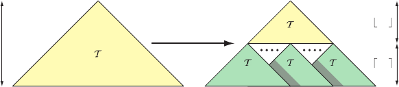
In the above description, objects are always stored in leaf nodes; there-
fore, certain objects have to be stored in more than one leaf node. Another
option is to place the object in the box that is the smallest that contains
the entire object. For example, the star-shaped object in the figure should
be placed in the upper right box in the second illustration from the left.
This has a significant disadvantage in that, for example, a (small) object
that is located at the center of the octree will be placed in the topmost
(largest) node. This is not efficient, since a tiny object is then bounded by
the box that encloses the entire scene. One solution is to split the objects,

i
i
i
i
i
i
i
i
656 14. Acceleration Algorithms
Figure 14.6. An ordinary octree compared to a loose octree. The dots indicate the center
points of the boxes (in the first subdivision). To the left, the star pierces through one
splitting plane of the ordinary octree. Thus, one choice is to put the star in the largest
box (that of the root). To the right, a loose octree with k =1.5 (that is, boxes are 50%
larger) is shown. The boxes are slightly displaced, so that they can be discerned. The
star can now be placed fully in the upper left box.
but that introduces more primitives. Another is to put a pointer to the
object in each leaf box it is in, losing efficiency and making octree editing
more difficult.
Ulrich presents a third solution, loose octrees [1279]. The basic idea of
loose octrees is the same as for ordinary octrees, but the choice of the size
of each box is relaxed. If the side length of an ordinary box is l,thenkl is
used instead, where k>1. This is illustrated for k =1.5, and compared
to an ordinary octree, in Figure 14.6. Note that the boxes’ center points
are the same. By using larger boxes, the number of objects that cross a
splitting plane is reduced, so that the object can be placed deeper down
in the octree. An object is always inserted into only one octree node, so
deletion from the octree is trivial. Some advantages accrue by using k =2.
First, insertion and deletion of objects is O(1). Knowing the object’s size
means immediately knowing the level of the octree it can successfully be
inserted in, fully fitting into one loose box.
2
The object’s centroid deter-
mines into which loose octree box it is put. Because of these properties,
this structure lends itself well to bounding dynamic objects, at the expense
of some BV efficiency, and the loss of a strong sort order when travers-
ing the structure. Also, often an object moves only slightly from frame
to frame, so that the previous box still is valid in the next frame. There-
fore, only a fraction of animated objects in the octree need updating each
frame.
2
In practice it is sometimes possible to push the object to a deeper box in the octree.
Also, if k<2, the object may have to be pushed up the tree if it does not fit.
i
i
i
i
i
i
i
i
14.1. Spatial Data Structures 657
14.1.4 Cache-Oblivious and Cache-Aware
Representations
Since the gap between the bandwidth of the memory system and the com-
puting power of CPUs increases every year, it is very important to de-
sign algorithms and spatial data structure representations with caching in
mind. In this section, we will give an introduction to cache-aware (or cache-
conscious) and cache-oblivious spatial data structures. A cache-aware rep-
resentation assumes that the size of cache blocks is known, and hence we
optimize for a particular architecture. In contrast, a cache-oblivious algo-
rithm is designed to work well for all types of cache sizes, and are hence
platform-independent.
To create a cache-aware data structure, you must first find out what
the size of a cache block is for your architecture. This may be 64 bytes,
for example. Then try to minimize the size of your data structure. For
example, Ericson [315] shows how it is sufficient to use only 32 bits for a k-
d tree node. This is done in part by appropriating the two least significant
bits of the node’s 32-bit value. These two bits can represent four types: a
leaf node, or the internal node split on one of the three axes. For leaf nodes,
the upper 30 bits hold a pointer to a list of objects; for internal nodes, these
represent a (slightly lower precision) floating point split value. Hence, it
is possible to store a four-level deep binary tree of 15 nodes in a single
cache block of 64 bytes (the sixteenth node indicates which children exist
and where they are located). See his book for details. The key concept is
that data access is considerably improved by ensuring that structures pack
cleanly to cache boundaries.
One popular and simple cache-oblivious ordering for trees is the van
Emde Boas layout [32, 315, 1296]. Assume we have a tree, T ,withheight
h. The goal is to compute a cache-oblivious layout, or ordering, of the
nodes in the tree. Let us denote the van Emde Boas layout of T as v(T ).
This structure is defined recursively, and the layout of a single node in a
tree is just the node itself. If there are more than one node in T ,thetreeis
split at half the height, h/2. The topmost h/2 levels are put in a tree
denoted T
0
, and the children subtree starting at the leaf nodes of T
0
are
denoted T
1
,...,T
n
. The recursive nature of the tree is described as follows:
v(T )=
{T } , if there is single node in T ,
{T
0
, T
1
,...,T
n
} ,else.
(14.2)
Note that all of the subtrees T
i
,0≤ i ≤ n, are also defined by the recursion
above. This means, for example, that T
1
has to be split at half its height,
and so on. See Figure 14.7 for an example.
In general, creating a cache-oblivious layout consists of two steps: clus-
tering and ordering of the clusters. For the van Emde Boas layout, the
i
i
i
i
i
i
i
i
658 14. Acceleration Algorithms
0
0
1
1
k
k
n
n
h
h/2
h/2
Figure 14.7. The van Emde Boas layout of a tree, T , is created by splitting the height,
h, of the tree in two. This creates the subtrees, T
0
, T
1
,...,T
n
, and each subtree is split
recursively in the same manner until only one node per subtree remains.
clustering is given by the subtrees, and the ordering is implicit in the cre-
ation order. Yoon et al. [1395, 1396] develop techniques that are specifically
designed for efficient bounding volume hierarchies and BSP trees. They
develop a probabilistic model that takes into account both the locality be-
tween a parent and its children, and the spatial locality. The idea is to
minimize cache misses when a parent has been accessed, by making sure
that the children are inexpensive to access. Furthermore, nodes that are
close to each other are grouped closer together in the ordering. A greedy
algorithm is developed that clusters nodes with the highest probabilities.
Generous increases in performance are obtained without altering the un-
derlying algorithm—it is only the ordering of the nodes in the BVH that
is different.
14.1.5 Scene Graphs
BVHs, BSP trees, and octrees all use some sort of tree as their basic data
structure; it is in how they partition the space and store the geometry
that they differ. They also store geometrical objects, and nothing else, in a
hierarchical fashion. However, rendering a three-dimensional scene is about
so much more than just geometry. Control of animation, visibility, and
other elements are usually performed using a scene graph. Thisisauser-
oriented tree structure that is augmented with textures, transforms, levels
of detail, render states (material properties, for example), light sources, and
whatever else is found suitable. It is represented by a tree, and this tree
is traversed in depth-first order to render the scene. For example, a light
source can be put at an internal node, which affects only the contents of
its subtree. Another example is when a material is encountered in the tree.
The material can be applied to all the geometry in that node’s subtree,
or possibly be overridden by a child’s settings. See also Figure 14.26 on
page 688 on how different levels of detail can be supported in a scene
graph. In a sense, every graphics application uses some form of scene
graph, even if the graph is just a root node with a list of children to
display.

i
i
i
i
i
i
i
i
14.1. Spatial Data Structures 659
Figure 14.8. A scene graph with different transforms M and N applied to internal nodes,
and their respective subtrees. Note that these two internal nodes also point to the same
object, but since they have different transforms, two different objects appear (one is
rotated and scaled).
One way of animating objects is to vary transforms in internal nodes in
the tree. Scene graph implementations then transform the entire contents
of that node’s subtree. Since a transform can be put in any internal node,
hierarchical animation can be done. For example, the wheels of a car can
spin, and the car as a whole can move forward.
When several nodes may point to the same child node, the tree structure
is called a directed acyclic graph (DAG) [201]. The term acyclic means that
it must not contain any loops or cycles. By directed,wemeanthatastwo
nodes are connected by an edge, they are also connected in a certain order,
e.g., from parent to child. Scene graphs are often DAGs because they allow
for instantiation, i.e., when we want to make several copies (instances)
of an object without replicating its geometry. An example is shown in
Figure 14.8, where two internal nodes have different transforms applied
to their subtrees. Using instances saves memory, and GPUs can render
multiple copies of an instance rapidly via API calls (see Section 15.4.2).
When objects are to move in the scene, the scene graph has to be
updated. This can be done with a recursive call on the tree structure.
Transforms are updated on the way from the root toward the leaves. The
matrices are multiplied in this traversal and stored in relevant nodes. How-
ever, when transforms have been updated, the BVs are obsolete. There-
fore, the BVs are updated on the way back from the leaves toward the
root. A too-relaxed tree structure complicates these tasks enormously, so
DAGs are often avoided, or a limited form of DAGs is used, where only
the leaf nodes are shared. See Eberly’s book [294] for more information on
this topic.
..................Content has been hidden....................
You can't read the all page of ebook, please click here login for view all page.