
i
i
i
i
i
i
i
i
4.4. Vertex Blending 83
ing systems have this same sort of skeleton-bone modeling feature. Despite
their name, bones do not need to necessarily be rigid. For example, Mohr
and Gleicher [889] present the idea of adding additional joints to enable
effects such as muscle bulge. James and Twigg [599] discuss animation
skinning using bones that can squash and stretch.
Mathematically, this is expressed in Equation 4.56, where p is the orig-
inal vertex, and u(t) is the transformed vertex whose position depends on
the time t.Therearen bones influencing the position of p,whichisex-
pressed in world coordinates. The matrix M
i
transforms from the initial
bone’s coordinate system to world coordinates. Typically a bone has its
controlling joint at the origin of its coordinate system. For example, a
forearm bone would move its elbow joint to the origin, with an animated
rotation matrix moving this part of the arm around the joint. The B
i
(t)
matrix is the ith bone’s world transform that changes with time to ani-
mate the object, and is typically a concatenation of a number of matrices,
such as the hierarchy of previous bone transforms and the local animation
matrix. One method of maintaining and updating the B
i
(t)matrixanima-
tion functions is discussed in depth by Woodland [1376]. Finally, w
i
is the
weight of bone i for vertex p. The vertex blending equation is
u(t)=
n−1
i=0
w
i
B
i
(t)M
−1
i
p, where
n−1
i=0
w
i
=1,w
i
≥ 0.
(4.56)
Each bone transforms a vertex to a location with respect to its own frame
of reference, and the final location is interpolated from the set of com-
puted points. The matrix M
i
is not explicitly shown in some discussions
of skinning, but rather is considered as being a part of B
i
(t). We present
it here as it is a useful matrix that is almost always a part of the matrix
concatenation process.
In practice, the matrices B
i
(t)andM
−1
i
are concatenated for each
bone for each frame of animation, and each resulting matrix is used to
transform the vertices. The vertex p is transformed by the different bones’
concatenated matrices, and then blended using the weights w
i
—thus the
name vertex blending. The weights are nonnegative and sum to one, so
what is occurring is that the vertex is transformed to a few positions and
then interpolated among them. As such, the transformed point u will lie
in the convex hull of the set of points B
i
(t)M
−1
i
p, for all i =0...n− 1
(fixed t). The normals usually can also be transformed using Equation 4.56.
Depending on the transforms used (e.g., if a bone is stretched or squished
a considerable amount), the transpose of the inverse of the B
i
(t)M
−1
i
may
be needed instead, as discussed in Section 4.1.7.
Vertex blending is well suited for use on the GPU. The set of vertices in
the mesh can be placed in a static buffer that is sent to the GPU one time

i
i
i
i
i
i
i
i
84 4. Transforms
and reused. In each frame, only the bone matrices change, with a vertex
shader computing their effect on the stored mesh. In this way, the amount
of data processed on and transferred from the CPU is minimized, allowing
the GPU to efficiently render the mesh. It is easiest if the model’s whole
set of bone matrices can be used together; otherwise the model must be
split up and some bones replicated.
13
When using vertex shaders, it is possible to specify sets of weights that
are outside the range [0, 1] or do not sum to one. However, this makes
Figure 4.12. The left side shows problems at the joints when using linear blend skin-
ning. On the right, blending using dual quaternions improves the appearance. (Images
courtesy of Ladislav Kavan et al., model by Paul Steed [1218].)
13
DirectX provides a utility ConvertToIndexedBlendedMesh to perform such splitting.
i
i
i
i
i
i
i
i
4.5. Morphing 85
sense only if some other blending algorithm, such as morph targets (see
Section 4.5), is being used.
One drawback of basic vertex blending is that unwanted folding, twist-
ing, and self-intersection can occur [770]. See Figure 4.12. One of the best
solutions is to use dual quaternions, as presented by Kavan et al. [636].
This technique to perform skinning helps to preserve the rigidity of the
original transforms, so avoiding “candy wrapper” twists in limbs. Compu-
tation is less than 1.5× the cost for linear skin blending and the results are
excellent, which has led to rapid adoption of this technique. The interested
reader is referred to the paper, which also has a brief survey of previous
improvements over linear blending.
4.5 Morphing
Morphing from one three-dimensional model to another can be useful when
performing animations [16, 645, 743, 744]. Imagine that one model is dis-
played at time t
0
and we wish it to change into another model by time t
1
.
For all times between t
0
and t
1
, a continuous “mixed” model is obtained,
using some kind of interpolation. An example of morphing is shown in
Figure 4.13.
Morphing consists of two major problems, namely, the vertex corre-
spondence problem and the interpolation problem. Given two arbitrary
models, which may have different topologies, different number of vertices,
and different mesh connectivity, one usually has to begin by setting up
these vertex correspondences. This is a difficult problem, and there has
been much research in this field. We refer the interested reader to Alexa’s
survey [16].
However, if there is a one-to-one vertex correspondence between the
two models, then interpolation can be done on a per-vertex basis. That
is, for each vertex in the first model, there must exist only one vertex in
the second model, and vice versa. This makes interpolation an easy task.
For example, linear interpolation can be used directly on the vertices (see
Section 13.1 for other ways of doing interpolation). To compute a morphed
vertex for time t ∈ [t
0
,t
1
], we first compute s =(t −t
0
)/(t
1
−t
0
), and then
the linear vertex blend,
m =(1− s)p
0
+ sp
1
, (4.57)
where p
0
and p
1
correspond to the same vertex but at different times, t
0
and t
1
.
An interesting variant of morphing, where the user has more intuitive
control, is often referred to as morph targets or blend shapes [671]. The
basic idea can be explained using Figure 4.14.
i
i
i
i
i
i
i
i
86 4. Transforms
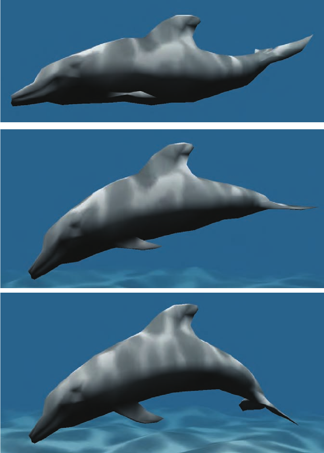
Figure 4.13. Vertex morphing. Two locations and normals are defined for every vertex.
In each frame, the intermediate location and normal are linearly interpolated by the
vertex shader. (Images courtesy of NVIDIA Corporation.)

i
i
i
i
i
i
i
i
4.5. Morphing 87
neutral smiling difference vectors
Figure 4.14. Given two mouth poses, a set of difference vectors is computed to control
interpolation, or even extrapolation. In morph targets, the difference vectors are used to
“add” movements onto the neutral face. With positive weights for the difference vectors,
we get a smiling mouth, while negative weights can give the opposite effect.
We start out with a neutral model, which in this case is a face. Let us
denote this model by N. In addition, we also have a set of different face
poses. In the example illustration, there is only one pose, which is a smiling
face. In general, we can allow k ≥ 1 different poses, which are denoted P
i
,
i ∈ [1,...,k]. As a preprocess, the “difference faces” are computed as:
D
i
= P
i
−N, i.e., the neutral model is subtracted from each pose.
At this point, we have a neutral model, N, and a set of difference poses,
D
i
. A morphed model M can then be obtained using the following formula:
M = N +
k
i=1
w
i
D
i
. (4.58)
This is the neutral model, and on top of that we add the features of the
different poses as desired, using the weights, w
i
. For Figure 4.14, setting
w
1
= 1 gives us exactly the smiling face in the middle of the illustration.
Using w
1
=0.5 gives us a half-smiling face, and so on. One can also use
negative weights and weights greater than one.
For this simple face model, we could add another face having “sad”
eyebrows. Using a negative weight for the eyebrows could then create
“happy” eyebrows. Since displacements are additive, this eyebrow pose
could be used in conjunction with the pose for a smiling mouth. Morph
targets are a powerful technique that provides the animator with much
control, since different features of a model can be manipulated indepen-
dently of the others. Lewis et al. [770] introduce pose-space deformation,
which combines vertex blending and morph targets. Hardware supporting
DirectX 10 can use stream-out and other improved functionality to allow
..................Content has been hidden....................
You can't read the all page of ebook, please click here login for view all page.