
Chapter 9
Multiple Regression and Model Building
9.1 An Example of Multiple Regression
Chapter 8 examined regression modeling for the simple linear regression case of a single predictor and a single response. Clearly, however, data miners and predictive analysts are usually interested in the relationship between the target variable and a set of (two or more) predictor variables. Most data mining applications enjoy a wealth of data, with some data sets including hundreds or thousands of variables, many of which may have a linear relationship with the target (response) variable. Multiple regression modeling provides an elegant method of describing such relationships. Compared to simple linear regression, multiple regression models provide improved precision for estimation and prediction, analogous to the improved precision of regression estimates over univariate estimates. A multiple regression model uses a linear surface, such as a plane or hyperplane, to approximate the relationship between a continuous response (target) variable, and a set of predictor variables. While the predictor variables are typically continuous, categorical predictor variables may be included as well, through the use of indicator (dummy) variables.
In simple linear regression, we used a straight line (of dimension 1) to approximate the relationship between the response and one predictor. Now, suppose we would like to approximate the relationship between a response and two continuous predictors. In this case, we would need a plane to approximate such a relationship, because a plane is linear in two dimensions.
For example, returning to the cereals data set, suppose we are interested in trying to estimate the value of the target variable, nutritional rating, but this time using two variables, sugars and fiber, rather than sugars alone as in Chapter 8.1 The three-dimensional scatter plot of the data is shown in Figure 9.1. High fiber levels seem to be associated with high nutritional rating, while high sugar levels seem to be associated with low nutritional rating.

Figure 9.1 A plane approximates the linear relationship between one response and two continuous predictors.
These relationships are approximated by the plane that is shown in Figure 9.1, in a manner analogous to the straight-line approximation for simple linear regression. The plane tilts downward to the right (for high sugar levels) and toward the front (for low fiber levels).
We may also examine the relationship between rating and its predictors, sugars, and fiber, one at a time, as shown in Figure 9.2. This more clearly illustrates the negative relationship between rating and sugars and the positive relationship between rating and fiber. The multiple regression should reflect these relationships.

Figure 9.2 Individual variable scatter plots of rating versus sugars and fiber.
Let us examine the results (Table 9.1) of a multiple regression of nutritional rating on both predictor variables. The regression equation for multiple regression with two predictor variables takes the form:
For a multiple regression with m variables, the regression equation takes the form:
From Table 9.1, we have
Thus, the regression equation for this example is
That is, the estimated nutritional rating equals 52.174 minus 2.2436 times the grams of sugar plus 2.8665 times the grams of fiber. Note that the coefficient for sugars is negative, indicating a negative relationship between sugars and rating, while the coefficient for fiber is positive, indicating a positive relationship. These results concur with the characteristics of the graphs in Figures 9.1 and 9.2. The straight lines shown in Figure 9.2 represent the value of the slope coefficients for each variable, −2.2436 for sugars and 2.8665 for fiber.
Table 9.1 Results from regression of nutritional rating on sugars and fiber
 |
The interpretations of the slope coefficients ![]() and
and ![]() are slightly different than for the simple linear regression case. For example, to interpret
are slightly different than for the simple linear regression case. For example, to interpret ![]() , we say that “the estimated decrease in nutritional rating for a unit increase in sugar content is 2.2436 points, when fiber content is held constant.” Similarly, we interpret
, we say that “the estimated decrease in nutritional rating for a unit increase in sugar content is 2.2436 points, when fiber content is held constant.” Similarly, we interpret ![]() as follows: “the estimated increase in nutritional rating for a unit increase in fiber content is 2.8408 points, when sugar content is held constant.” In general, for a multiple regression with m predictor variables, we would interpret coefficient
as follows: “the estimated increase in nutritional rating for a unit increase in fiber content is 2.8408 points, when sugar content is held constant.” In general, for a multiple regression with m predictor variables, we would interpret coefficient ![]() as follows: “the estimated change in the response variable for a unit increase in variable
as follows: “the estimated change in the response variable for a unit increase in variable ![]() is
is ![]() , when all other predictor variables are held constant.”
, when all other predictor variables are held constant.”
Recall that errors in prediction are measured by the residual, ![]() . In simple linear regression, this residual represented the vertical distance between the actual data point and the regression line. In multiple regression, the residual is represented by the vertical distance between the data point and the regression plane or hyperplane.
. In simple linear regression, this residual represented the vertical distance between the actual data point and the regression line. In multiple regression, the residual is represented by the vertical distance between the data point and the regression plane or hyperplane.
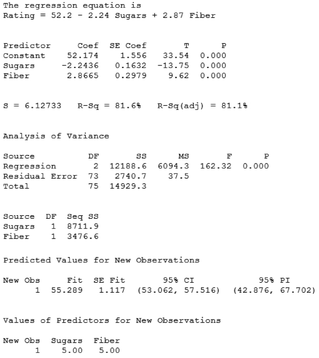
For example, Spoon Size Shredded Wheat has ![]() grams of sugar,
grams of sugar, ![]() grams of fiber, and a nutritional rating of 72.8018. The estimated regression equation would predict, however, that the nutritional rating for this cereal would be
grams of fiber, and a nutritional rating of 72.8018. The estimated regression equation would predict, however, that the nutritional rating for this cereal would be
Therefore, we have a residual for Spoon Size Shredded Wheat of ![]() , illustrated in Figure 9.3. As the residual is positive, the data value lies above the regression plane.
, illustrated in Figure 9.3. As the residual is positive, the data value lies above the regression plane.
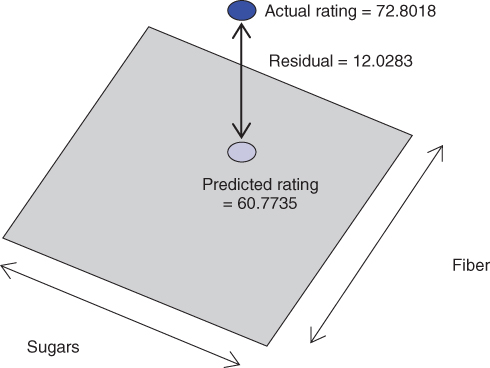
Figure 9.3 Estimation error is the vertical distance between the actual data point and the regression plane or hyperplane.
Each observation has its own residual, which, taken together, leads to the calculation of the sum of squares error (SSE) as an overall measure of the estimation errors. Just as for the simple linear regression case, we may again calculate the three sums of squares, as follows:
We may again present the regression statistics succinctly in a convenient analysis of variance (ANOVA) table, shown here in Table 9.2, where m represents the number of predictor variables. Finally, for multiple regression, we have the so-called multiple coefficient of determination,2 which is simply
For multiple regression, ![]() is interpreted as the proportion of the variability in the target variable that is accounted for by its linear relationship with the set of predictor variables.
is interpreted as the proportion of the variability in the target variable that is accounted for by its linear relationship with the set of predictor variables.
Table 9.2 The ANOVA table for multiple regression
| Source of Variation | Sum of Squares | Degrees of Freedom | Mean Square | F |
| Regression | SSR | m | ||
| Error (or residual) | SSE | |||
| Total |
From Table 9.1, we can see that the value of ![]() is 81.6%, which means that 81.6% of the variability in nutritional rating is accounted for by the linear relationship (the plane) between rating and the set of predictors, sugar content and fiber content. Now, would we expect
is 81.6%, which means that 81.6% of the variability in nutritional rating is accounted for by the linear relationship (the plane) between rating and the set of predictors, sugar content and fiber content. Now, would we expect ![]() to be greater than the value for the coefficient of determination we got from the simple linear regression of nutritional rating on sugars alone? The answer is yes. Whenever a new predictor variable is added to the model, the value of
to be greater than the value for the coefficient of determination we got from the simple linear regression of nutritional rating on sugars alone? The answer is yes. Whenever a new predictor variable is added to the model, the value of ![]() always goes up. If the new variable is useful, the value of
always goes up. If the new variable is useful, the value of ![]() will increase significantly; if the new variable is not useful, the value of
will increase significantly; if the new variable is not useful, the value of ![]() may barely increase at all.
may barely increase at all.
Table 8.7, here reproduced as Table 9.3, provides us with the coefficient of determination for the simple linear regression case, ![]() . Thus, by adding the new predictor, fiber content, to the model, we can account for an additional
. Thus, by adding the new predictor, fiber content, to the model, we can account for an additional ![]() of the variability in the nutritional rating. This seems like a significant increase, but we shall defer this determination until later.
of the variability in the nutritional rating. This seems like a significant increase, but we shall defer this determination until later.
Table 9.3 Results for regression of nutritional rating versus sugar content alone
 |
The typical error in estimation is provided by the standard error of the estimate, s. The value of s here is about 6.13 rating points. Therefore, our estimation of the nutritional rating of the cereals, based on sugar and fiber content, is typically in error by about 6.13 points. Now, would we expect this error to be greater or less than the value for s obtained by the simple linear regression of nutritional rating on sugars alone? In general, the answer depends on the usefulness of the new predictor. If the new variable is useful, then s will decrease, but if the new variable is not useful for predicting the target variable, then s may in fact increase. This type of behavior makes s, the standard error of the estimate, a more attractive indicator than ![]() of whether a new variable should be added to the model, because
of whether a new variable should be added to the model, because ![]() always increases when a new variable is added, regardless of its usefulness.
always increases when a new variable is added, regardless of its usefulness.
Table 9.3 shows that the value for s from the regression of rating on sugars alone was about 9.17. Thus, the addition of fiber content as a predictor decreased the typical error in estimating nutritional content from 9.17 points to 6.13 points, a decrease of 3.04 points. Thus, adding a second predictor to our regression analysis decreased the prediction error (or, equivalently, increased the precision) by about three points.
Next, before we turn to inference in multiple regression, we first examine the details of the population multiple regression equation.
9.2 The Population Multiple Regression Equation
We have seen that, for simple linear regression, the regression model takes the form:
with ![]() and
and ![]() as the unknown values of the true regression coefficients, and
as the unknown values of the true regression coefficients, and ![]() the error term, with its associated assumption discussed in Chapter 8. The multiple regression model is a straightforward extension of the simple linear regression model in equation (9.1), as follows.
the error term, with its associated assumption discussed in Chapter 8. The multiple regression model is a straightforward extension of the simple linear regression model in equation (9.1), as follows.
Just as we did for the simple linear regression case, we can derive four implications for the behavior of the response variable, y, as follows.
9.3 Inference in Multiple Regression
We shall examine five inferential methods in this chapter, which are as follows:
- The t-test for the relationship between the response variable
 and a particular predictor variable
  , in the presence of the other predictor variables,
  , where
  denotes the set of all predictors, not including
  .
. - The F-test for the significance of the regression as a whole.
- The confidence interval,
 , for the slope of the ith predictor variable.
 - The confidence interval for the mean of the response variable
 , given a set of particular values for the predictor variables
  .
. - The prediction interval for a random value of the response variable
 , given a set of particular values for the predictor variables
  .
.
9.3.1 The t-Test for the Relationship Between y and xi
The hypotheses for this test are given by
The models implied by these hypotheses are given by
Note that the only difference between the two models is the presence or absence of the ith term. All other terms are the same in both models. Therefore, interpretations of the results for this t-test must include some reference to the other predictor variables being held constant.
Under the null hypothesis, the test statistic ![]() follows a t distribution with n − m − 1 degrees of freedom, where
follows a t distribution with n − m − 1 degrees of freedom, where ![]() refers to the standard error of the slope for the ith predictor variable. We proceed to perform the t-test for each of the predictor variables in turn, using the results displayed in Table 9.1.
refers to the standard error of the slope for the ith predictor variable. We proceed to perform the t-test for each of the predictor variables in turn, using the results displayed in Table 9.1.
9.3.2 t-Test for Relationship Between Nutritional Rating and Sugars


- In Table 9.1, under “Coef” in the “Sugars” row is found the value,
 .
. - Under “SE Coef” in the “Sugars” row is found the value of the standard error of the slope for sugar content,
 .
. - Under “T” is found the value of the t-statistic; that is, the test statistic for the t-test,
 .
. - Under “P” is found the p-value of the t-statistic. As this is a two-tailed test, this p-value takes the following form:
 , where
  represents the observed value of the t-statistic from the regression results. Here,
  , although, of course, no continuous p-value ever precisely equals zero.
The p-value method is used, whereby the null hypothesis is rejected when the p-value of the test statistic is small. Here, we have p-value ![]() , which is smaller than any reasonable threshold of significance. Our conclusion is therefore to reject the null hypothesis. The interpretation of this conclusion is that there is evidence for a linear relationship between nutritional rating and sugar content, in the presence of fiber content.
, which is smaller than any reasonable threshold of significance. Our conclusion is therefore to reject the null hypothesis. The interpretation of this conclusion is that there is evidence for a linear relationship between nutritional rating and sugar content, in the presence of fiber content.
9.3.3 t-Test for Relationship Between Nutritional Rating and Fiber Content


- In Table 9.1, under “Coef” in the “Fibers” row is found the value,
 .
. - Under “SE Coef” in the “Fiber” row is found the value of the standard error of the slope for fiber,
 .
. - Under “T” is found the test statistic for the t-test,
 .
. - Under “P” is found the p-value of the t-statistic. Again,
 .
.
Thus, our conclusion is again to reject the null hypothesis. We interpret this to mean that there is evidence for a linear relationship between nutritional rating and fiber content, in the presence of sugar content.
9.3.4 The F-Test for the Significance of the Overall Regression Model
Next, we introduce the F-test for the significance of the overall regression model. Figure 9.4 illustrates the difference between the t-test and the F-test. One may apply a separate t-test for each predictor ![]() , or
, or ![]() , examining whether a linear relationship exists between the target variable y and that particular predictor. However, the F-test considers the linear relationship between the target variable y and the set of predictors (e.g.,
, examining whether a linear relationship exists between the target variable y and that particular predictor. However, the F-test considers the linear relationship between the target variable y and the set of predictors (e.g., ![]() ), taken as a whole.
), taken as a whole.
Figure 9.4 The F-test considers the relationship between the target and the set of predictors, taken as a whole.
The hypotheses for the F-test are given by

The null hypothesis asserts that there is no linear relationship between the target variable y, and the set of predictors, ![]() . Thus, the null hypothesis states that the coefficient
. Thus, the null hypothesis states that the coefficient ![]() for each predictor
for each predictor ![]() exactly equals zero, leaving the null model to be
exactly equals zero, leaving the null model to be
The alternative hypothesis does not assert that all the regression coefficients differ from zero. For the alternative hypothesis to be true, it is sufficient for a single, unspecified, regression coefficient to differ from zero. Hence, the alternative hypothesis for the F-test does not specify a particular model, because it would be true if any, some, or all of the coefficients differed from zero.
As shown in Table 9.2, the F-statistic consists of a ratio of two means squares, the mean square regression (MSR) and the mean square error (MSE). A mean square represents a sum of squares divided by the degrees of freedom associated with that sum of squares statistic. As the sums of squares are always nonnegative, then so are the mean squares. To understand how the F-test works, we should consider the following.
The MSE is always a good estimate of the overall variance (see model assumption 2) ![]() , regardless of whether the null hypothesis is true or not. (In fact, recall that we use the standard error of the estimate,
, regardless of whether the null hypothesis is true or not. (In fact, recall that we use the standard error of the estimate, ![]() , as a measure of the usefulness of the regression, without reference to an inferential model.) Now, the MSR is also a good estimate of
, as a measure of the usefulness of the regression, without reference to an inferential model.) Now, the MSR is also a good estimate of ![]() , but only on the condition that the null hypothesis is true. If the null hypothesis is false, then MSR overestimates
, but only on the condition that the null hypothesis is true. If the null hypothesis is false, then MSR overestimates ![]() .
.
So, consider the value of ![]() , with respect to the null hypothesis. Suppose MSR and MSE are close to each other, so that the value of F is small (near 1.0). As MSE is always a good estimate of
, with respect to the null hypothesis. Suppose MSR and MSE are close to each other, so that the value of F is small (near 1.0). As MSE is always a good estimate of ![]() , and MSR is only a good estimate of
, and MSR is only a good estimate of ![]() when the null hypothesis is true, then the circumstance that MSR and MSE are close to each other will only occur when the null hypothesis is true. Therefore, when the value of F is small, this is evidence that the null hypothesis is true.
when the null hypothesis is true, then the circumstance that MSR and MSE are close to each other will only occur when the null hypothesis is true. Therefore, when the value of F is small, this is evidence that the null hypothesis is true.
However, suppose that MSR is much greater than MSE, so that the value of F is large. MSR is large (overestimates ![]() ) when the null hypothesis is false. Therefore, when the value of F is large, this is evidence that the null hypothesis is false. Therefore, for the F-test, we shall reject the null hypothesis when the value of the test statistic F is large.
) when the null hypothesis is false. Therefore, when the value of F is large, this is evidence that the null hypothesis is false. Therefore, for the F-test, we shall reject the null hypothesis when the value of the test statistic F is large.
The observed F-statistic ![]() follows an
follows an ![]() distribution. As all F values are nonnegative, the F-test is a right-tailed test. Thus, we will reject the null hypothesis when the p-value is small, where the p-value is the area in the tail to the right of the observed F statistic. That is,
distribution. As all F values are nonnegative, the F-test is a right-tailed test. Thus, we will reject the null hypothesis when the p-value is small, where the p-value is the area in the tail to the right of the observed F statistic. That is, ![]() , and we reject the null hypothesis when
, and we reject the null hypothesis when ![]() is small.
is small.
9.3.5 F-Test for Relationship Between Nutritional Rating and {Sugar and Fiber}, Taken Together
 .
.
- The model implied by Ha is not specified, and may be any one of the following:

 .
.
- In Table 9.1, under “MS” in the “Regression” row of the “Analysis of Variance” table, is found the value of MSR, 6094.3.
- Under “MS” in the “Residual Error” row of the “Analysis of Variance” table is found the value of MSE, 37.5.
- Under “F” in the “Regression” row of the “Analysis of Variance” table is found the value of the test statistic
 .
. - The degrees of freedom for the F-statistic are given in the column marked “DF,” so that we have
 , and
, and  .
. - Under “P” in the “Regression” row of the “Analysis of Variance” table is found the p-value of the F-statistic. Here, the p-value is
 , although again no continuous p-value ever precisely equals zero.
This p-value of approximately zero is less than any reasonable threshold of significance. Our conclusion is therefore to reject the null hypothesis. The interpretation of this conclusion is the following. There is evidence for a linear relationship between nutritional rating on the one hand, and the set of predictors, sugar content and fiber content, on the other. More succinctly, we may simply say that the overall regression model is significant.
9.3.6 The Confidence Interval for a Particular Coefficient, βi
Just as for simple linear regression, we may construct a ![]() confidence interval for a particular coefficient,
confidence interval for a particular coefficient, ![]() , as follows. We can be
, as follows. We can be ![]() confident that the true value of a particular coefficient
confident that the true value of a particular coefficient ![]() lies within the following interval:
lies within the following interval:
where ![]() is based on
is based on ![]() degrees of freedom, and
degrees of freedom, and ![]() represents the standard error of the ith coefficient estimate.
represents the standard error of the ith coefficient estimate.
For example, let us construct a 95% confidence interval for the true value of the coefficient ![]() for
for ![]() , sugar content. From Table 9.1, the point estimate is given as
, sugar content. From Table 9.1, the point estimate is given as ![]() . The t-critical value for 95% confidence and
. The t-critical value for 95% confidence and ![]() degrees of freedom is
degrees of freedom is ![]() . The standard error of the coefficient estimate is
. The standard error of the coefficient estimate is ![]() . Thus, our confidence interval is as follows:
. Thus, our confidence interval is as follows:

We are 95% confident that the value for the coefficient ![]() lies between −2.57 and −1.92. In other words, for every additional gram of sugar, the nutritional rating will decrease by between 1.92 and 2.57 points, when fiber content is held constant. For example, suppose a nutrition researcher claimed that nutritional rating would fall two points for every additional gram of sugar, when fiber is held constant. As −2.0 lies within the 95% confidence interval, then we would not reject this hypothesis, with 95% confidence.
lies between −2.57 and −1.92. In other words, for every additional gram of sugar, the nutritional rating will decrease by between 1.92 and 2.57 points, when fiber content is held constant. For example, suppose a nutrition researcher claimed that nutritional rating would fall two points for every additional gram of sugar, when fiber is held constant. As −2.0 lies within the 95% confidence interval, then we would not reject this hypothesis, with 95% confidence.
9.3.7 The Confidence Interval for the Mean Value of y, Given x1, x2, …, xm
We may find confidence intervals for the mean value of the target variable y, given a particular set of values for the predictors ![]() . The formula is a multivariate extension of the analogous formula from Chapter 8, requires matrix multiplication, and may be found in Draper and Smith.3 For example, the bottom of Table 9.1 (“Values of Predictors for New Observations”) shows that we are interested in finding the confidence interval for the mean of the distribution of all nutritional ratings, when the cereal contains 5.00 grams of sugar and 5.00 grams of fiber.
. The formula is a multivariate extension of the analogous formula from Chapter 8, requires matrix multiplication, and may be found in Draper and Smith.3 For example, the bottom of Table 9.1 (“Values of Predictors for New Observations”) shows that we are interested in finding the confidence interval for the mean of the distribution of all nutritional ratings, when the cereal contains 5.00 grams of sugar and 5.00 grams of fiber.
The resulting 95% confidence interval is given, under “Predicted Values for New Observations,” as “95% CI” = (53.062, 57.516). That is, we can be 95% confident that the mean nutritional rating of all cereals with 5.00 grams of sugar and 5.00 grams of fiber lies between 55.062 points and 57.516 points.
9.3.8 The Prediction Interval for a Randomly Chosen Value of y, Given x1, x2, …, xm
Similarly, we may find a prediction interval for a randomly selected value of the target variable, given a particular set of values for the predictors ![]() . We refer to Table 9.1 for our example of interest: 5.00 grams of sugar and 5.00 grams of fiber. Under “95% PI,” we find the prediction interval to be (42,876, 67.702). In other words, we can be 95% confident that the nutritional rating for a randomly chosen cereal with 5.00 grams of sugar and 5.00 grams of fiber lies between 42.876 points and 67.702 points. Again, note that the prediction interval is wider than the confidence interval, as expected.
. We refer to Table 9.1 for our example of interest: 5.00 grams of sugar and 5.00 grams of fiber. Under “95% PI,” we find the prediction interval to be (42,876, 67.702). In other words, we can be 95% confident that the nutritional rating for a randomly chosen cereal with 5.00 grams of sugar and 5.00 grams of fiber lies between 42.876 points and 67.702 points. Again, note that the prediction interval is wider than the confidence interval, as expected.
9.4 Regression With Categorical Predictors, Using Indicator Variables
Thus far, our predictors have all been continuous. However, categorical predictor variables may also be used as inputs to regression models, through the use of indicator variables (dummy variables). For example, in the cereals data set, consider the variable shelf, which indicates which supermarket shelf the particular cereal was located on. Of the 76 cereals, 19 were located on shelf 1, 21 were located on shelf 2, and 36 were located on shelf 3.
A dot plot of the nutritional rating for the cereals on each shelf is provided in Figure 9.5, with the shelf means indicated by the triangles. Now, if we were to use only the categorical variables (such as shelf and manufacturer) as predictors, then we could perform ANOVA.4 However, we are interested in using the categorical variable shelf along with continuous variables such as sugar content and fiber content. Therefore, we shall use multiple regression analysis with indicator variables.

Figure 9.5 Is there evidence that shelf location affects nutritional rating?
On the basis of comparison dot plot in Figure 9.5, does there seem to be evidence that shelf location affects nutritional rating? It would seem that shelf 2 cereals, with their average nutritional rating of 34.97, seem to lag somewhat behind the cereals on shelf 1 and shelf 3, with their respective average nutritional ratings of 45.90 and 45.22. However, it is not clear whether this difference is significant. Further, this dot plot does not take into account the other variables, such as sugar content and fiber
content; it is unclear how any “shelf effect” would manifest itself, in the presence of these other variables.
For use in regression, a categorical variable with k categories must be transformed into a set of k − 1 indicator variables. An indicator variable, also known as a flag variable, or a dummy variable, is a binary 0/1 variable, which takes the value 1 if the observation belongs to the given category, and takes the value 0 otherwise.
For the present example, we define the following indicator variables:


Table 9.4 indicates the values taken by these indicator variables, for cereals located on shelves 1, 2, and 3, respectively. Note that it is not necessary to define a third indicator variable “shelf 3,” because cereals located on shelf 3 will have zero values for each of the shelf 1 and shelf 2 indicator variables, and this is sufficient to distinguish them. In fact, one should not define this third dummy variable because the resulting covariate matrix will be singular, and the regression will not work. The category that is not assigned an indicator variable is denoted the reference category. Here, shelf 3 is the reference category. Later, we shall measure the effect of the location of a given cereal (e.g., on shelf 1) on nutritional rating, with respect to (i.e., with reference to) shelf 3, the reference category.
Table 9.4 Values taken by the indicator variables, for cereals located on shelves 1, 2, and 3, respectively
| Cereal Location | Value of Variable Shelf 1 | Value of Variable Shelf 2 |
| Shelf 1 | 1 | 0 |
| Shelf 2 | 0 | 1 |
| Shelf 3 | 0 | 0 |
So, let us construct a multiple regression model using only the two indicator variables shown in Table 9.4. In this case, our regression equation is
Before we run the regression, let us think about what the regression coefficient values might be. On the basis of Figure 9.5, we would expect ![]() to be negative, because the shelf 2 cereals have a lower mean rating, compared to shelf 3 cereals. We might also expect
to be negative, because the shelf 2 cereals have a lower mean rating, compared to shelf 3 cereals. We might also expect ![]() to be essentially negligible but slightly positive, reflecting the slightly greater mean rating for shelf 1 cereals, compared to with shelf 3 cereals.
to be essentially negligible but slightly positive, reflecting the slightly greater mean rating for shelf 1 cereals, compared to with shelf 3 cereals.
Table 9.5 contains the results of the regression of nutritional rating on shelf 1 and shelf 2 only. Note that the coefficient for the shelf 2 dummy variable is −10.247, which is equal (after rounding) to the difference in the mean nutritional ratings between cereals on shelves 2 and 3: 34.97 − 45.22. Similarly, the coefficient for the shelf 1 dummy variable is 0.679, which equals (after rounding) the difference in the mean ratings between cereals on shelves 1 and 3: 45.90 − 45.22. These values fulfill our expectations, based on Figure 9.5.
Table 9.5 Results of regression of nutritional rating on shelf location only
 |
Next, let us proceed to perform multiple regression, for the linear relationship between nutritional rating and sugar content, fiber content, and shelf location, using the two dummy variables from Table 9.4. The regression equation is given as
For cereals located on shelf 1, regression equation looks like the following:
For cereals located on shelf 2, the regression equation is
Finally, for cereals located on shelf 3, the regression equation is as follows:
Note the relationship of the model equations to each other. The three models represent parallel planes, as illustrated in Figure 9.6. (Note that the planes do not, of course, directly represent the shelves themselves, but the fit of the regression model to the nutritional rating, for the cereals on the various shelves.) The results for the regression of nutritional rating on sugar content, fiber content, and shelf location are provided in Table 9.6. The general form of the regression equation looks like:
Thus, the regression equation for cereals located on the various shelves is given as the following:

Note that these estimated regression equations are exactly the same, except for the y-intercept. This means that cereals on each shelf are modeled as following the exact same slope in the sugars dimension (−2.3183) and the exact same slope in the fiber dimension (3.1314), which gives us the three parallel planes shown in Figure 9.6. The only difference lies in the value of the y-intercept for the cereals on the three shelves.
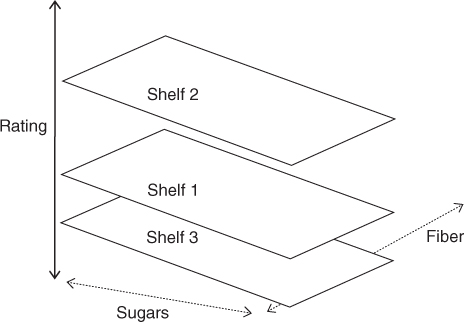
Figure 9.6 The use of indicator variables in multiple regression leads to a set of parallel planes (or hyperplanes).
Table 9.6 Results for the regression of nutritional rating on sugar content, fiber content, and shelf location
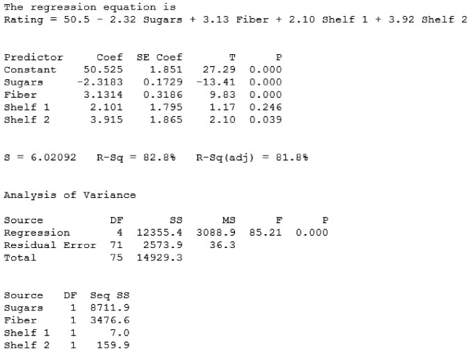 |
The reference category in this case is shelf 3. What is the vertical distance between the shelf 3 plane and, for example, the shelf 1 plane? Note from the derivations above that the estimated regression equation for the cereals on shelf 1 is given as
so that the y-intercept is ![]() . We also have the estimated regression equation for the cereals on shelf 3 to be
. We also have the estimated regression equation for the cereals on shelf 3 to be
Thus, the difference between the y-intercepts is ![]() . We can verify this by noting that
. We can verify this by noting that ![]() , which is the value of
, which is the value of ![]() reported in Table 9.6. The vertical distance between the planes representing shelves 1 and 3 is everywhere 2.101 rating points, as shown in Figure 9.7.
reported in Table 9.6. The vertical distance between the planes representing shelves 1 and 3 is everywhere 2.101 rating points, as shown in Figure 9.7.

Figure 9.7 The indicator variables coefficients estimate the difference in the response value, compared to the reference category.
Of particular importance is the interpretation of this value for ![]() . Now, the y-intercept represents the estimated nutritional rating when both sugars and fiber equal zero. However, as the planes are parallel, the difference in the y-intercepts among the shelves remains constant throughout the range of sugar and fiber values. Thus, the vertical distance between the parallel planes, as measured by the coefficient for the indicator variable, represents the estimated effect of the particular indicator variable on the target variable, with respect to the reference category.
. Now, the y-intercept represents the estimated nutritional rating when both sugars and fiber equal zero. However, as the planes are parallel, the difference in the y-intercepts among the shelves remains constant throughout the range of sugar and fiber values. Thus, the vertical distance between the parallel planes, as measured by the coefficient for the indicator variable, represents the estimated effect of the particular indicator variable on the target variable, with respect to the reference category.
In this example, ![]() represents the estimated difference in nutritional rating for cereals located on shelf 1, compared to the cereals on shelf 3. As
represents the estimated difference in nutritional rating for cereals located on shelf 1, compared to the cereals on shelf 3. As ![]() is positive, this indicates that the estimated nutritional rating for shelf 1 cereals is higher. We thus interpret
is positive, this indicates that the estimated nutritional rating for shelf 1 cereals is higher. We thus interpret ![]() as follows: The estimated increase in nutritional rating for cereals located on shelf 1, as compared to cereals located on shelf 3, is
as follows: The estimated increase in nutritional rating for cereals located on shelf 1, as compared to cereals located on shelf 3, is ![]() points, when sugars and fiber content are held constant. It is similar for the cereals on shelf 2. We have the estimated regression equation for these cereals as:
points, when sugars and fiber content are held constant. It is similar for the cereals on shelf 2. We have the estimated regression equation for these cereals as:
so that the difference between the y-intercepts for the planes representing shelves 2 and 3 is ![]() . We thus have
. We thus have ![]() , which is the value for
, which is the value for ![]() reported in Table 9.6. That is, the vertical distance between the planes representing shelves 2 and 3 is everywhere 3.915 rating points, as shown in Figure 9.7. Therefore, the estimated increase in nutritional rating for cereals located on shelf 2, as compared to cereals located on shelf 3, is
reported in Table 9.6. That is, the vertical distance between the planes representing shelves 2 and 3 is everywhere 3.915 rating points, as shown in Figure 9.7. Therefore, the estimated increase in nutritional rating for cereals located on shelf 2, as compared to cereals located on shelf 3, is ![]() points, when sugars and fiber content are held constant.
points, when sugars and fiber content are held constant.
We may then infer the estimated difference in nutritional rating between shelves 2 and 1. This is given as ![]() points. The estimated increase in nutritional rating for cereals located on shelf 2, as compared to cereals located on shelf 1, is 1.814 points, when sugars and fiber content are held constant.
points. The estimated increase in nutritional rating for cereals located on shelf 2, as compared to cereals located on shelf 1, is 1.814 points, when sugars and fiber content are held constant.
Now, recall Figure 9.5, where we encountered evidence that shelf 2 cereals had the lowest nutritional rating, with an average of about 35, compared to average ratings of 46 and 45 for the cereals on the other shelves. How can this knowledge be reconciled with the dummy variable results, which seem to show the highest rating for shelf 2?
The answer is that our indicator variable results are accounting for the presence of the other variables, sugar content and fiber content. It is true that the cereals on shelf 2 have the lowest nutritional rating; however, as shown in Table 9.7, these cereals also have the highest sugar content (average 9.62 grams, compared to 5.11 and 6.53 grams for shelves 1 and 3) and the lowest fiber content (average 0.91 grams, compared to 1.63 and 3.14 grams for shelves 1 and 3). Because of the negative correlation between sugar and rating, and the positive correlation between fiber and rating, the shelf 2 cereals already have a relatively low estimated nutritional rating based on these two predictors alone.
Table 9.7 Using sugars and fiber only, the regression model underestimates the nutritional rating of shelf 2 cereals
| Shelf | Mean Sugars | Mean Fiber | Mean Rating | Mean Estimated Ratinga | Mean Error |
| 1 | 5.11 | 1.63 | 45.90 | 45.40 | −0.50 |
| 2 | 9.62 | 0.91 | 34.97 | 33.19 | −1.78 |
| 3 | 6.53 | 3.14 | 45.22 | 46.53 | +1.31 |
a Rating estimated using sugars and fiber only, and not shelf location.5
Table 9.7 shows the mean fitted values (estimated ratings) for the cereals on the various shelves, when sugar and fiber content are included in the model, but shelf location is not included as a predictor. Note that, on average, the nutritional rating of the shelf 2 cereals is underestimated by 1.78 points. However, the nutritional rating of the shelf 3 cereals is overestimated by 1.31 points. Therefore, when shelf location is introduced into the model, these over-/underestimates can be compensated for. Note from Table 9.7 that the relative estimation error difference between shelves 2 and 3 is 1.31 + 1.78 = 3.09. Thus, we would expect that if shelf location were going to compensate for the underestimate of shelf 2 cereals relative to shelf 3 cereals, it would add a factor in the neighborhood of 3.09 ratings points. Recall from Figure 9.6 that ![]() , which is in the ballpark of 3.09. Also, note that the relative estimation error difference between shelves 1 and 3 is 1.31 + 0.50 = 1.81. We would expect that the shelf indicator variable compensating for this estimation error would be not far from 1.81, and, indeed, we have the relevant coefficient as
, which is in the ballpark of 3.09. Also, note that the relative estimation error difference between shelves 1 and 3 is 1.31 + 0.50 = 1.81. We would expect that the shelf indicator variable compensating for this estimation error would be not far from 1.81, and, indeed, we have the relevant coefficient as ![]() .
.
This example illustrates the flavor of working with multiple regression, in that the relationship of the set of predictors with the target variable is not necessarily dictated by the individual bivariate relationships the target variable has with each of the predictors. For example, Figure 9.5 would have led us to believe that shelf 2 cereals would have had an indicator variable adjusting the estimated nutritional rating downward. But the actual multiple regression model, which included sugars, fiber, and shelf location, had an indicator variable adjusting the estimated nutritional rating upward, because of the effects of the other predictors.
Consider again Table 9.6. Note that the p-values for the sugars coefficient and the fiber coefficient are both quite small (near zero), so that we may include both of these predictors in the model. However, the p-value for the shelf 1 coefficient is somewhat large (0.246), indicating that the relationship between this variable is not statistically significant. In other words, in the presence of sugars and fiber content, the difference in nutritional rating between shelf 1 cereals and shelf 3 cereals is not significant. We may therefore consider eliminating the shelf 1 indicator variable from the model. Suppose we go ahead and eliminate the shelf 1 indicator variable from the model, because of its large p-value, but retain the shelf 2 indicator variable. The results from the regression of nutritional rating on sugar content, fiber content, and shelf 2 (compared to shelf 3) location are given in Table 9.8.
Table 9.8 Results from regression of nutritional rating on sugars, fiber, and the shelf 2 indicator variable
 |
Note from Table 9.8 that the p-value for the shelf 2 dummy variable has increased from 0.039 to 0.077, indicating that it may no longer belong in the model. The effect of adding or removing predictors on the other predictors is not always predictable. This is why variable selection procedures exist to perform this task methodically, such as stepwise regression. We cover these methods later in this chapter.
9.5 Adjusting R2: Penalizing Models For Including Predictors That Are Not Useful
Recall that adding a variable to the model will increase the value of the coefficient of determination ![]() , regardless of the usefulness of the variable. This is not a particularly attractive feature of this measure, because it may lead us to prefer models with marginally larger values for
, regardless of the usefulness of the variable. This is not a particularly attractive feature of this measure, because it may lead us to prefer models with marginally larger values for ![]() , simply because they have more variables, and not because the extra variables are useful. Therefore, in the interests of parsimony, we should find some way to penalize the
, simply because they have more variables, and not because the extra variables are useful. Therefore, in the interests of parsimony, we should find some way to penalize the ![]() measure for models that include predictors that are not useful. Fortunately, such a penalized form for
measure for models that include predictors that are not useful. Fortunately, such a penalized form for ![]() does exist, and is known as the adjusted
does exist, and is known as the adjusted ![]() . The formula for adjusted
. The formula for adjusted ![]() is as follows:
is as follows:
If ![]() is much less than
is much less than ![]() , then this is an indication that at least one variable in the model may be extraneous, and the analyst should consider omitting that variable from the model.
, then this is an indication that at least one variable in the model may be extraneous, and the analyst should consider omitting that variable from the model.
As an example of calculating ![]() , consider Figure 9.8, where we have
, consider Figure 9.8, where we have


- n = 76
- m = 4
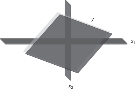
Figure 9.8 Matrix plot of the predictor variables shows correlation between fiber and potassium.
Then, ![]() .
.
Let us now compare Tables 9.6 and 9.8, where the regression model was run with and without the shelf 1 indicator variable, respectively. The shelf 1 indicator variable was found to be not useful for estimating nutritional rating. How did this affect ![]() and
and ![]() ?
?
- With shelf 1:

- Without shelf 1:

So, the regression model, not including shelf 1, suffers a smaller penalty than does the model that includes it, which would make sense if shelf 1 is not a helpful predictor. However, in this instance, the penalty is not very large in either case. Just remember: When one is building models in multiple regression, one should use ![]() and s, rather than the raw
and s, rather than the raw ![]() .
.
9.6 Sequential Sums of Squares
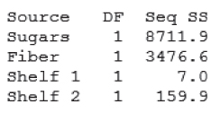
Some analysts use the information provided in the sequential sums of squares, provided by many software packages, to help them get a better idea of which variables to include in the model. The sequential sums of squares represent a partitioning of SSR, the regression sum of squares. Recall that SSR represents the proportion of the variability in the target variable that is explained by the linear relationship of the target variable with the set of predictor variables. The sequential sums of squares partition the SSR into the unique portions of the SSR that are explained by the particular predictors, given any earlier predictors. Thus, the values of the sequential sums of squares depend on the order that the variables are entered into the model. For example, the sequential sums of squares for the model:
are found in Table 9.6, and repeated here in Table 9.9. The sequential sum of squares shown for sugars is 8711.9, and represents the variability in nutritional rating that is explained by the linear relationship between rating and sugar content. In other words, this first sequential sum of squares is exactly the value for SSR from the simple linear regression of nutritional rating on sugar content.6
The second sequential sum of squares, for fiber content, equals 3476.6. This represents the amount of unique additional variability in nutritional rating that is explained by the linear relationship of rating with fiber content, given that the variability explained by sugars has already been extracted. The third sequential sum of squares, for shelf 1, is 7.0. This represents the amount of unique additional variability in nutritional rating that is accounted for by location on shelf 1 (compared to the reference class shelf 3), given that the variability accounted for by sugars and fiber has already been separated out. This tiny value for the sequential sum of squares for shelf 1 indicates that the variable is probably not useful for estimating nutritional rating. Finally, the sequential sum of squares for shelf 2 is a moderate 159.9.
Table 9.9 The sequential sums of squares for the model: y = β0 + β1(sugars) + β2(fiber) + β3(Shelf 1) + β4(Shelf 2) + ϵ
 |
Now, suppose we changed the ordering of the variables into the regression model. This would change the values of the sequential sums of squares. For example, suppose we perform an analysis based on the following model:
The results for this regression are provided in Table 9.10. Note that all the results in Table 9.10 are exactly the same as in Table 9.6 (apart from ordering), except the values of the sequential sums of squares. This time, the indicator variables are able to “claim” their unique portions of the variability before the other variables are entered, thus giving them larger values for their sequential sums of squares. See Neter, Wasserman, and Kutner7 for more information on applying sequential sums of squares for variable selection. We use the sequential sums of squares, in the context of a partial F-test, to perform variable selection later on in this chapter.
Table 9.10 Changing the ordering of the variables into the model changes nothing except the sequential sums of squares
 |
9.7 Multicollinearity
Suppose that we are now interested in adding the predictor potassium to the model, so that our new regression equation looks like:
Now, data miners need to guard against multicollinearity, a condition where some of the predictor variables are correlated with each other. Multicollinearity leads to instability in the solution space, leading to possible incoherent results. For example, in a data set with severe multicollinearity, it is possible for the F-test for the overall regression to be significant, while none of the t-tests for the individual predictors are significant.
Consider Figures 9.9 and 9.10. Figure 9.9 illustrates a situation where the predictors ![]() and
and ![]() are not correlated with each other; that is, they are orthogonal, or independent. In such a case, the predictors form a solid basis, on which the response surface y may rest sturdily, thereby providing stable coefficient estimates
are not correlated with each other; that is, they are orthogonal, or independent. In such a case, the predictors form a solid basis, on which the response surface y may rest sturdily, thereby providing stable coefficient estimates ![]() and
and ![]() , each with small variability
, each with small variability ![]() and
and ![]() . However, Figure 9.10 illustrates a multicollinear situation where the predictors
. However, Figure 9.10 illustrates a multicollinear situation where the predictors ![]() and
and ![]() are correlated with each other, so that as one of them increases, so does the other. In this case, the predictors no longer form a solid basis, on which the response surface may firmly rest. Instead, when the predictors are correlated, the response surface is unstable, providing highly variable coefficient estimates
are correlated with each other, so that as one of them increases, so does the other. In this case, the predictors no longer form a solid basis, on which the response surface may firmly rest. Instead, when the predictors are correlated, the response surface is unstable, providing highly variable coefficient estimates ![]() and
and ![]() , because of the inflated values for
, because of the inflated values for ![]() and
and ![]() .
.
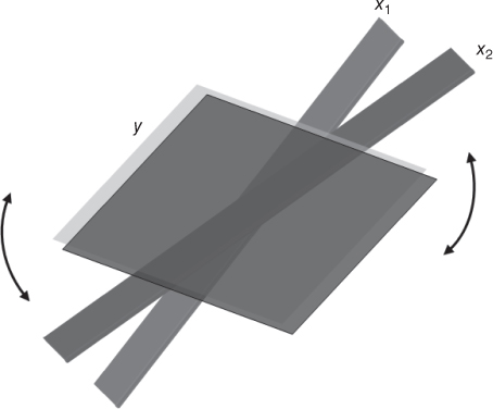
Figure 9.9 When the predictors  and
and  are uncorrelated, the response surface y rests on a solid basis, providing stable coefficient estimates.
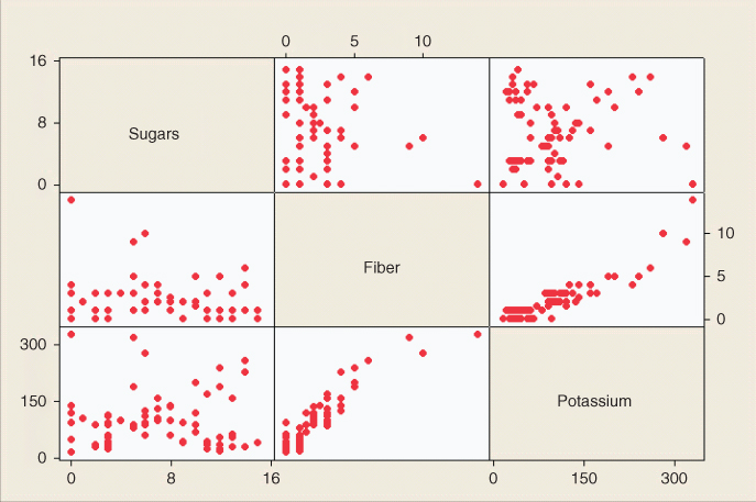
Figure 9.10 Multicollinearity: When the predictors are correlated, the response surface is unstable, resulting in dubious and highly variable coefficient estimates.
The high variability associated with the estimates means that different samples may produce coefficient estimates with widely different values. For example, one sample may produce a positive coefficient estimate for ![]() , while a second sample may produce a negative coefficient estimate. This situation is unacceptable when the analytic task calls for an explanation of the relationship between the response and the predictors, individually. Even if such instability is avoided, inclusion of variables that are highly correlated tends to overemphasize a particular component of the model, because the component is essentially being double counted.
, while a second sample may produce a negative coefficient estimate. This situation is unacceptable when the analytic task calls for an explanation of the relationship between the response and the predictors, individually. Even if such instability is avoided, inclusion of variables that are highly correlated tends to overemphasize a particular component of the model, because the component is essentially being double counted.
To avoid multicollinearity, the analyst should investigate the correlation structure among the predictor variables (ignoring for the moment the target variable). Table 9.118 provides the correlation coefficients among the predictors for our present model. For example, the correlation coefficient between sugars and fiber is −0.139, while the correlation coefficient between sugars and potassium is 0.001. Unfortunately, there is one pair of variables that are strongly correlated: fiber and potassium, with r = 0.912. Another method of assessing whether the predictors are correlated is to construct a matrix plot of the predictors, such as Figure 9.8. The matrix plot supports the finding that fiber and potassium are positively correlated.
Table 9.11 Correlation coefficients among the predictors: We have a problem
 |
However, suppose we did not check for the presence of correlation among our predictors, and went ahead and performed the regression anyway. Is there some way that the regression results can warn us of the presence of multicollinearity? The answer is yes: We may ask for the variance inflation factors (VIFs) to be reported.
What do we mean by VIFs? First, recall that ![]() represents the variability associated with the coefficient
represents the variability associated with the coefficient ![]() for the ith predictor variable
for the ith predictor variable ![]() . We may express
. We may express ![]() as a product of s, the standard error of the estimate, and
as a product of s, the standard error of the estimate, and ![]() , which is a constant whose value depends on the observed predictor values. That is,
, which is a constant whose value depends on the observed predictor values. That is, ![]() . Now, s is fairly robust with respect to the inclusion of correlated variables in the model, so, in the presence of correlated predictors, we would look to
. Now, s is fairly robust with respect to the inclusion of correlated variables in the model, so, in the presence of correlated predictors, we would look to ![]() to help explain large changes in
to help explain large changes in ![]() .
.
We may express ![]() as the following:
as the following:

where ![]() represents the sample variance of the observed values of ith predictor,
represents the sample variance of the observed values of ith predictor, ![]() , and
, and ![]() represents the
represents the ![]() value obtained by regressing
value obtained by regressing ![]() on the other predictor variables. Note that
on the other predictor variables. Note that ![]() will be large when
will be large when ![]() is highly correlated with the other predictors.
is highly correlated with the other predictors.
Note that, of the two terms in ![]() , the first factor
, the first factor ![]() measures only the intrinsic variability within the ith predictor,
measures only the intrinsic variability within the ith predictor, ![]() . It is the second factor
. It is the second factor ![]() that measures the correlation between the ith predictor
that measures the correlation between the ith predictor ![]() and the remaining predictor variables. For this reason, this second factor is denoted as the VIF for
and the remaining predictor variables. For this reason, this second factor is denoted as the VIF for ![]() :
:
Can we describe the behavior of the VIF? Suppose that ![]() is completely uncorrelated with the remaining predictors, so that
is completely uncorrelated with the remaining predictors, so that ![]() . Then we will have
. Then we will have ![]() . That is, the minimum value for VIF is 1, and is reached when
. That is, the minimum value for VIF is 1, and is reached when ![]() is completely uncorrelated with the remaining predictors. However, as the degree of correlation between
is completely uncorrelated with the remaining predictors. However, as the degree of correlation between ![]() and the other predictors increases,
and the other predictors increases, ![]() will also increase. In that case,
will also increase. In that case, ![]() will increase without bound, as
will increase without bound, as ![]() approaches 1. Thus, there is no upper limit to the value that
approaches 1. Thus, there is no upper limit to the value that ![]() can take.
can take.
What effect do these changes in ![]() have on
have on ![]() , the variability of the ith coefficient? We have
, the variability of the ith coefficient? We have ![]() . If
. If ![]() is uncorrelated with the other predictors, then
is uncorrelated with the other predictors, then ![]() , and the standard error of the coefficient
, and the standard error of the coefficient ![]() will not be inflated. However, if
will not be inflated. However, if ![]() is correlated with the other predictors, then the large
is correlated with the other predictors, then the large ![]() will produce an inflation of the standard error of the coefficient
will produce an inflation of the standard error of the coefficient ![]() . As you know, inflating the variance estimates will result in a degradation in the precision of the estimation. A rough rule of thumb for interpreting the value of the VIF is to consider
. As you know, inflating the variance estimates will result in a degradation in the precision of the estimation. A rough rule of thumb for interpreting the value of the VIF is to consider ![]() to be an indicator of moderate multicollinearity, and to consider
to be an indicator of moderate multicollinearity, and to consider ![]() to be an indicator of severe multicollinearity. A
to be an indicator of severe multicollinearity. A ![]() corresponds to
corresponds to ![]() , while
, while ![]() corresponds to
corresponds to ![]() .
.
Getting back to our example, suppose we went ahead with the regression of nutritional rating on sugars, fiber, the shelf 2 indicator, and the new variable potassium, which is correlated with fiber. The results, including the observed VIFs, are shown in Table 9.12. The estimated regression equation for this model is
The p-value for potassium is not very small (0.082), so at first glance, the variable may or may not be included in the model. Also, the p-value for the shelf 2 indicator variable (0.374) has increased to such an extent that we should perhaps not include it in the model. However, we should probably not put too much credence into any of these results, because the observed VIFs seem to indicate the presence of a multicollinearity problem. We need to resolve the evident multicollinearity before moving forward with this model.
Table 9.12 Regression results, with variance inflation factors indicating a multicollinearity problem
 |
Note that only 74 cases were used, because the potassium content of Almond Delight and Cream of Wheat are missing, along with the sugar content of Quaker Oats.
The VIF for fiber is 6.952 and the VIF for potassium is 7.157, with both values indicating moderate-to-strong multicollinearity. At least the problem is localized with these two variables only, as the other VIFs are reported at acceptably low values.
How shall we deal with this problem? Some texts suggest choosing one of the variables and eliminating it from the model. However, this should be viewed only as a last resort, because the omitted variable may have something to teach us. As we saw in Chapter 4, principal components can be a powerful method for using the correlation structure in a large group of predictors to produce a smaller set of independent components. Principal components analysis is a definite option here. Another option might be to construct a user-defined composite, as discussed in Chapter 4. Here, our user-defined composite will be as simple as possible, the mean of fiberz and potassiumz, where the z-subscript notation indicates that the variables have been standardized. Thus, our composite W is defined as ![]() . Note that we need to standardize the variables involved in the composite, to avoid the possibility that the greater variability of one of the variables will overwhelm that of the other variable. For example, the standard deviation of fiber among all cereals is 2.38 grams, while the standard deviation of potassium is 71.29 milligrams. (The grams/milligrams scale difference is not at issue here. What is relevant is the difference in variability, even on their respective scales.) Figure 9.11 illustrates the difference in variability.9
. Note that we need to standardize the variables involved in the composite, to avoid the possibility that the greater variability of one of the variables will overwhelm that of the other variable. For example, the standard deviation of fiber among all cereals is 2.38 grams, while the standard deviation of potassium is 71.29 milligrams. (The grams/milligrams scale difference is not at issue here. What is relevant is the difference in variability, even on their respective scales.) Figure 9.11 illustrates the difference in variability.9
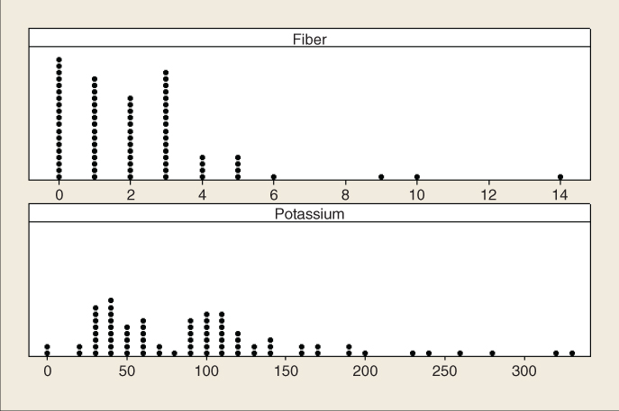
Figure 9.11 Fiber and potassium have different variabilities, thus requiring standardization before construction of user-defined composite.
We therefore proceed to perform the regression of nutritional rating on the following variables:
- Sugarsz
- Shelf 2

The results are provided in Table 9.13.
Table 9.13 Results from regression of rating on sugars, shelf 2, and the fiber/potassium composite
 |
Note first that the multicollinearity problem seems to have been resolved, with the VIF values all near 1. Note also, however, that the regression results are rather disappointing, with the values of ![]() , and s all underperforming the model results found in Table 9.8, from the model,
, and s all underperforming the model results found in Table 9.8, from the model, ![]() , which did not even include the potassium variable.
, which did not even include the potassium variable.
What is going on here? The problem stems from the fact that the fiber variable is a very good predictor of nutritional rating, especially when coupled with sugar content, as we shall see later on when we perform best subsets regression. Therefore, using the fiber variable to form a composite with a variable that has weaker correlation with rating dilutes the strength of fiber's strong association with rating, and so degrades the efficacy of the model.
Thus, reluctantly, we put aside this model (![]() ). One possible alternative is to change the weights in the composite, to increase the weight of fiber with respect to potassium. For example, we could use
). One possible alternative is to change the weights in the composite, to increase the weight of fiber with respect to potassium. For example, we could use ![]() . However, the model performance would still be slightly below that of using fiber alone. Instead, the analyst may be better advised to pursue principal components.
. However, the model performance would still be slightly below that of using fiber alone. Instead, the analyst may be better advised to pursue principal components.
Now, depending on the task confronting the analyst, multicollinearity may not in fact present a fatal defect. Weiss10 notes that multicollinearity “does not adversely affect the ability of the sample regression equation to predict the response variable.” He adds that multicollinearity does not significantly affect point estimates of the target variable, confidence intervals for the mean response value, or prediction intervals for a randomly selected response value. However, the data miner must therefore strictly limit the use of a multicollinear model to estimation and prediction of the target variable. Interpretation of the model would not be appropriate, because the individual coefficients may not make sense, in the presence of multicollinearity.
9.8 Variable Selection Methods
To assist the data analyst in determining which variables should be included in a multiple regression model, several different variable selection methods have been developed, including
- forward selection;
- backward elimination;
- stepwise selection;
- best subsets.
These variable selection methods are essentially algorithms to help construct the model with the optimal set of predictors.
9.8.1 The Partial F-Test
In order to discuss variable selection methods, we first need to learn about the partial F-test. Suppose that we already have p variables in the model, ![]() , and we are interested in whether one extra variable
, and we are interested in whether one extra variable ![]() should be included in the model or not. Recall earlier where we discussed the sequential sums of squares. Here, we would calculate the extra (sequential) sum of squares from adding
should be included in the model or not. Recall earlier where we discussed the sequential sums of squares. Here, we would calculate the extra (sequential) sum of squares from adding ![]() to the model, given that
to the model, given that ![]() are already in the model. Denote this quantity by
are already in the model. Denote this quantity by ![]() . Now, this extra sum of squares is computed by finding the regression sum of squares for the full model (including
. Now, this extra sum of squares is computed by finding the regression sum of squares for the full model (including ![]() and
and ![]() ), denoted
), denoted ![]() , and subtracting the regression sum of squares from the reduced model (including only
, and subtracting the regression sum of squares from the reduced model (including only ![]() ), denoted
), denoted ![]() . In other words:
. In other words:
that is,
The null hypothesis for the partial F-test is as follows:
- H0: No, the
 associated with
  does not contribute significantly to the regression sum of squares for a model already containing
  . Therefore, do not include
  in the model.
The alternative hypothesis is:
- Ha: Yes, the
 associated with
  does contribute significantly to the regression sum of squares for a model already containing
  . Therefore, do include
  in the model.
The test statistic for the partial F-test is the following:
where ![]() denotes the mean square error term from the full model, including
denotes the mean square error term from the full model, including ![]() and
and ![]() . This is known as the partial F-statistic for
. This is known as the partial F-statistic for ![]() . When the null hypothesis is true, this test statistic follows an
. When the null hypothesis is true, this test statistic follows an ![]() distribution. We would therefore reject the null hypothesis when
distribution. We would therefore reject the null hypothesis when ![]() is large, or when its associated p-value is small.
is large, or when its associated p-value is small.
An alternative to the partial F-test is the t-test. Now, an F-test with 1 and ![]() degrees of freedom is equivalent to a t-test with
degrees of freedom is equivalent to a t-test with ![]() degrees of freedom. This is due to the distributional relationship that
degrees of freedom. This is due to the distributional relationship that ![]() . Thus, either the F-test or the t-test may be performed. Similarly to our treatment of the t-test earlier in the chapter, the hypotheses are given by
. Thus, either the F-test or the t-test may be performed. Similarly to our treatment of the t-test earlier in the chapter, the hypotheses are given by
The associated models are
Under the null hypothesis, the test statistic ![]() follows a t distribution with
follows a t distribution with ![]() degrees of freedom. Reject the null hypothesis when the two-tailed p-value,
degrees of freedom. Reject the null hypothesis when the two-tailed p-value, ![]() , is small.
, is small.
Finally, we need to discuss the difference between sequential sums of squares, and partial sums of squares. The sequential sums of squares are as described earlier in the chapter. As each variable is entered into the model, the sequential sum of squares represents the additional unique variability in the response explained by that variable, after the variability accounted for by variables entered earlier in the model has been extracted. That is, the ordering of the entry of the variables into the model is germane to the sequential sums of squares.
However, ordering is not relevant to the partial sums of squares. For a particular variable, the partial sum of squares represents the additional unique variability in the response explained by that variable, after the variability accounted for by all the other variables in the model has been extracted. Table 9.14 shows the difference between sequential and partial sums of squares, for a model with four predictors, ![]() .
.
Table 9.14 The difference between sequential SS and partial SS
| Variable | Sequential SS | Partial SS |
9.8.2 The Forward Selection Procedure
The forward selection procedure starts with no variables in the model.
- Step 1. For the first variable to enter the model, select the predictor most highly correlated with the target. (Without loss of generality, denote this variable
 .) If the resulting model is not significant, then stop and report that no variables are important predictors; otherwise, proceed to step 2. Note that the analyst may choose the level of
  ; lower values make it more difficult to enter the model. A common choice is
  , but this is not set in stone.
 - Step 2. For each remaining variable, compute the sequential F-statistic for that variable, given the variables already in the model. For example, in this first pass through the algorithm, these sequential F-statistics would be
 ,
,  , and
, and  . On the second pass through the algorithm, these might be
  and
and  . Select the variable with the largest sequential F-statistic.
 - Step 3. For the variable selected in step 2, test for the significance of the sequential F-statistic. If the resulting model is not significant, then stop, and report the current model without adding the variable from step 2. Otherwise, add the variable from step 2 into the model and return to step 2.
9.8.3 The Backward Elimination Procedure
The backward elimination procedure begins with all the variables, or all of a user-specified set of variables, in the model.
- Step 1. Perform the regression on the full model; that is, using all available variables. For example, perhaps the full model has four variables,
 .
. - Step 2. For each variable in the current model, compute the partial F-statistic. In the first pass through the algorithm, these would be
 ,
,  ,
,  , and
, and  . Select the variable with the smallest partial F-statistic. Denote this value
  .
. - Step 3. Test for the significance of
 . If
. If  is not significant, then remove the variable associated with
  from the model, and return to step 2. If
  is significant, then stop the algorithm and report the current model. If this is the first pass through the algorithm, then the current model is the full model. If this is not the first pass, then the current model has been reduced by one or more variables from the full model. Note that the analyst may choose the level of
  needed to remove variables. Lower values make it more difficult to keep variables in the model.
9.8.4 The Stepwise Procedure
The stepwise procedure represents a modification of the forward selection procedure. A variable that has been entered into the model early in the forward selection process may turn out to be nonsignificant, once other variables have been entered into the model. The stepwise procedure checks on this possibility, by performing at each step a partial F-test, using the partial sum of squares, for each variable currently in the model. If there is a variable in the model that is no longer significant, then the variable with the smallest partial F-statistic is removed from the model. The procedure terminates when no further variables can be entered or removed. The analyst may choose both the level of ![]() required to enter the model, and the level of
required to enter the model, and the level of ![]() needed to remove variables, with
needed to remove variables, with ![]() chosen to be somewhat large than
chosen to be somewhat large than ![]() .
.
9.8.5 The Best Subsets Procedure
For data sets where the number of predictors is not too large, the best subsets procedure represents an attractive variable selection method. However, if there are more than 30 or so predictors, then the best subsets method encounters a combinatorial explosion, and becomes intractably slow.
The best subsets procedure works as follows:
- Step 1. The analyst specifies how many (k) models of each size he or she would like reported, as well as the maximum number of predictors (p) the analyst wants in the model.
- Step 2. All models of one predictor are built. Their
 , Mallows' Cp (see below), and s values are calculated. The best k models are reported, based on these measures.
 - Step 3. Then all models of two predictors are built. Their
 , Mallows' Cp, and s values are calculated, and the best k models are reported.
 - The procedure continues in this way until the maximum number of predictors (p) is reached. The analyst then has a listing of the best models of each size, 1, 2, …, p, to assist in the selection of the best overall model.
9.8.6 The All-Possible-Subsets Procedure
The four methods of model selection we have discussed are essentially optimization algorithms over a large sample space. Because of that, there is no guarantee that the globally optimal model will be found; that is, there is no guarantee that these variable selection algorithms will uncover the model with the lowest s, the highest ![]() , and so on (Draper and Smith11; Kleinbaum, Kupper, Nizam, and Muller12). The only way to ensure that the absolute best model has been found is simply to perform all the possible regressions. Unfortunately, in data mining applications, there are usually so many candidate predictor variables available that this method is simply not practicable. Not counting the null model
, and so on (Draper and Smith11; Kleinbaum, Kupper, Nizam, and Muller12). The only way to ensure that the absolute best model has been found is simply to perform all the possible regressions. Unfortunately, in data mining applications, there are usually so many candidate predictor variables available that this method is simply not practicable. Not counting the null model ![]() , there are
, there are ![]() possible models to be built, using p predictors.
possible models to be built, using p predictors.
For small numbers of predictors, it is not a problem to construct all possible regressions. For example, for ![]() predictors, there are
predictors, there are ![]() possible models. However, as the number of predictors starts to grow, the search space grows exponentially. For instance, for
possible models. However, as the number of predictors starts to grow, the search space grows exponentially. For instance, for ![]() predictors, there are
predictors, there are ![]() possible models, while for
possible models, while for ![]() predictors, there are
predictors, there are ![]() possible models. Thus, for most data mining applications, in which there may be hundreds of predictors, the all-possible-regressions procedure is not applicable. Therefore, the data miner may be inclined to turn to one of the four variable selection procedures discussed above. Even though there is no guarantee that the globally best model is found, these methods usually provide a useful set of models, which can provide positive results. The analyst can then adopt these models as starting points, and apply tweaks and modifications to coax the best available performance out of them.
possible models. Thus, for most data mining applications, in which there may be hundreds of predictors, the all-possible-regressions procedure is not applicable. Therefore, the data miner may be inclined to turn to one of the four variable selection procedures discussed above. Even though there is no guarantee that the globally best model is found, these methods usually provide a useful set of models, which can provide positive results. The analyst can then adopt these models as starting points, and apply tweaks and modifications to coax the best available performance out of them.
9.9 Gas Mileage Data Set
At this point, it may be helpful to turn to a new data set to illustrate the nuts and bolts of variable selection methods. We shall use the Gas Mileage data set,13 where the target variable MPG (miles per gallon) is estimated using four predictors: cab space, horsepower, top speed, and weight. Let us explore this data set a bit. Figure 9.12 shows scatter plots of the target MPG with each of the predictors. The relationship between MPG and horsepower does not appear to be linear. Using the bulging rule

Figure 9.12 Scatter plots of MPG with each predictor. Some non-linearity.
from Chapter 8, we therefore take the ln of each variable. The resulting scatter plots, shown in Figure 9.13, show improved linearity. We therefore proceed to perform linear regression of ln MPG on cab space, ln HP, top speed, and weight.
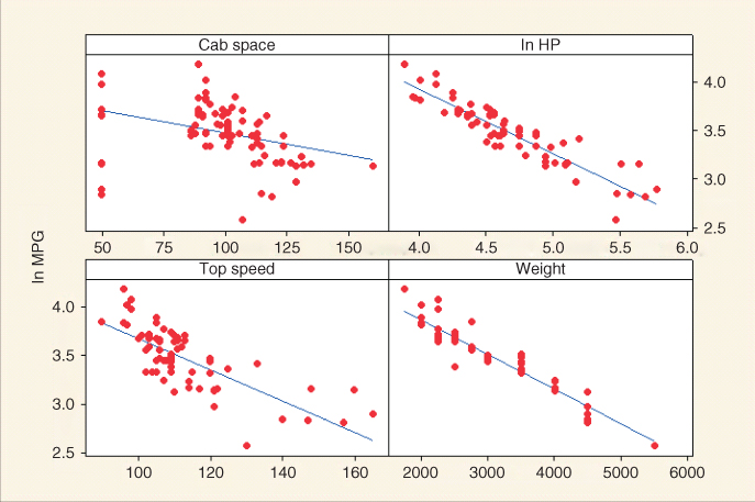
Figure 9.13 Scatter plots of ln MPG with each predictor (including ln HP). Improved linearity.
9.10 An Application of Variable Selection Methods
We would like the most parsimonious model that does not leave out any significant predictors. We shall apply the variable selection methods described above. We select the following commonly used thresholds of significance for variables entering and leaving the model: ![]() and
and ![]() .
.
9.10.1 Forward Selection Procedure Applied to the Gas Mileage Data Set
Table 9.15 shows the results for the forward selection method. We begin with no variables in the model. Then the variable most strongly correlated with ln MPG is selected, and, if significant, entered into the model. This variable is weight, which has the highest correlation with ln MPG, among the predictors. This is shown in the upper left of Table 9.15, showing weight as the first variable entered.
Table 9.15 Forward selection results
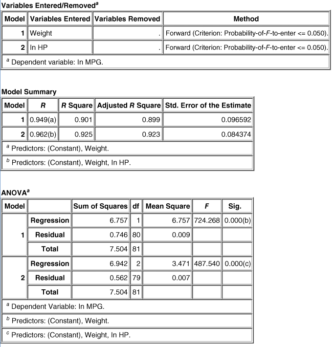 |
Then the sequential F-tests are performed, such as ![]() , and so on. It turns out that the highest sequential F-statistic is given by the significance test of
, and so on. It turns out that the highest sequential F-statistic is given by the significance test of ![]() , so that the variable ln HP becomes the second variable entered into the model, as shown in Table 9.15. Once again, the sequential F-tests are performed, but no further significant variables were found. Thus, the forward selection method prefers the following model:
, so that the variable ln HP becomes the second variable entered into the model, as shown in Table 9.15. Once again, the sequential F-tests are performed, but no further significant variables were found. Thus, the forward selection method prefers the following model:
Table 9.15 contains the ANOVA tables for the two models selected by the forward selection procedure. We may use these ANOVA results to calculate the sequential F-statistics. Model 1 represents the model with weight as the only predictor. Model 2 represents the model with both weight and ln HP entered as predictors.
As ![]() , we have
, we have
From Table 9.15, we have
 , and
, and , giving us:
The test statistic for the partial (or, in this case, sequential) F-test is the following:
From Table 9.15, we have
 , giving us:
With a sample size of 82, and p = 2 parameters in the model, this test statistic follows an ![]() distribution. The p-value for this test statistic is approximately zero, thereby rejecting the null hypothesis that fiber should not be included after sugars.
distribution. The p-value for this test statistic is approximately zero, thereby rejecting the null hypothesis that fiber should not be included after sugars.
9.10.2 Backward Elimination Procedure Applied to the Gas Mileage Data Set
In the backward elimination procedure, we begin with all of the variables in the model. The partial F-statistic is then calculated for each variable in the model (e.g., ![]() . The variable with the smallest partial F-statistic,
. The variable with the smallest partial F-statistic, ![]() , is examined, which in this case is cab space. If
, is examined, which in this case is cab space. If ![]() is not significant, which is the case here, then the variable is dropped from the model. Cab space is the first variable to be removed, as is shown in Table 9.16. On the next pass, the variable with the smallest partial F-statistic is top speed, which again is not significant. Thus, top speed becomes the second variable omitted from the model. No other variables are removed from the model, so that the backward elimination method prefers the same model as the forward selection method.
is not significant, which is the case here, then the variable is dropped from the model. Cab space is the first variable to be removed, as is shown in Table 9.16. On the next pass, the variable with the smallest partial F-statistic is top speed, which again is not significant. Thus, top speed becomes the second variable omitted from the model. No other variables are removed from the model, so that the backward elimination method prefers the same model as the forward selection method.
Table 9.16 Backward elimination results
 |
9.10.3 The Stepwise Selection Procedure Applied to the Gas Mileage Data Set
The stepwise selection procedure is a modification of the forward selection procedure, where the algorithm checks at each step whether all variables currently in the model are still significant. In this example, each variable that had been entered remained significant when the other variables were also entered. Thus, for this example, the results were the same as for the forward selection procedure, with the same model summaries as shown in Table 9.15.
9.10.4 Best Subsets Procedure Applied to the Gas Mileage Data Set
Table 9.17 provides the results from Minitab's application of the best subsets procedure on the gas mileage data set. The predictor variable names are given on the upper right, formatted vertically. Each horizontal line in the table represents a separate model, with the “X”s shown under the predictors included in a particular model. The best subsets procedure reports the two best models with p = 1 predictor, the two best models with p = 2 models, and so on. Thus, the first model has only weight; the second model has only ln HP; the third model has ln HP and weight; the fourth model has top speed and weight; and so on.
Table 9.17 Best subsets results for Gas Mileage data set (“best” model highlighed)
 |
Four model selection criteria are reported for each model: ![]() , Mallows' Cp, and s.
, Mallows' Cp, and s.
9.10.5 Mallows' Cp Statistic
We now discuss the ![]() statistic, developed by C. L. Mallows14. Mallows'
statistic, developed by C. L. Mallows14. Mallows' ![]() statistic takes the form:
statistic takes the form:
where ![]() represents the number of predictors in the current (working) model,
represents the number of predictors in the current (working) model, ![]() represents the error sum of squares of the model with p predictors, and
represents the error sum of squares of the model with p predictors, and ![]() represents the MSE of the full model; that is, the model with all predictors entered.
represents the MSE of the full model; that is, the model with all predictors entered.
For a model that fits well, it can be shown15 that ![]() . Thus, we would expect the value of
. Thus, we would expect the value of ![]() for a well-fitting model to take a value not far from
for a well-fitting model to take a value not far from ![]() . However, models that show a considerable lack of fit will take values of
. However, models that show a considerable lack of fit will take values of ![]() above (and sometimes far above)
above (and sometimes far above) ![]() . The full model, with all variables entered, always has
. The full model, with all variables entered, always has ![]() , but is often not the best model.
, but is often not the best model.
It is useful to plot the value of Mallows' ![]() against the number of predictors, p. Figure 9.14 shows such a plot for the gas mileage data set regression. (To increase granularity, the model with
against the number of predictors, p. Figure 9.14 shows such a plot for the gas mileage data set regression. (To increase granularity, the model with ![]() is omitted.) One heuristic for choosing the best model is to select the model where the value of
is omitted.) One heuristic for choosing the best model is to select the model where the value of ![]() first approaches or crosses the line
first approaches or crosses the line ![]() , as p increases.
, as p increases.

Figure 9.14 A plot of Mallows'  against the number of predictors, p, can help select the best model.
Consider Figure 9.14. However, the general trend for the values of ![]() is to fall as p increases, as can be seen from Figure 9.15. As we reach
is to fall as p increases, as can be seen from Figure 9.15. As we reach ![]() , we have
, we have ![]() , which is approaching the line
, which is approaching the line ![]() . This represents the model chosen by the other three variable selection methods.
. This represents the model chosen by the other three variable selection methods.
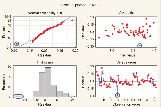
Figure 9.15 Normal probability plot shows skewness.
Finally, when we reach ![]() , we have, for one of the models,
, we have, for one of the models, ![]() , which is below the line
, which is below the line ![]() . Therefore, the Mallows'
. Therefore, the Mallows' ![]() heuristic would be to select this model as the working model. This model contains ln HP, top speed, and weight as predictors.
heuristic would be to select this model as the working model. This model contains ln HP, top speed, and weight as predictors.
Thus, we have two candidate working models:

Model A is supported by forward selection, backward elimination, and stepwise, and was nearly favored by best subsets. Model B is preferred by best subsets, but barely. Let us mention that one need not report only one model as a final model. Two or three models may be carried forward, and input sought from managers about which model may be most ameliorative of the business or research problem. However, it is often convenient to have one “working model” selected, because of the complexity of model building in the multivariate environment. However, recall the principal of parsimony, which states All things being equal, choose the simpler model. Because of parsimony, and because Model A did so well with most of the variable selection methods, it is recommended that we consider Model A to be our working model. The regression results for Model A are shown in Table 9.18.
Table 9.18 Regression results for model chosen by variable selection criteria
 |
Checking for the regression assumptions, each of the graphs in Figure 9.16 shows an outlier, the Subaru Loyale, which got lower gas mileage than expected, given its predictor values. Table 9.19 shows the regression results when this outlier is omitted. The precision of the regression is improved; for example, the standard error of the estimate, s, has decreased by 6.6%.
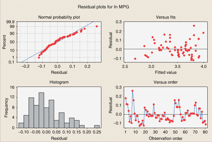
Figure 9.16 Outlier uncovered.
Table 9.19 Regression results improved a bit with outlier removed
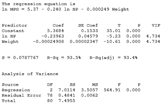 |
Figure 9.17 shows the plots for validation of the regression assumptions. With some slight right-skewness in the residuals, and some curvature in the residuals versus fitted values, these are not as tight as we might wish; in the exercises, we will try to deal with these issues. However, we are on the whole satisfied that our regression model provides a decent summary of the linear relationship between ln MPG and the predictors. Nevertheless, there still remains the problem of moderate multicollinearity, as shown by the VIF values close to 5 for the predictors. Thus, we now turn to a method made to deal with multicollinearity: principal components analysis.
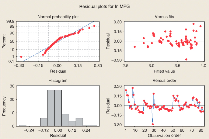
Figure 9.17 Regression assumptions.
9.11 Using the Principal Components as Predictors in Multiple Regression
Principal components16 may be used as predictors in a multiple regression model. Each record has a component value for each principal component, as shown in the rightmost four columns in Table 9.20. These component values may be used as predictors in a regression model, or, indeed, any analytical model.
Table 9.20 Each record has component weight values for each component
| Make/Model | MPG | ln HP | ln MPG | Cab Space_z | Horsepower_z | Top Speed_z | Weight_z | PrinComp1 | PrinComp2 | PrinComp3 | PrinComp4 |
| GM/GeoMetroXF1 | 65.400 | 3.892 | 4.181 | −0.442 | −1.199 | −1.169 | −1.648 | −0.770 | −0.246 | −1.454 | 2.449 |
| GM/GeoMetro | 56.000 | 4.007 | 4.025 | −0.307 | −1.093 | −1.098 | −1.341 | −0.805 | −0.167 | −1.081 | 1.896 |
| GM/GeoMetroLSI | 55.900 | 4.007 | 4.024 | −0.307 | −1.093 | −1.098 | −1.341 | −0.805 | −0.167 | −1.081 | 1.896 |
| SuzukiSwift | 49.000 | 4.248 | 3.892 | −0.307 | −0.829 | −0.528 | −1.341 | −0.173 | −0.081 | −1.518 | 0.115 |
| DaihatsuCharade | 46.500 | 3.970 | 3.839 | −0.307 | −1.128 | −1.169 | −1.341 | −0.885 | −0.177 | −1.026 | 2.094 |
| GM/GeoSprintTurbo | 46.200 | 4.248 | 3.833 | −0.442 | −0.829 | −0.528 | −1.341 | −0.199 | −0.229 | −1.450 | 0.079 |
| GM/GeoSprint | 45.400 | 4.007 | 3.816 | −0.307 | −1.093 | −1.098 | −1.341 | −0.805 | −0.167 | −1.081 | 1.896 |
| HondaCivicCRXHF | 59.200 | 4.127 | 4.081 | −2.202 | −0.970 | −1.027 | −1.034 | −1.229 | −2.307 | 0.302 | 1.012 |
| HondaCivicCRXHF | 53.300 | 4.127 | 3.976 | −2.202 | −0.970 | −1.027 | −1.034 | −1.229 | −2.307 | 0.302 | 1.012 |
| DaihatsuCharade | 43.400 | 4.382 | 3.770 | −0.217 | −0.653 | −0.386 | −1.034 | −0.118 | −0.039 | −1.189 | −0.246 |
| SubaruJusty | 41.100 | 4.290 | 3.716 | −0.442 | −0.776 | −0.671 | −1.034 | −0.473 | −0.328 | −0.860 | 0.686 |
| HondaCivicCRX | 40.900 | 4.522 | 3.711 | −2.202 | −0.442 | 0.042 | −1.034 | −0.027 | −2.145 | −0.528 | −1.953 |
First, the predictors from the original data set are all standardized, using z-scores. Then principal components analysis is performed on the standardized predictors, with varimax rotation. The variance-explained results are shown in Table 9.21. The varimax-rotated solution has nearly attained 100% of variance explained by three components. We therefore extract three components, to be used as predictors for our regression model.17
Table 9.21 Percentage of variance explained for the rotated solution for three components is nearly 100%
| Total Variance Explained | |||||||||
| Initial Eigenvalues | Extraction Sums of Squared Loadings | Rotation Sums of Squared Loadings | |||||||
| Component | Total | % of Variance | Cumulative % | Total | % of Variance | Cumulative % | Total | % of Variance | Cumulative % |
| 1 | 2.689 | 67.236 | 67.236 | 2.689 | 67.236 | 67.236 | 2.002 | 50.054 | 50.054 |
| 2 | 1.100 | 27.511 | 94.747 | 1.100 | 27.511 | 94.747 | 1.057 | 26.436 | 76.490 |
| 3 | 0.205 | 5.137 | 99.884 | 0.205 | 5.137 | 99.884 | 0.935 | 23.386 | 99.876 |
| 4 | 0.005 | 0.116 | 100.000 | 0.005 | 0.116 | 100.000 | 0.005 | 0.124 | 100.000 |
Extraction method: Principal component analysis.
Table 9.22 shows the unrotated and rotated component weights, with weights less than 0.5 hidden, for clarity. Brief component profiles for the rotated solution are as follows:
- Component 1: Muscle. This component combines top speed and horsepower.
- Component 2: Roominess. The only variable is cab space.
- Component 3: Weight. The only variable is weight.
Table 9.22 Component weights, for the unrotated and rotated solutions
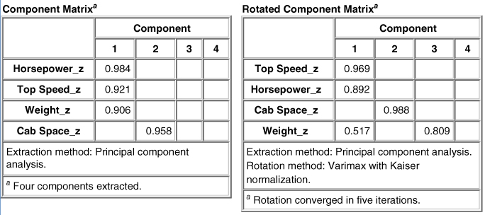 |
Regression of ln MPG on the three principal components is performed, with the results shown in Table 9.23 and the residual plots shown in Figure 9.15. Note that the multicollinearity problem has been solved, because the VIF statistics all equal a perfect 1.0. However, the normal probability plot of the residuals shows concave curvature, indicating right-skewness. We therefore apply the following Box–Cox transformation to MPG, to reduce the skewness:
The residual plots for the resulting regression of ![]() on the principal components are shown in Figure 9.18. The skewness has mostly been dealt with. These plots are not perfect. Specifically, there appears to be a systematic difference for the set of vehicles near the end of the data set in observation order. A glance at the data set indicates these are luxury cars, such as a Rolls–Royce and a Jaguar, which may follow a somewhat different gas mileage model. Overall, we find the plots indicate broad validation of the regression assumptions. Remember, in the world of dirty data, perfect validation of the assumptions may be elusive.
on the principal components are shown in Figure 9.18. The skewness has mostly been dealt with. These plots are not perfect. Specifically, there appears to be a systematic difference for the set of vehicles near the end of the data set in observation order. A glance at the data set indicates these are luxury cars, such as a Rolls–Royce and a Jaguar, which may follow a somewhat different gas mileage model. Overall, we find the plots indicate broad validation of the regression assumptions. Remember, in the world of dirty data, perfect validation of the assumptions may be elusive.
Table 9.23 Regression using principal components solves the multicollinearity problem
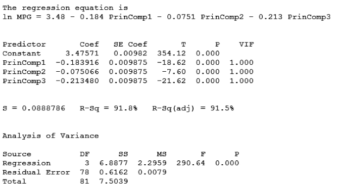 |

Figure 9.18 Observation order shows luxury cars may be different.
The regression results for regression of ![]() on the principal components are shown in Table 9.24. Note the following:
on the principal components are shown in Table 9.24. Note the following:
- Multicollinearity remains vanquished, with all VIF = 1.0.
 , not quite as good as the 93.5% for the model not accounting for multicollinearity.
- Note the group of last four unusual observations, all high leverage points, consists of a Mercedes, a Jaguar, a BMW, and a Rolls–Royce. The Rolls–Royce is the most extreme outlier.
Table 9.24 Regression of MPGBC 0.75 on the principal components
 |
In the exercises, we invite the analyst to further improve this model, either by tweaking the Box–Cox transformation, or through an indicator variable for the luxury cars, or some other means.
R References
- Harrell FE Jr. 2014. rms: Regression modeling strategies. R package version 4.1-3. http://CRAN.R-project.org/package=rms.
- Fox J, Weisberg S. An {R} Companion to Applied Regression. 2nd ed. Thousand Oaks, CA: Sage; 2011. http://socserv.socsci.mcmaster.ca/jfox/Books/Companion.
- Ligges U, Mächler M. Scatterplot3d – an R Package for visualizing multivariate data. Journal of Statistical Software 2003;8(11):1–20.
- R Core Team. R: A Language and Environment for Statistical Computing. Vienna, Austria: R Foundation for Statistical Computing; 2012. ISBN: 3-900051-07-0,http://www.R-project.org/.
- Revelle W. psych: Procedures for Personality and Psychological Research. Evanston, Illinois, USA: Northwestern University; 2013. . http://CRAN.R-project.org/package=psych Version=1.4.2.
- Thomas Lumley using Fortran code by Alan Miller. 2009. leaps: regression subset selection. R package version 2.9. http://CRAN.R-project.org/package=leaps.
- Venables WN, Ripley BD. Modern Applied Statistics with S. 4th ed. New York: Springer; 2002. ISBN: 0-387-95457-0.
Exercises
Clarifying The Concepts
1. Indicate whether the following statements are true or false. If the statement is false, alter it so that the statement becomes true.
- If we would like to approximate the relationship between a response and two continuous predictors, we would need a plane.
- In linear regression, while the response variable is typically continuous, it may be categorical as well.
- In general, for a multiple regression with m predictor variables, we would interpret coefficient
 as follows: “the estimated change in the response variable for a unit increase in variable
  is
is  .”
.” - In multiple regression, the residual is represented by the vertical distance between the data point and the regression plane or hyperplane.
- Whenever a new predictor variable is added to the model, the value of
 always goes up.
 - The alternative hypothesis in the F-test for the overall regression asserts that the regression coefficients all differ from zero.
- The standard error of the estimate is a valid measure of the usefulness of the regression, without reference to an inferential model (i.e., the assumptions need not be relevant).
- If we were to use only the categorical variables as predictors, then we would have to use analysis of variance and could not use linear regression.
- For use in regression, a categorical variable with k categories must be transformed into a set of k indicator variables.
- The first sequential sum of squares is exactly the value for SSR from the simple linear regression of the response on the first predictor.
- The VIF has a minimum of zero, but no upper limit.
- A variable that has been entered into the model early in the forward selection process will remain significant, once other variables have been entered into the model.
- The variable selection criteria for choosing the best model account for the multicollinearity among the predictors.
- The VIFs for principal components using varimax rotation always equal 1.0.
2. Clearly explain why s and ![]() are preferable to
are preferable to ![]() as measures for model building.
as measures for model building.
3. Explain the difference between the t-test and the F-test for assessing the significance of the predictors.
4. Construct indicator variables for the categorical variable class, which takes four values, freshman, sophomore, junior, and senior.
5. When using indicator variables, explain the meaning and interpretation of the indicator variable coefficients, graphically and numerically.
6. Discuss the concept of the level of significance ![]() . At what value should it be set? Who should decide the value of
. At what value should it be set? Who should decide the value of ![]() ? What if the observed p-value is close to
? What if the observed p-value is close to ![]() ? Describe a situation where a particular p-value will lead to two different conclusions, given two different values for
? Describe a situation where a particular p-value will lead to two different conclusions, given two different values for ![]() .
.
7. Explain what it means when ![]() is much less than
is much less than ![]() .
.
8. Explain the difference between the sequential sums of squares and the partial sums of squares. For which procedures do we need these statistics?
9. Explain some of the drawbacks of a set of predictors with high multicollinearity.
10. Which statistics report the presence of multicollinearity in a set of predictors? Explain, using the formula, how this statistic works. Also explain the effect that large and small values of this statistic will have on the standard error of the coefficient.
11. Compare and contrast the effects that multicollinearity has on the point and intervals estimates of the response versus the values of the predictor coefficients.
12. Describe the differences and similarities among the forward selection procedure, the backward elimination procedure, and the stepwise procedure.
13. Describe how the best subsets procedure works. Why not always use the best subsets procedure?
14. Describe the behavior of Mallows' ![]() statistic, including the heuristic for choosing the best model.
statistic, including the heuristic for choosing the best model.
15. Suppose we wished to limit the number of predictors in the regression model to a lesser number than those obtained using the default settings in the variable selection criteria. How should we alter each of the selection criteria? Now, suppose we wished to increase the number of predictors. How then should we alter each of the selection criteria?
16. Explain the circumstances under which the value for ![]() would reach 100%. Now explain how the p-value for any test statistic could reach zero.
would reach 100%. Now explain how the p-value for any test statistic could reach zero.
Working With The Data
For Exercises 17–27, consider the multiple regression output from SPSS in Table 9.25, using the nutrition data set, found on the book web site, www.DataMiningConsultant.com.
Table 9.25 Regression results for Exercises 17–27
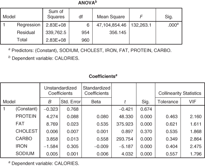 |
17. What is the response? What are the predictors?
18. What is the conclusion regarding the significance of the overall regression? How do you know? Does this mean that all of the predictors are important? Explain.
19. What is the typical error in prediction? (Hint: This may take a bit of digging.)
20. How many foods are included in the sample?
21. How are we to interpret the value of ![]() , the coefficient for the constant term? Is this coefficient significantly different from zero? Explain how this makes sense.
, the coefficient for the constant term? Is this coefficient significantly different from zero? Explain how this makes sense.
22. Which of the predictors probably does not belong in the model? Explain how you know this. What might be your next step after viewing these results?
23. Suppose we omit cholesterol from the model and rerun the regression. Explain what will happen to the value of ![]() .
.
24. Which predictor is negatively associated with the response? Explain how you know this.
25. Discuss the presence of multicollinearity. Evaluate the strength of evidence for the presence of multicollinearity. On the basis of this, should we turn to principal components analysis?
26. Clearly and completely express the interpretation for the coefficient for sodium.
27. Suppose a certain food was predicted to have 60 calories fewer than it actually has, based on its content of the predictor variables. Would this be considered unusual? Explain specifically how you would determine this.
For Exercises 28–29, next consider the multiple regression output from SPSS in Table 9.26. Three predictor variables have been added to the analysis in Exercises 17–27: saturated fat, monounsaturated fat, and polyunsaturated fat.
Table 9.26 Regression results for Exercises 28–29
| Coefficientsa | ||||||||
| Unstandardized coefficients | Standardized Coefficients | Collinearity Statistics | ||||||
| Model | B | Std. Error | Beta | t | Sig. | Tolerance | VIF | |
| 1 | (Constant) | −0.158 | 0.772 | −0.205 | 0.838 | |||
| PROTEIN | 4.278 | 0.088 | 0.080 | 48.359 | 0.000 | 0.457 | 2.191 | |
| FAT | 9.576 | 1.061 | 0.585 | 9.023 | 0.000 | 0.000 | 3379.867 | |
| CHOLEST | 1.539E−02 | 0.008 | 0.003 | 1.977 | 0.048 | 0.420 | 2.382 | |
| CARBO | 3.860 | 0.014 | 0.558 | 285.669 | 0.000 | 0.325 | 3.073 | |
| IRON | −1.672 | 0.314 | −0.010 | −5.328 | 0.000 | 0.377 | 2.649 | |
| SODIUM | 5.183E−03 | 0.001 | 0.006 | 3.992 | 0.000 | 0.555 | 1.803 | |
| SAT_FAT | −1.011 | 1.143 | −0.020 | −0.884 | 0.377 | 0.002 | 412.066 | |
| MONUNSAT | −0.974 | 1.106 | −0.025 | −0.881 | 0.379 | 0.002 | 660.375 | |
| POLUNSAT | −0.600 | 1.111 | −0.013 | −0.541 | 0.589 | 0.002 | 448.447 | |
a Dependent variable: CALORIES.
28. Evaluate the strength of evidence for the presence of multicollinearity.
29. On the basis of this, should we turn to principal components analysis?
For Exercises 30–37, consider the multiple regression output from SPSS in Table 9.27, using the New York data set, found on the book web site, www.DataMiningConsultant.com. The data set contains demographic information about a set of towns in New York state. The response “MALE_FEM” is the number of males in the town for every 100 females. The predictors are the percentage under the age of 18, the percentage between 18 and 64, and the percentage over 64 living in the town (all expressed in percents such as “57.0”), along with the town's total population.
Table 9.27 Regression results for Exercises 30–37
 |
30. Note that the variable PCT_O64 was excluded. Explain why this variable was automatically excluded from the analysis by the software. (Hint: Consider the analogous case of using too many indicator variables to define a particular categorical variable.)
31. What is the conclusion regarding the significance of the overall regression?
32. What is the typical error in prediction?
33. How many towns are included in the sample?
34. Which of the predictors probably does not belong in the model? Explain how you know this. What might be your next step after viewing these results?
35. Suppose we omit TOT_POP from the model and rerun the regression. Explain what will happen to the value of ![]() .
.
36. Discuss the presence of multicollinearity. Evaluate the strength of evidence for the presence of multicollinearity. On the basis of this, should we turn to principal components analysis?
37. Clearly and completely express the interpretation for the coefficient for PCT_U18. Discuss whether this makes sense.
Hands-On Analysis
For Exercises 38–41, use the nutrition data set, found on the book web site, www.DataMiningConsultant.com.
38. Build the best multiple regression model you can for the purposes of predicting calories, using all the other variables as the predictors. Do not worry about whether the predictor coefficients are stable or not. Compare and contrast the results from the forward selection, backward elimination, and stepwise variable selection procedures.
39. Apply the best subsets procedure, and compare against the previous methods.
40. (Extra credit). Write a script that will perform all possible regressions. Did the variable selection algorithms find the best regression?
41. Next, build the best multiple regression model you can for the purposes both of predicting the response and of profiling the predictors' individual relationship with the response. Make sure you account for multicollinearity.
For Exercises 42–44, use the New York data set, found on the book web site.
42. Build the best multiple regression model you can for the purposes of predicting the response, using the gender ratio as the response, and all the other variables as the predictors. Compare and contrast the results from the forward selection, backward elimination, and stepwise variable selection procedures.
43. Apply the best subsets procedure, and compare against the previous methods.
44. Perform all possible regressions. Did the variable selection algorithms find the best regression?
For Exercises 45–49, use the crash data set, found on the book web site.
45. Build the best multiple regression model you can for the purposes of predicting head injury severity, using all the other variables as the predictors.
46. Determine which variables must be made into indicator variables.
47. Determine which variables might be superfluous.
48. Build two parallel models, one where we account for multicollinearity, and another where we do not. For which purposes may each of these models be used?
49. Continuing with the crash data set, combine the four injury measurement variables into a single variable, defending your choice of combination function. Build the best multiple regression model you can for the purposes of predicting injury severity, using all the other variables as the predictors. Build two parallel models, one where we account for multicollinearity, and another where we do not. For which purposes may each of these models be used?
For Exercises 50–51, see if you can improve on the regression model of ln MPG on ln HP and weight.
50. Use a Box–Cox transformation to try to eliminate the skewness in the normal probability plot.
51. Do you see some curvature in the residuals versus fitted values plot? Produce a plot of the residuals against each of the predictors. Any curvature? Add a quadratic term of one of the predictors (e.g., ![]() ) to the model, and see if this helps.
) to the model, and see if this helps.
52. Using the four criteria from Chapter 5, determine the best number of principal components to extract for the gas mileage data.
53. Take a shot at improving the regression of ![]() on the principal components. For example, you may wish to tweak the Box–Cox transformation, or you may wish to use an indicator variable for the luxury cars. Using whatever means you can bring to bear, obtain your best model that deals with multicollinearity and validates the regression assumptions.
on the principal components. For example, you may wish to tweak the Box–Cox transformation, or you may wish to use an indicator variable for the luxury cars. Using whatever means you can bring to bear, obtain your best model that deals with multicollinearity and validates the regression assumptions.