2.1 Bayesian inference is reallocation of credibility across possibilities

Suppose we step outside one morning and notice that the sidewalk is wet, and wonder why. We consider all possible causes of the wetness, including possibilities such as recent rain, recent garden irrigation, a newly erupted underground spring, a broken sewage pipe, a passerby who spilled a drink, and so on. If all we know until this point is that some part of the sidewalk is wet, then all those possibilities will have some prior credibility based on previous knowledge. For example, recent rain may have greater prior probability than a spilled drink from a passerby. Continuing on our outside journey, we look around and collect new observations. If we observe that the sidewalk is wet for as far as we can see, as are the trees and parked cars, then we re-allocate credibility to the hypothetical cause of recent rain. The other possible causes, such as a passerby spilling a drink, would not account for the new observations. On the other hand, if instead we observed that the wetness was localized to a small area, and there was an empty drink cup a few feet away, then we would re-allocate credibility to the spilled-drink hypothesis, even though it had relatively low prior probability. This sort of reallocation of credibility across possibilities is the essence of Bayesian inference.

Another example of Bayesian inference has been immortalized in the words of the fictional detective Sherlock Holmes, who often said to his sidekick, Doctor Watson: “How often have I said to you that when you have eliminated the impossible, whatever remains, however improbable, must be the truth?” (Doyle, 1890, chap. 6) Although this reasoning was not described by Holmes or Watson or Doyle as Bayesian inference, it is. Holmes conceived of a set of possible causes for a crime. Some of the possibilities may have seemed very improbable, a priori. Holmes systematically gathered evidence that ruled out a number of the possible causes. If all possible causes but one were eliminated, then (Bayesian) reasoning forced him to conclude that the remaining possible cause was fully credible, even if it seemed improbable at the start.

Figure 2.1 illustrates Holmes' reasoning. For the purposes of illustration, we suppose that there are just four possible causes of the outcome to be explained. We label the causes A, B, C, and D. The heights of the bars in the graphs indicate the credibility of the candidate causes. (“Credibility” is synonymous with “probability”; here I use the everyday term “credibility” but later in the book, when mathematical formalisms are introduced, I will also use the term “probability.”) Credibility can range from zero to one. If the credibility of a candidate cause is zero, then the cause is definitely not responsible. If the credibility of a candidate cause is one, then the cause definitely is responsible. Because we assume that the candidate causes are mutually exclusive and exhaust all possible causes, the total credibility across causes sums to one.

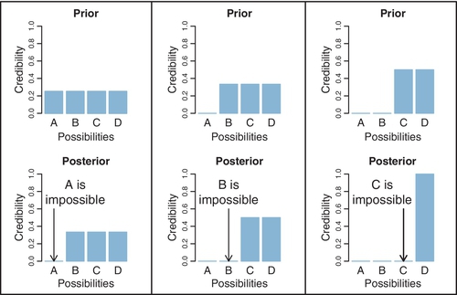
The upper-left panel of Figure 2.1 shows that the prior credibilities of the four candidate causes are equal, all at 0.25. Unlike the case of the wet sidewalk, in which prior knowledge suggested that rain may be a more likely cause than a newly erupted underground spring, the present illustration assumes equal prior credibilities of the candidate causes. Suppose we make new observations that rule out candidate cause A. For example, if A is a suspect in a crime, we may learn that A was far from the crime scene at the time. Therefore, we must re-allocate credibility to the remaining candidate causes, B through D, as shown in the lower-left panel of Figure 2.1. The re-allocated distribution of credibility is called the posterior distribution because it is what we believe after taking into account the new observations. The posterior distribution gives zero credibility to cause A, and allocates credibilities of 0.33 (i.e., 1/3) to candidate causes B, C, and D.

The posterior distribution then becomes the prior beliefs for subsequent observations. Thus, the prior distribution in the upper-middle of Figure 2.1 is the posterior distribution from the lower left. Suppose now that additional new evidence rules out candidate cause B. We now must re-allocate credibility to the remaining candidate causes, C and D, as shown in the lower-middle panel of Figure 2.1. This posterior distribution becomes the prior distribution for subsequent data collection, as shown in the upper-right panel of Figure 2.1. Finally, if new data rule out candidate cause C, then all credibility must fall on the remaining cause, D, as shown in the lower-right panel of Figure 2.1, just as Holmes declared. This reallocation of credibility is not only intuitive, it is also what the exact mathematics of Bayesian inference prescribe, as will be explained later in the book.

The complementary form of reasoning is also Bayesian, and can be called judicial exoneration. Suppose there are several possible culprits for a crime, and that these suspects are mutually unaffiliated and exhaust all possibilities. If evidence accrues that one suspect is definitely culpable, then the other suspects are exonerated.

This form of exoneration is illustrated in Figure 2.2. The upper panel assumes that there are four possible causes for an outcome, labeled A, B, C, and D. We assume that the causes are mutually exclusive and exhaust all possibilities. In the context of suspects for a crime, the credibility of the hypothesis that suspect A committed the crime is the culpability of the suspect. So it might be easier in this context to think of culpability instead of credibility. The prior culpabilities of the four suspects are, for this illustration, set to be equal, so the four bars in the upper panel of Figure 2.2 are all of height 0.25. Suppose that new evidence firmly implicates suspect D as the culprit. Because the other suspects are known to be unaffiliated, they are exonerated, as shown in the lower panel of Figure 2.2. As in the situation of Holmesian deduction, this exoneration is not only intuitive, it is also what the exact mathematics of Bayesian inference prescribe, as will be explained later in the book.

2.1.1 Data are noisy and inferences are probabilistic

The cases of Figures 2.1 and 2.2 assumed that observed data had definitive, deterministic relations to the candidate causes. For example, the fictional Sherlock Holmes may have found a footprint at the scene of the crime and identified the size and type of shoe with complete certainty, thereby completely ruling out or implicating a particular candidate suspect. In reality, of course, data have only probabilistic relations to their underlying causes. A real detective might carefully measure the footprint and the details of its tread, but these measurements would only probabilistically narrow down the range of possible shoes that might have produced the print. The measurements are not perfect, and the footprint is only an imperfect representation of the shoe that produced it. The relation between the cause (i.e., the shoe) and the measured effect (i.e., the footprint) is full of random variation.

In scientific research, measurements are replete with randomness. Extraneous influences contaminate the measurements despite tremendous efforts to limit their intrusion. For example, suppose we are interested in testing whether a new drug reduces blood pressure in humans. We randomly assign some people to a test group that takes the drug, and we randomly assign some other people to a control group that takes a placebo. The procedure is “double blind” so that neither the participants nor the administrators know which person received the drug or the placebo (because that information is indicated by a randomly assigned code that is decrypted after the data are collected). We measure the participants' blood pressures at set times each day for several days. As you can imagine, blood pressures for any single person can vary wildly depending on many influences, such as exercise, stress, recently eaten foods, etc. The measurement of blood pressure is itself an uncertain process, as it depends on detecting the sound of blood flow under a pressurized sleeve. Blood pressures are also very different from one person to the next. The resulting data, therefore, are extremely messy, with tremendous variability within each group, and tremendous overlap across groups. Thus, there will be many measured blood pressures in the drug group that are higher than blood pressures in the placebo group, and vice versa. From these two dispersed and overlapping heaps of numbers, we want to infer how big a difference there is between the groups, and how certain we can be about that difference. The problem is that for any particular real difference between the drug and the placebo, its measurable effect is only a random impression.

All scientific data have some degree of “noise” in their values. The techniques of data analysis are designed to infer underlying trends from noisy data. Unlike Sherlock Holmes, who could make an observation and completely rule out some possible causes, we can collect data and only incrementally adjust the credibility of some possible trends. We will see many realistic examples later in the book. The beauty of Bayesian analysis is that the mathematics reveal exactly how much to re-allocate credibility in realistic probabilistic situations.

Here is a simplified illustration of Bayesian inference when data are noisy. Suppose there is a manufacturer of inflated bouncy balls, and the balls are produced in four discrete sizes, namely diameters of 1.0, 2.0, 3.0, and 4.0 (on some scale of distance such as decimeters). The manufacturing process is quite variable, however, because of randomness in degrees of inflation even for a single size ball. Thus, balls of manufactured size 3 might have diameters of 1.8 or 4.2, even though their average diameter is 3.0. Suppose we submit an order to the factory for three balls of size 2. We receive three balls and measure their diameters as best we can, and find that the three balls have diameters of 1.77, 2.23, and 2.70. From those measurements, can we conclude that the factory correctly sent us three balls of size 2, or did the factory send size 3 or size 1 by mistake, or even size 4?

Figure 2.3 shows a Bayesian answer to this question. The upper graph shows the four possible sizes, with blue bars at positions 1, 2, 3, and 4. The prior credibilities of the four sizes are set equal, at heights of 0.25, representing the idea that the factory received the order for three balls, but may have completely lost track of which size was ordered, hence any size is equally possible to have been sent.

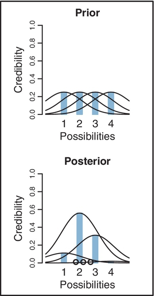
At this point, we must specify the form of random variability in ball diameters. For purposes of illustration, we will suppose that ball diameters are centered on their manufactured size, but could be bigger or smaller depending on the amount of inflation. The bell-shaped curves in Figure 2.3 indicate the probability of diameters produced by each size. Thus, the bell-shaped curve centered on size 2 indicates that size-2 balls are usually about 2.0 units in diameter, but could be much bigger or smaller because of randomness in inflation. The horizontal axis in Figure 2.3 is playing double duty as a scale for the ball sizes (i.e., blue bars) and for the measured diameters (suggested by the bell-shaped distributions).

The lower panel of Figure 2.3 shows the three measured diameters plotted as circles on the horizontal axis. You can see that the measured diameters are closest to sizes 2 or 3, but the bell-shaped distributions reveal that even size 1 could sometimes produce balls of those diameters. Intuitively, therefore, we would say that size 2 is most credible, given the data, but size 3 is also somewhat possible, and size 1 is remotely possible, but size 4 is rather unlikely. These intuitions are precisely reflected by Bayesian analysis, which is shown in the lower panel of Figure 2.3. The heights of the blue bars show the exact reallocation of credibility across the four candidate sizes. Given the data, there is 56% probability that the balls are size 2, 31% probability that the balls are size 3, 11% probability that the balls are size 1, and only 2% probability that the balls are size 4.

Inferring the underlying manufactured size of the balls from their “noisy” individual diameters is analogous to data analysis in real-world scientific research and applications. The data are noisy indicators of the underlying generator. We hypothesize a range of possible underlying generators, and from the data we infer their relative credibilities.

As another example, consider testing people for illicit drug use. A person is taken at random from a population and given a blood test for an illegal drug. From the result of the test, we infer whether or not the person has used the drug. But, crucially, the test is not perfect, it is noisy. The test has a non-trivial probability of producing false positives and false negatives. And we must also take into account our prior knowledge that the drug is used by only a small proportion of the population. Thus, the set of possibilities has two values: The person uses the drug or does not. The two possibilities have prior credibilities based on previous knowledge of how prevalent drug use is in the population. The noisy datum is the result of the drug test. We then use Bayesian inference to re-allocate credibility across the possibilities. As we will see quantitatively later in the book, the posterior probability of drug use is often surprisingly small even when the test result is positive, because the prior probability of drug use is small and the test is noisy. This is true not only for tests of drug use, but also for tests of diseases such as cancer. A related real-world application of Bayesian inference is detection of spam in email. Automated spam filters often use Bayesian inference to compute a posterior probability that an incoming message is spam.

In summary, the essence of Bayesian inference is reallocation of credibility across possibilities. The distribution of credibility initially reflects prior knowledge about the possibilities, which can be quite vague. Then new data are observed, and the credibility is re-allocated. Possibilities that are consistent with the data garner more credibility, while possibilities that are not consistent with the data lose credibility. Bayesian analysis is the mathematics of re-allocating credibility in a logically coherent and precise way.

2.2 Possibilities are parameter values in descriptive models

A key step in Bayesian analysis is defining the set of possibilities over which credibility is allocated. This is not a trivial step, because there might always be possibilities beyond the ones we include in the initial set. (For example, the wetness on the sidewalk might have been caused by space aliens who were crying big tears.) But we get the process going by choosing a set of possibilities that covers a range in which we are interested. After the analysis, we can examine whether the data are well described by the most credible possibilities in the considered set. If the data seem not to be well described, then we can consider expanding the set of possibilities. This process is called a posterior predictive check and will be explained later in the book.

Consider again the example of the blood-pressure drug, in which blood pressures are measured in one group that took the drug and in another group that took a placebo. We want to know how much difference there is in the tendencies of the two groups: How big is the difference between the typical blood pressure in one group versus the typical blood pressure in the other group, and how certain can we be of the difference? The magnitude of difference describes the data, and our goal is to assess which possible descriptions are more or less credible.

In general, data analysis begins with a family of candidate descriptions for the data. The descriptions are mathematical formulas that characterize the trends and spreads in the data. The formulas themselves have numbers, called parameter values, that determine the exact shape of mathematical forms. You can think of parameters as control knobs onmathematical devices that simulate data generation. If you change the value of a parameter, it changes a trend in the simulated data, just like if you change the volume control on a music player, it changes the intensity of the sound coming out of the player.

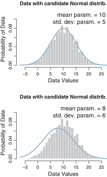
In previous studies of statistics or mathematics, you may have encountered the so-called normal distribution, which is a bell-shaped distribution often used to describe data. It was alluded to above in the example of the inflated bouncy balls (see Figure 2.3). The normal distribution has two parameters, called the mean and standard deviation. The mean is a control knob in the mathematical formula for the normal distribution that controls the location of the distribution's central tendency. The mean is sometimes called a location parameter. The standard deviation is another control knob in the mathematical formula for the normal distribution that controls the width or dispersion of the distribution. The standard deviation is sometimes called a scale parameter. The mathematical formula for the normal distribution converts the parameter values to a particular bell-like shape for the probabilities of data values.

Figure 2.4 shows some data with candidate normal distributions superimposed. The data are shown as a histogram, which plots vertical bars that have heights indicating how much of the data falls within the small range spanned by the bar. The histogram appears to be roughly unimodal and left-right symmetric. The upper panel superimposes a candidate description of the data in the form of a normal distribution that has a mean of 10 and a standard deviation of 5. This choice of parameter values appears to describe the data well. The lower panel shows another choice of parameter values, with a mean of 8 and a standard deviation of 6. While this candidate description appears to be plausible, it is not as good as the upper panel. The role of Bayesian inference is to compute the exact relative credibilities of candidate parameter values, while also taking into account their prior probabilities.

In realistic applications, the candidate parameter values can form an infinite continuum, not only a few discrete options. The location parameter of the normal distribution can take on any value from negative to positive infinity. Bayesian inference operates without trouble on infinite continuums.

There are two main desiderata for a mathematical description of data. First, the mathematical form should be comprehensible with meaningful parameters. Just as it would be fruitless to describe the data in a language that we do not know, it would be fruitless to describe the data with a mathematical form that we do not understand, with parameters that we cannot interpret. In the case of a normal distribution, for example, the mean parameter and standard-deviation parameter are directly meaningful as the location and scale of the distribution. Throughout this book, we will use mathematical descriptions that have meaningful parameters. Thus, Bayesian analysis reallocates credibility among parameter values within a meaningful space of possibilities defined by the chosen model.

The second desideratum for a mathematical description is that it should be descriptively adequate, which means, loosely, that the mathematical form should “look like” the data. There should not be any important systematic discrepancies between trends in the data and the form of the model. Deciding whether or not an apparent discrepancy is important or systematic is not a definite process. In early stages of research, we might be satisfied with a rough, “good enough” description of data, because it captures meaningful trends that are interesting and novel relative to previous knowledge. As the field of research matures, we might demand more and more accurate descriptions of data. Bayesian analysis is very useful for assessing the relative credibility of different candidate descriptions of data.

It is also important to understand that mathematical descriptions of data are not necessarily causal explanations of data. To say that the data in Figure 2.4 are well described by a normal distribution with mean of 10 and standard deviation of 5 does not explain what process caused the data to have that form. The parameters are “meaningful” only in the context of the familiar mathematical form defined by the normal distribution; the parameter values have no necessary meaning with respect to causes in the world. In some applications, the mathematical model might be motivated as a description of a natural process that generated the data, and thereby the parameters and mathematical form can refer to posited states and processes in the world. For example, in the case of the inflated bouncy balls (Figure 2.3), the candidate parameter values were interpreted as “sizes” at the manufacturer, and the underlying size, combined with random inflation, caused the observed data value. But reference to physical states or processes is not necessary for merely describing the trends in a sample of data. In this book, we will be focusing on generic data description using intuitively accessible model forms that are broadly applicable across many domains.

2.3 The steps of bayesian data analysis

In general, Bayesian analysis of data follows these steps:

1. Identify the data relevant to the research questions. What are the measurement scales of the data? Which data variables are to be predicted, and which data variables are supposed to act as predictors?

2. Define a descriptive model for the relevant data. The mathematical form and its parameters should be meaningful and appropriate to the theoretical purposes of the analysis.

3. Specify a prior distribution on the parameters. The prior must pass muster with the audience of the analysis, such as skeptical scientists.

4. Use Bayesian inference to re-allocate credibility across parameter values. Interpret the posterior distribution with respect to theoretically meaningful issues (assuming that the model is a reasonable description of the data; see next step).

5. Check that the posterior predictions mimic the data with reasonable accuracy (i.e., conduct a “posterior predictive check”). If not, then consider a different descriptive model.

Perhaps the best way to explain these steps is with a realistic example of Bayesian data analysis. The discussion that follows is abbreviated for purposes of this introductory chapter, with many technical details suppressed. For this example, suppose we are interested in the relationship between weight and height of people. We suspect from everyday experience that taller people tend to weigh more than shorter people, but we would like to know by how much people's weights tend to increase when height increases, and how certain we can be about the magnitude of the increase. In particular, we might be interested in predicting a person's weight based on their height.

The first step is identifying the relevant data. Suppose we have been able to collect heights and weights from 57 mature adults sampled at random from a population of interest. Heights are measured on the continuous scale of inches, and weights are measured on the continuous scale of pounds. We wish to predict weight from height. A scatter plot of the data is shown in Figure 2.5.

The second step is to define a descriptive model of the data that is meaningful for our research interest. At this point, we are interested merely in identifying a basic trend between weight and height, and it is not absurd to think that weight might be proportional to height, at least as an approximation over the range of adult weights and heights. Therefore, we will describe predicted weight as a multiplier times height plus a baseline. We will denote the predicted weight as ŷ (spoken “y hat”), and we will denote the height as x. Then the idea that predicted weight is a multiple of height plus a baseline can be denoted mathematically as follows:

$\widehat{y}={\beta }_{1}x+{\beta }_0$

The coefficient, β₁ (Greek letter “beta”), indicates how much the predicted weight increases when the height goes up by one inch.² The baseline is denoted β₀ in Equation 2.1, and its value represents the weight of a person who is zero inches tall. You might suppose that the baseline value should be zero, a priori, but this need not be the case for describing the relation between weight and height of mature adults, who have a limited range of height values far above zero. Equation 2.1 is the form of a line, in which β₁ is the slope and β₀ is the intercept, and this model of trend is often called linear regression.

The model is not complete yet, because we have to describe the random variation of actual weights around the predicted weight. For simplicity, we will use the conventional normal distribution (explained in detail in Section 4.3.2.2), and assume that actual weights y are distributed randomly according to a normal distribution around the predicted value ŷ and with standard deviation denoted σ (Greek letter “sigma”). This relation is denoted symbolically as

$y\sim \text{normal}\left(\widehat{y},\text{?}\sigma \right)$

where the symbol “~” means “is distributed as.” Equation 2.2 is saying that y values near ŷ are most probable, and y values higher or lower than ŷ are less probable. The decrease in probability around ŷ is governed by the shape of the normal distribution with width specified by the standard deviation σ.

The full model, combining Equations 2.1 and 2.2, has three parameters altogether: the slope, β₁, the intercept, β₀, and the standard deviation of the “noise,” σ. Note that the three parameters are meaningful. In particular, the slope parameter tells us how much the weight tends to increase when height increases by an inch, and the standard deviation parameter tells us how much variability in weight there is around the predicted value. This sort of model, called linear regression, is explained at length in Chapters 15, 17, and 18.

The third step in the analysis is specifying a prior distribution on the parameters. We might be able to inform the prior with previously conducted, and publicly verifiable, research on weights and heights of the target population. Or we might be able to argue for a modestly informed prior based on consensual experience of social interactions. But for purposes of this example, I will use a noncommittal and vague prior that places virtually equal prior credibility across a vast range of possible values for the slope and intercept, both centered at zero. I will also place a vague and noncommittal prior on the noise (standard deviation) parameter, specifically a uniform distribution that extends from zero to a huge value. This choice of prior distribution implies that it has virtually no biasing influence on the resulting posterior distribution.

The fourth step is interpreting the posterior distribution. Bayesian inference has reallocated credibility across parameter values, from the vague prior distribution, to values that are consistent with the data. The posterior distribution indicates combinations of β₀, β₁, and σ that together are credible, given the data. The right panel of Figure 2.5 shows the posterior distribution on the slope parameter, β₁ (collapsing across the other two parameters). It is important to understand that Figure 2.5 shows a distribution of parameter values, not a distribution of data. The blue bars of Figure 2.5 indicate the credibility across the continuum of candidate slope values, analogous to the blue bars in the examples of Sherlock Holmes, exoneration, and discrete candidate means (in Figures 2.1–2.3). The posterior distribution in Figure 2.5 indicates that the most credible value of the slope is about 4.1, which means that weight increases about 4.1 pounds for every 1-inch increase in height. The posterior distribution also shows the uncertainty in that estimated slope, because the distribution shows the relative credibility of values across the continuum. One way to summarize the uncertainty is by marking the span of values that are most credible and cover 95% of the distribution. This is called the highest density interval (HDI) and is marked by the black bar on the floor of the distribution in Figure 2.5. Values within the 95% HDI are more credible (i.e., have higher probability “density”) than values outside the HDI, and the values inside the HDI have a total probability of 95%. Given the 57 data points, the 95% HDI goes from a slope of about 2.6 pounds per inch to a slope of about 5.7 pounds per inch. With more data, the estimate of the slope would be more precise, meaning that the HDI would be narrower.

Figure 2.5 also shows where a slope of zero falls relative to the posterior distribution. In this case, zero falls far outside any credible value for the slope, and therefore we could decide to “reject” zero slope as a plausible description of the relation between height and weight. But this discrete decision about the status of zero is separate from the Bayesian analysis per se, which provides the complete posterior distribution.

Many readers may have previously learned about null hypothesis significance testing (NHST) which involves sampling distributions of summary statistics such as t, from which are computed p values. (If you do not know these terms, do not worry. NHST will be discussed in Chapter 11.) It is important to understand that the posterior distribution in Figure 2.5 is not a sampling distribution and has nothing to do with p values.

Another useful way of understanding the posterior distribution is by plotting examples of credible regression lines through the scatter plot of the data. The left panel of Figure 2.5 shows a random smattering of credible regression lines from the posterior distribution. Each line plots ŷ = β₁x + β₀ for credible combinations of β₁ and β₀. The bundle of lines shows a range of credible possibilities, given the data, instead of plotting only a single “best” line.

The fifth step is to check that the model, with its most credible parameter values, actually mimics the data reasonably well. This is called a “posterior predictive check.” There is no single, unique way to ascertain whether the model predictions systematically and meaningfully deviate from the data, because there are innumerable ways in which to define systematic deviation. One approach is to plot a summary of predicted data from the model against the actual data. We take credible values of the parameters, β₁, β₀, and σ, plug them into the model Equations 2.1 and 2.2, and randomly generate simulated y values (weights) at selected x values (heights). We do that for many, many credible parameter values to create representative distributions of what data would look like according to the model. The results of this simulation are shown in Figure 2.6. The predicted weight values are summarized by vertical bars that show the range of the 95% most credible predicted weight values. The dot at the middle of each bar shows the mean of the predicted weight values. By visual inspection of the graph, we can see that the actual data appear to be well described by the predicted data. The actual data do not appear to deviate systematically from the trend or band predicted from the model.

If the actual data did appear to deviate systematically from the predicted form, then we could contemplate alternative descriptive models. For example, the actual data might appear to have a nonlinear trend. In that case, we could expand the model to include nonlinear trends. It is straightforward to do this in Bayesian software, and easy to estimate the parameters that describe nonlinear trends. We could also examine the distributional properties of the data. For example, if the data appear to have outliers relative to what is predicted by a normal distribution, we could change the model to use a heavy-tailed distribution, which again is straightforward in Bayesian software.

We have seen the five steps of Bayesian analysis in a fairly realistic example. This book explains how to do this sort of analysis for many different applications and types of descriptive models. For a shorter but detailed introduction to Bayesian analysis for comparing two groups, with explanation of the perils of the classical t test, see the article by Kruschke (2013a). For an introduction to Bayesian analysis applied to multiple linear regression, see the article by Kruschke, Aguinis, and Joo (2012). For a perspective on posterior predictive checks, see the article by Kruschke (2013b) and Section 17.5.1 (among others) of this book.

2.4 Exercises

Look for more exercises at https://sites.google.com/site/doingbayesiandataanalysis/