
4
Optimal Unit Commitment
OBJECTIVES
After reading this chapter, you should be able to:
- know the need of optimal unit commitment (UC)
- study the solution methods for UC
- solve the UC problem by dynamic programming (DP) approach
- prepare the UC table with reliability and start-up cost considerations
4.1 INTRODUCTION
The total load of the power system is not constant but varies throughout the day and reaches a different peak value from one day to another. It follows a particular hourly load cycle over a day. There will be different discrete load levels at each period as shown in Fig. 4.1.
Due to the above reason, it is not advisable to run all available units all the time, and it is necessary to decide in advance which generators are to startup, when to connect them to the network, the sequence in which the operating units should be shut down, and for how long. The computational procedure for making such decisions is called unit commitment (UC), and a unit when scheduled for connection to the system is said to be committed.
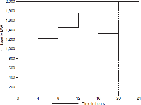
FIG. 4.1 Discrete levels of system load of daily load cycle
The problem of UC is nothing but to determine the units that should operate for a particular load. To ‘commit’ a generating unit is to ‘turn it on’, i.e., to bring it up to speed, synchronize it to the system, and connect it, so that it can deliver power to the network.
4.2 COMPARISON WITH ECONOMIC LOAD DISPATCH
Economic dispatch economically distributes the actual system load as it rises to the various units that are already on-line. However, the UC problem plans for the best set of units to be available to supply the predicted or forecast load of the system over a future time period.
4.3 NEED FOR UC
- The plant commitment and unit-ordering schedules extend the period of optimization from a few minutes to several hours.
- Weekly patterns can be developed from daily schedules. Likewise, monthly, seasonal, and annual schedules can be prepared by taking into consideration the repetitive nature of the load demand and seasonal variations.
- A great deal of money can be saved by turning off the units when they are not needed for the time. If the operation of the system is to be optimized, the UC schedules are required for economically committing units in plant to service with the time at which individual units should be taken out from or returned to service.
- This problem is of importance for scheduling thermal units in a thermal plant; as for other types of generation such as hydro, their aggregate costs (such as start-up costs, operating fuel costs, and shut-down costs) are negligible so that their on-off status is not important.
4.4 CONSTRAINTS IN UC
There are many constraints to be considered in solving the UC problem.
4.4.1 Spinning reserve
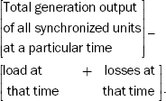
It is the term used to describe the total amount of generation available from all synchronized units on the system minus the present load and losses being supplied. Here, the synchronized units on the system may be named units spinning on the system.

Let PGsp be the spinning reserve, ![]() the power generation of the i th synchronized unit, PD the total load on the system, and pL the total loss of the system:
the power generation of the i th synchronized unit, PD the total load on the system, and pL the total loss of the system:
The spinning reserve must be maintained so that the failure of one or more units does not cause too far a drop in system frequency. Simply, if one unit fails, there must be an ample reserve on the other units to make up for the loss in a specified time period.
The spinning reserve must be a given a percentage of forecasted peak load demand, or it must be capable of taking up the loss of the most heavily loaded unit in a given period of time.
It can also be calculated as a function of the probability of not having sufficient generation to meet the load.
The reserves must be properly allocated among fast-responding units and slow-responding units such that this allows the automatic generation control system to restore frequency and quickly interchange the time of outage of a generating unit.
- Beyond the spinning reserve, the UC problem may consider various classes of ‘scheduled reserves’ or off-line reserves. These include quick-start diesel or gas-turbine units as well as most hydro-units and pumped storage hydro-units that can be brought on-line, synchronized, and brought upto maximum capacity quickly. As such, these units can be counted in the overall reserve assessment as long as their time to come up to maximum capacity is taken into consideration.
- Reserves should be spread well around the entire power system to avoid transmission system limitations (often called ‘bottling’ of reserves) and to allow different parts of the system to run as ‘islands’, should they become electrically disconnected.
4.4.2 Thermal unit constraints
A thermal unit can undergo only gradual temperature changes and this translates into a time period (of some hours) required to bring the unit on the line. Due to such limitations in the operation of a thermal plant, the following constraints are to be considered.
- Minimum up-time: During the minimum up-time, once the unit is operating (up state), it should not be turned off immediately.
- Minimum down-time: The minimum down-time is the minimum time during which the unit is in ‘down’ state, i.e., once the unit is decommitted, there is a minimum time before it can be recommitted.
- Crew constraints: If a plant consists of two or more units, they cannot both be turned on at the same time since there are not enough crew members to attend to both units while starting up.
Start-up cost
In addition to the above constraints, because the temperature and the pressure of the thermal unit must be moved slowly, a certain amount of energy must be expended to bring the unit on-line and is brought into the UC problem as a start-up cost.
The start-up cost may vary from a maximum ‘cold-start’ value to a very small value if the unit was only turned off recently, and it is still relatively close to the operating temperature.
Two approaches to treating a thermal unit during its ‘down’ state:
- The first approach (cooling) allows the unit’s boiler to cool down and then heat back up to a operating temperature in time for a scheduled turn-on.
- The second approach (banking) requires that sufficient energy be input to the boiler to just maintain the operating temperature.
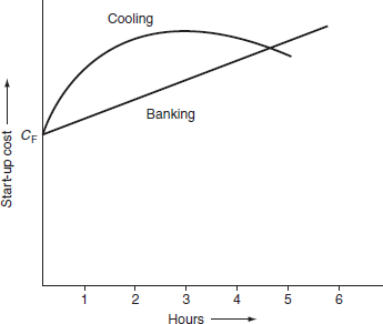
The best approach can be chosen by comparing the costs for the above two approaches.
Let CC be the cold-start cost (MBtu), C the fuel cost, CF the fixed cost (includes crew expenses and maintainable expenses), α the thermal time constant for the unit, Ct the cost of maintaining unit at operating temperature (MBtu/hr), and t the time the unit was cooled (hr).
Start-up cost when cooling = Cc (1 – e-t/α) C + CF;
Start-up cost when banking =Ct × t × C + CF.
Upto a certain number of hours, the cost of banking < cost of cooling is shown in Fig. 4.2.
The capacity limits of thermal units may change frequently due to maintenance or unscheduled outages of various equipments in the plant and this must also be taken into consideration in the UC problem.
The other constraints are as follows
4.4.3 Hydro-constraints
As pointed out already that the UC problem is of much importance for the scheduling of thermal units, it is not the meaning of UC that cannot be completely separated from the scheduling of a hydro-unit.
The hydro-thermal scheduling will be explained as separated from the UC problem. Operation of a system having both hydro and thermal plants is, however, far more complex as hydro-plants have negligible operation costs, but are required to operate under constraints of water available for hydro-generation in a given period of time.
The problem of minimizing the operating cost of a hydro-thermal system can be viewed as one of minimizing the fuel cost of thermal plants under the constraint of water availability for hydro-generation over a given period of operation.
4.4.4 Must run
It is necessary to give a must-run reorganization to some units of the plant during certain events of the year, by which we yield the voltage support on the transmission network or for such purpose as supply of steam for uses outside the steam plant itself.
4.4.5 Fuel constraints
A system in which some units have limited fuel or else have constraints that require them to burn a specified amount of fuel in a given time presents a most challenging UC problem.
4.5 COST FUNCTION FORMULATION
Let Fi be the cost of operation of the i th unit, PGi the output of the i th unit, and Ci the running cost of the i th unit. Then,
Fi = Ci PGi
Ci may vary depending on the loading condition.
Let Cij be the variable cost coefficient for the i th unit when operating at the j th load for which the corresponding active power is PGij.
Since the level of operation is a function of time, the cost efficiency may be described with yet another index to denote the time of operation, so that it becomes Cijt for the sub-interval ‘t’ corresponding to a power output of ![]() .
.
If each unit is capable of operation at k discrete levels, then the running cost Fit of the i th unit in the time interval t is given by
If there are n units available for operation in the time interval ‘t’, then the total running cost of n units during the time interval ‘t’ is
For the entire time period of optimization, having T sub-intervals of time, the overall running cost for all the units may become
4.5.1 Start-up cost consideration
Suppose that for a plant to be brought into service, an additional expenditure Csi has to be incurred in addition to the running cost (i.e., start-up cost of the i th unit), the cost of starting ‘x’ number of units during any sub-interval t is given by
where δit = 1, if the i th unit is started in sub-interval ‘t’ and otherwise δit = 0.
4.5.2 Shut-down cost consideration
Similarly, if a plant is taken out of service during the scheduling period, it is necessary to consider the shut-down cost.
If ‘y’ number of units are be to shut down during the sub-interval ‘t’, the shut-down cost may be represented as
where σit = 1, when the i th unit is thrown out of service in sub-interval ‘t’; otherwise σit = 0.
Over the complete scheduling period of T sub-intervals, the start-up cost is given by
and the shut-down cost is
Now, the total expression for the cost function including the running cost, the start-up cost, and the shut-down cost is written in the form:
For each sub-interval of time t, the number of generating units to be committed to service, the generators to be shut down, and the quantized power loading levels that minimize the total cost have to be determined.
4.6 CONSTRAINTS FOR PLANT COMMITMENT SCHEDULES
As in the optimal point generation scheduling, the output of each generator must be within the minimum and maximum value of capacity:
i.e.,
The optimum schedules of generation are prepared from the knowledge of the total available plant capacity, which must be in excess of the plant-generating capacity required in meeting the predicted load demand in satisfying the requirements for minimum running reserve capacity during the entire period of scheduling:
where STAC is the total available capacity in any sub-interval ‘t’, Srmin the minimum running reserve capacity, αit = 1, if the i th unit is in operation during sub-interval ‘t’; otherwise αit = 0
In addition, for a predicted load demand PD, the total generation output in sub-interval ‘t’ must be in excess of the load demand by an amount not less than the minimum running reserve capacity Srmin.
![]() (without considering the transmission losses)
(without considering the transmission losses)
In case of consideration of transmission losses, the above equation becomes
The generator start-up and shut-down logic indicators δit and σit, respectively, should be unity during the corresponding sub-intervals of operation
4.7 UNIT COMMITMENT—SOLUTION METHODS
The most important techniques for the solution of a UC problem are:
- Priority-list schemes.
- Dynamic programming (DP) method.
- Lagrange’s relaxation (LR) method.
Now, we will explain the priority-list scheme and the DP method.
A simple shut-down rule or priority-list scheme could be obtained after an exhaustive enumeration of all unit combinations at each load level.
4.7.1 Enumeration scheme
A straightforward but highly time-consuming way of finding the most economical combination of units to meet a particular load demand is to try all possible combinations of units that can supply this load. This load is divided optimally among the units of each combination by the use of co-ordination equations so as to find the most economical operating cost of the combination. Then, the combination that has the least operating cost among all these is determined.
Some combinations will be infeasible if the sum of all maximum MW for the units committed is less than the load or if the sum of all minimum MW for the units committed is greater than the load.
Example 4.1: Let us consider a plant having three units. The cost characteristics and minimum and maximum limits of power generation (MW) of each unit are as follows:
Unit-1,
C1 = 0.002842P2G1 + 8.46 PG1 + 600.0 Rs./hr, 200 ≤ PG1 ≤ 650
Unit-2,
C2 = 0.002936P2G2 + 8.32 PG2 + 420.0 Rs./hr, 150 ≤ PG2 ≤ 450
Unit-3,
C3 = 0.006449P2G3 + 9.884 PG3 + 110.0 Rs./hr, 100 ≤ PG3 ≤ 300
To supply a total load of 600 MW most economically, the combinations of units and their generation status are tabulated in Table 4.1.
Number of combinations = 2n =23 = 8

Note: The least expensive was not to supply the generation with all three units running or even any combination involving two units. Rather, the optimum commitment was to run only unit-1, the most economic unit. By only running it, the load can be supplied by that unit operating closer to its best efficiency. If another unit is committed, both Unit-1 and the other unit will be loaded further from their best efficiency points such that the net cost is greater than unit-1 alone.
4.7.1.1 UC operation of simple peak–valley load pattern: shut-down rule
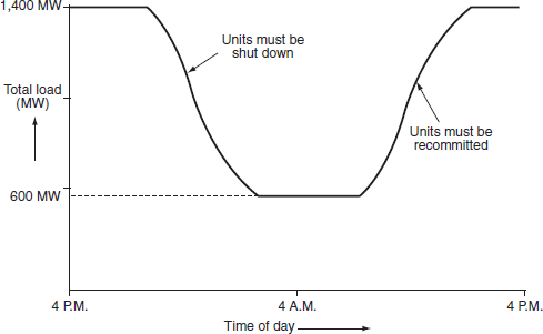
Let us assume that the load follows a simple ‘peak–valley’ pattern as shown in Fig. 4.3.
To optimize the system operation, some units must be shut down as the load decreases and is then recommitted (put into service) as it goes back up.
One approach called the ‘shut-down rule’ must be used to know which units to drop and when to drop them. A simple priority-list scheme is to be developed from the ‘shut-down rule’.
Consider the example, with the load varying from a peak of 1,400 MW to a valley of 600 MW (Table 4.2). To obtain a ‘shut-down rule’, we simply use a brute-force technique wherein all combinations of units will be tried for each load level taken in steps of some MW (here 50 MW).
TABLE 4.2 Shut-down rule derivation

From the above table, we can observe that for the load above 1,100 MW, running all the three units is economical; between 1,100 and 700 MW running the first and second units is economical. For below 700 MW, running of only Unit-1 is economical as shown in Fig. 4.4.
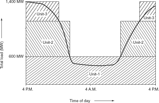
FIG. 4.4 UC schedule using the shut-down rule

TABLE 4.4 Priority list for supply of 1,400 MW
| Combination of units | For combination PGmin | For combination PGmax |
|---|---|---|
2, 1, and 3 |
50 |
1,400 |
2 and 1 |
350 |
1,100 |
2 |
150 |
450 |
4.7.2 Priority-list method
A simple but sub-optimal approach to the problem is to impose priority ordering, wherein the most efficient unit is loaded first to be followed by the less efficient units in order as the load increases.
In this method, first we compute the full-load average production cost of each unit. Then, in the order of ascending costs, the units are arranged to commit the load demand.
For Example 4.1, we construct a priority list as follows:
First, the full-load average production cost will be calculated.
The full-load average production cost of Unit-1 = 9.79 Rs./MWh.
The full-load average production cost of Unit-2 = 9.48 Rs./MWh.
The full-load average production cost of Unit-3 = 11.188 Rs./MWh.
A priority order of these units based on the average production is as follows (Table 4.3):
By neglecting minimum up- or down-time, start-up costs, etc. the load demand can be met by the possible combinations as follows (Table 4.4):
4.7.2.1 Priority-list scheme versus shut-down sequence
In shut-down sequence, Unit-2 was shut down at 700 MW leaving Unit-1. With the priority-list scheme, both units would be held ON until the load had reached 450 MW and then Unit-1 would be dropped.
Many priority-list schemes are made according to a simple shut-down algorithm, such that they would have steps for shutting down a unit as follows:
- During the dropping of load, at the end of each hour, determine whether the next unit on the priority list will have sufficient generation capacity to meet the load demand and to satisfy the requirement of the spinning reserve. If yes go to the next step and otherwise continue the operation with the unit as it is.
- Determine the time in number of hours ‘h’ before the dropped unit (in Step 1) will be needed again for service.
- If the number of hours (h) is less than minimum shut-down time for the unit, then keep the commitment of the unit as it is and go to Step 5; if not, go to the next step.
- Now, calculate the first cost, which is the sum of hourly production costs for the next ‘h’ hours with the unit in ‘up’ state. Then, recalculate the same sum as second cost for the unit ‘down’ state and in the start-up cost for either cooling the unit or banking it, whichever is less expensive. If there are sufficient savings from shutting down the unit, it should be shut down, otherwise keep it on.
- Repeat the above procedure for the next unit on the priority list and continue for the subsequent unit.
The various improvements to the priority-list schemes can be made by grouping of units to ensure that various constraints are met.
4.7.3 Dynamic programming
Dynamic programming is based on the principle of optimality explained by Bellman in 1957. It states that ‘an optimal policy has the property, that, whatever the initial state and the initial decisions are, the remaining decisions must constitute an optimal policy with regard to the state resulting from the first decision’.
This method can be used to solve problems in which many sequential decisions are required to be taken in defining the optimum operation of a system, which consists of a distinct number of stages. However, it is suitable only when the decisions at the later stages do not affect the operation at the earlier stages.
4.7.3.1 Solution of an optimal UC problem with DP method
Dynamic programming has many advantages over the enumeration scheme, the main advantage being a reduction in the size of the problem.
The imposition of a priority list arranged in order of the full-load average cost rate would result in a correct dispatch and commitment only if
- No–load costs are zero.
- Unit input–output characteristics are linear between zero output and full load.
- There are no other limitations.
- Start-up costs are a fixed amount.
In the DP approach, we assume that:
- A state consists of an array of units with specified operating units and the rest are at off-line.
- The start-up cost of a unit is independent of the time if it has been off-line.
- There are no costs for shutting down a unit.
- There is a strict priority order and in each interval a specified minimum amount of capacity must be operating.
A feasible state is one at which the committed units can supply the required load and that meets the minimum amount of capacity in each period.
Practically, a UC table is to be made for the complete load cycle. The DP method is more efficient for preparing the UC table if the available load demand is assumed to increase in small but finite size steps. In DP it is not necessary to solve co-ordinate equations, while at the same time the unit combinations are to be tried.
Considerable computational saving can be achieved by using the branch and bound technique or a DP method for comparing the economics of combinations as certain combinations need not be tried at all.
The total number of units available, their individual cost characteristics, and the load cycle on the station are assumed to be known a priori. Further, it shall be assumed that the load on each unit or combination of units changes in suitably small but uniform steps of size ∆ MW (say 1 MW).
Procedure for preparing the UC table using the DP approach:
Step 1: |
Start arbitrarily with consideration of any two units. |
Step 2: |
Arrange the combined output of the two units in the form of discrete load levels. |
Step 3: |
Determine the most economical combination of the two units for all the load levels. It is to be observed that at each load level, the economic operation may be to run either a unit or both units with a certain load sharing between the two units. |
Step 4: |
Obtain the most economical cost curve in discrete form for the two units and that can be treated as the cost curve of a single equivalent unit. |
Step 5: |
Add the third unit and repeat the procedure to find the cost curve of the three combined units. It may be noted that by this procedure, the operating combinations of the third and first and third and second units are not required to be worked out resulting in considerable saving in computation. |
Step 6: |
Repeat the process till all available units are exhausted. |
The main advantage of this DP method of approach is that having obtained the optimal way of loading ‘K’ units, it is quite easy to determine the optimal way of loading (K + 1) units.
Mathematical representation
Let a cost function FN (x) be the minimum cost in Rs./hr of generation of ‘x’ MW by N number of units, fN (y) the cost of generation of ‘y’ MW by the N th unit, and FN −1 (x − y) the minimum cost of generation of (x − y) MW by remaining (N − 1) units.
The following recursive relation will result with the application of DP:
The most efficient economical combination of units can efficiently be determined by the use of the above relation. Here the most economical combination of units is such that it yields the minimum operating cost, for discrete load levels ranges from the minimum permissible load of the smallest unit to the sum of the capacities of all available units.
In this process, the total minimum operating cost and the load shared by each unit of the optimal combination are automatically determined for each load level.
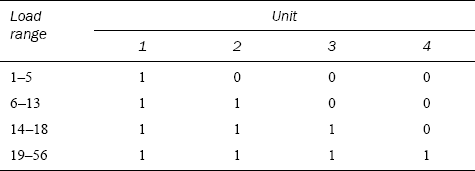
Example 4.2: A power system network with a thermal power plant is operating by four generating units. Determine the most economical unit to be committed to a load demand of 8 MW. Also, prepare the UC table for the load changes in steps of 1 MW starting from the minimum to the maximum load. The minimum and maximum generating capacities and cost-curve parameters of the units listed in a tabular form are given in Table 4.5.
Solution:
We know that:
The cost function,
Incremental fuel cost,
The total load = PD = 8 MW (given)
By comparing the cost-curve parameters, we come to know that the cost characteristics of the first unit are the lowest. If only one single unit is to be committed, Unit-1 is to be employed.
Now, find out the cost of generation of power by the first unit starting from minimum to maximum generating capacity of that unit.
Let,
f1(1) = the main cost in Rs./hr for the generation of 1 MW by the first unit
f1(2) = the main cost in Rs./hr for the generation of 2 MW by the first unit
f1(3) = the main cost in Rs./hr for the generation of 3 MW by the first unit
f1(4) = the main cost in Rs./hr for the generation of 4 MW by the first unit
….. ….. ….. ….. … … … … … … … … …
f1(8) = the main cost in Rs./hr for the generation of 8 MW by the first unit

TABLE 4.5 Capacities and cost-curve parameters of the units

For the commitment of Unit-1 only
When only one unit is to be committed to meet a particular load demand, i.e., Unit-1 in this case due to its less cost parameters, then F1(x) = f1(x).
where:
F1(x) is the minimum cost of generation of ‘x’ MW by only one unit
f1(x) is the minimum cost of generation of ‘x’ MW by Unit-1
∴F1(1) = f1(1) = (0.37 × 1 + 22.9) 1 = 23.27
F1(2) = f1(2) = (0.37 × 2 + 22.9) 2 = 47.28
F1(3) = f1(3) = (0.37 × 3 + 22.9) 3 = 72.03
Similarly,
F1(4) = f1(4) = 97.52
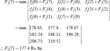
F1(5) = f1(5) = 123.75
F1(6) = f1(6) = 150.72
F1(7) = f1(7) = 178.43
F1(8) = f1(8) = 206.88
When Unit-1 is to be committed to meet a load demand of 8 MW, the cost of generation becomes 206.88 Rs./hr.
For the second unit
f2(1) = min. cost in Rs./hr for the generation of 1 MW by the second unit only
= (0.78PG2 + 25.9) PG2
= (0.78 × 1 + 25.9) 1 = 26.68
Similarly,
f2(2) = 54.92
f2(3) = 84.72
f2(4) = 116.08
f2(5) = 149.0
f2(6) = 183.48
f2(7) = 219.52
f2(8) = 257.12
By observing f1(8) and f2(8), it is concluded that f1(8) < f2(8), i.e., the cost of generation of 8 MW by Unit-1 is minimum than that by Unit-2.
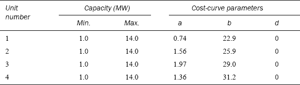
For commitment of Unit-1 and Unit-2 combination
F2(8) = Minimum cost of generation of 8 MW by the simultaneous operation of two units
i.e., Units-1 and 2.
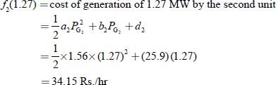
In other words, the minimum cost of generation of 8 MW by the combination of Unit-1 and Unit-2 is 205.11 Rs./hr and for this optimal cost, Unit-1 supplies 7 MW and Unit-2 supplies 1 MW.
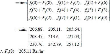
i.e., the minimum cost of generation of 7 MW with the combination of Unit-1 (by 6-MW supply) and Unit-2 (by 1-MW supply) is 177.4 Rs./hr.


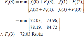
F2(2) |
= |
min [f2(0) + F1(2), f2(1) + F1(1), f2(2) + F1(0)] |
|
= |
min [47.28, 49.95, 54.92] |
∴ F2(2) |
= |
47.28 Rs./hr |
F2(1) |
= |
min [f2(0) + F1(1), f2(1) + F1(0)] |
|
= |
min [23.27, 26.68] |
∴ F2(1) |
= |
23.27 Rs./hr |
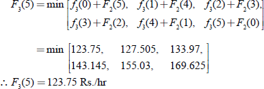
Now, the cost of generation by Unit-3 only is

f3(0) = 0; |
f3(5) = 169.625 |
f3(1) = 29.985; |
f3(6) = 209.46 |
f3(2) = 61.94; |
f3(7) = 251.265 |
f3(3) = 95.865; |
f3(8) = 295.04 |
f3(4) = 131.76; |
|
For commitment of Unit - 1, Unit - 2, and Unit-3 combination
F3(8) = The minimum cost of generation of 8 MW by the three units, i.e., Unit-1, Unit-2, and Unit-3

i.e., for the generation of 8 MW by three units, Unit-1 and Unit-2 will commit to meet the load of 8 MW with Unit-1 supplying 7 MW, Unit-2 supplying 1 MW, and Unit-3 is in an off-state condition.


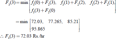
F3(2) |
= |
min [f3(0) + F2(2), f3(1) + F2(1), f3(2) + F2(0)] |
|
= |
min [47.28, 53.255, 61.94] |
∴ F3(2) |
= |
47.28 Rs./hr |
F3(1) |
= |
min [ f3(0) + F2(1), f3(1) + F2(0)] |
|
= |
min [23.27, 29.958] |
∴ F3(1) |
= |
23.27 Rs./hr |
Cost of generation by the fourth unit

f4(0) = 0
f4(1) = 31.88 Rs./hr
f4(2) = 65.12 Rs./hr
f4(3) = 99.72 Rs./hr
f4(4) = 135.68 Rs./hr
f4(5) = 173.0 Rs./hr
f4(6) = 211.68 Rs./hr
f4(7) = 251.72 Rs./hr
f4(8) = 293.12 Rs./hr
Minimum cost of generation by four units, i.e., Unit-1, Unit-2, Unit-3, and Unit-4
F4(8) = The minimum cost of generation of 8 MW by four units

i.e., for the generation of 8 MW by four units, Unit-1 and Unit-2 will commit to meet the load of 8 MW with Unit-1 supplying 7 MW, Unit-2 supplying 1 MW, and Unit-3 as well as Unit-4 are in an off-state condition:


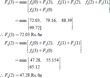
F4(1) |
= |
min [f4(0) + F3(1), f4(1) + F3(0)] |
|
= |
min [23.27 31.88] |
∴ F4(1) |
= |
23.27 Rs./hr |
From the above criteria, it is observed that for the generation of 8 MW, the commitment of units is as follows:
f1 (8) |
= |
F1(8) = the minimum cost of generation of 8 MW in Rs./hr by Unit-1 only |
|
= |
206.88 Rs./hr |
F2(8) |
= |
the minimum cost of generation of 8 MW by two units with Unit-1 supplying 7 MW and Unit-2 supplying 1 MW |
|
= |
205.11 Rs./hr |
= |
the minimum cost of generation of 8 MW by three units with Unit-1 supplying 7 MW, Unit-2 supplying 1 MW, and Unit-3 is in an off-state condition. |
|
|
= |
205.11 Rs./hr |
F4(8) |
= |
minimum cost of generation of 8 MW by four units with Unit-1 supplying 7 MW, Unit-2 supplying 1MW, and Unit-3 and Unit-4 are in an off-state condition. |
|
= |
205.11 Rs./hr |
By examining the costs F1(8), F2(8), F3(8), and F4(8), we have concluded that for meeting the load demand of 8 MW, the optimal combination of units to be committed is Unit-1 with 7 MW and Unit-2 with 1 MW, respectively, at an operating cost of 205.11 Rs./hr
For preparing the UC table, the ordering of units is not a criterion. For any order, we get the same solution that is independent of numbering units.
To get a higher accuracy, the step size of the load is to be reduced, which results in a considerable increase in time of computation and required storage capacity.
Status 1 of any unit indicates unit running or unit committing and status 0 of any unit indicates that the unit is not running.
The UC table is prepared once and for all for a given set of units (Table 4.6). As the load cycle on the station changes, it would only mean changes in starting and stopping of units without changing the basic UC table.
The UC table is used in giving the information of which units are to be committed to supply a particular load demand. The exact load sharing between the units committed is to be obtained by solving the co-ordination equations as below.
Total load,

|
PG1 = PG2 = 8 MW (given) |
(4.5) |
|
⇒ PG2 = 8 − PG1 |
|
TABLE 4.6 The UC table for the above-considered system
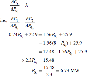
i.e., load shared by the first unit, PG1 = 6.73 MW
and PG2 − 8 − PG1 = 8 − 6.73 = 1.27 MW
i.e., load shared by the second unit, PG2 = 1.27 MW
Lagrangian multiplier, λ |
= |
0.74PG1 + 22.9 = 1.56PG2 + 25.9 |
|
= |
27.88 Rs./MWh |

The total minimum operating cost with an optimal combination of Unit-1 and Unit-2 is
f1 + f2 = 205.11 Rs./hr
To prepare the UC table, the load is to vary in steps of 1 MW starting from a minimum generating capacity to a maximum generating capacity of a station in suitable steps.
4.8 CONSIDERATION OF RELIABILITY IN OPTIMAL UC PROBLEM
In addition to the economy of power generation, the reliability or continuity of power supply is also another important consideration. Any supply undertaking has assured all its consumers to provide reliable and quality of service in terms of the specified range of voltage and frequency.
The aspect of reliability in addition to economy is to be properly co-ordinated in preparing the UC table for a given system.
The optimal UC table is to be modified to include the reliability considerations.
Sometimes, there is an occurrence of the failure of generators or their derating conditions due to small and minor defects. Under that contingency of forced outage, in order to meet the load demand, ‘static reserve capacity’ is always maintained at a generating station such that the total installed capacity exceeds the yearly peak demand by a certain margin. This is a planning problem.
In arriving at the economic UC decision at any particular period, the constraint taken into consideration was merely a fact that the total generating capacity on-line was at least equal to the total load demand. If there was any margin between the capacity of units committed and the load demand, it was incidental. Under actual operation, one or more number of units had failed randomly; it may not be possible to meet the load demand for a certain period of time. To start the spare (standby) thermal unit and to bring it on the line to take up the load will involve long periods of time usually from 2 to 8 hr and also some starting cost. In case of a hydro-generating unit, it could be brought on-line in a few minutes to take up the load.
Hence, to ensure continuity of supply to meet random failures, the total generating capacity on-line must have a definite margin over the load requirements at any point of time. This margin is called the spinning reserve, which ensures continually by meeting the demand upto a certain extent of probable loss of generating capacity. While rules of thumb have been used, based on past experience to determine the system spinning reserve at any time, a recent better approach called Patton’s analytical approach is the most powerful approach to solve this problem.
Consider the following points in the aspect of reliability consideration in the UC problem:
- The probability of outage of any unit that increases with its operating time and a unit, which is to provide a spinning reserve at any particular time, has to be started several hours later. Hence, the security of supply problem has to be treated in totality over a period of one day.
- The loads are never known with complete certainty.
- The spinning reserve has to be facilitated at suitable generating stations of the system and not necessarily at each generating station.
A unit’s useful life span undergoes alternate periods of operation and repair as shown in Fig. 4.5.
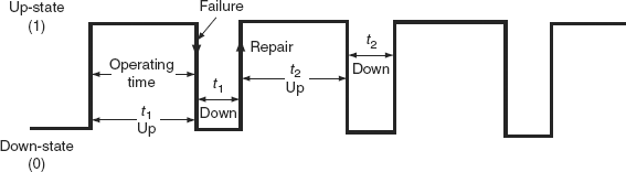
FIG. 4.5 Random outage phenomena of a generating unit excluding the scheduled outages
A unit operating time is also called unit ‘up-time’ (tup) and its repair time as its ‘down-time’ (tdown).
The lengths of individual operating and repair periods are a random phenomenon with much longer periods of operation compared to repair periods.
This random phenomenon with a longer operating period of a unit is described by using the following parameters.
Mean time to failure (mean ‘up’ time):
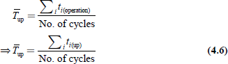
Mean time to repair (mean ‘down’ time):
∴ Mean cycle time = ![]()
The rate of failure and the rate of repair can be defined by inversing Equations (4.6) and (4.7) as
Rate of failure ![]() failures/year
failures/year
Rate of repair ![]() repairs/year
repairs/year
The failure and repair rates are to be estimated from the past data of units or other similar units elsewhere.
The rates of failure are affected by relative maintenance and the rates of repair are affected by the size, composition, and skill of repair teams.
By making use of the ratio definition of generating units, the probability of a unit being in an ‘up’ state and ‘down’ state can be expressed as
Probability of the unit in the ‘up’ state is

The probability of the unit in the ‘down’ state is

Obviously, Pup + Pdown = 1 (4.10)
Pup and Pdown are also known as availability and unavailability of the unit.
In any system with k number of units, the probability of the system state changes, i.e., when k units are present in a system, the system state changes due to random outages.
The random outage (failure) of a unit can be considered as an event independent of the state of the other unit.
Let a particular system state ‘i’, in which xi units are in the ‘down’ state and yi units are in the ‘up’ state:
i.e., xi + yi = k
The probability of the system being in state ‘i’ is expressed as
Π indicates probability multiplication of the system state.
4.8.1 Patton’s security function
Some intolerable or undesirable condition of system operation is termed as a ‘breach of system security’.
In an optimal UC problem, the only breach of security considered is the insufficient generating capacity of the system at a particular instant of time.
The probability that the available generating capacity at a particular time is less than the total load demand on the system at that time is complicatively estimated by one function known as Patton’s security function.
Patton’s security function is defined as
where Pi is the probability of the system being in the i th state and ri is the probability that the system state i causes a breach of system security.
In considering all possible system states to determine the security function, from the practical point of view, this sum is to be taken over the states in which not more than two units are on forced outage, i.e., states with more than two units out may be neglected as the probability of their occurrence will be too small.
ri = 1, if the available generating capacity (sum of capacities of units committed) is less than the total load demand, i.e., ![]() . Otherwise ri=0.
. Otherwise ri=0.
The security function S gives a quantitative estimation of system insecurity.
4.9 OPTIMAL UC WITH SECURITY CONSTRAINT
From a purely economical point of view, a UC table is prepared from which we know which units are committed for a given load on the system.
For each period, we will estimate the security function
For any system, we will define maximum tolerable insecurity level (MTIL). This is a management decision and the value is based on past experience.
Whenever the security function exceeds MTIL (S > MTIL), it is necessary to modify the UC table to include the aspects of security. It is normally achieved by committing the next most economical unit to supply the load. With the new unit being committed, we will estimate the security function and check whether it is S < MTIL.
The procedure of committing the next most economical unit is continued upto S < MTIL. If S = MTIL, the system does not have proper reliability. Adding units goes upto one step only because for another, it is not necessary to add the next units more than one unit since there is a presence of spinning reserve.
4.9.1 Illustration of security constraint with Example 4.2
Reconsider Example 4.2 and the daily load curve for the above system as given in Fig. 4.6.
The economically optimal UC for this load curve is obtained by the use of the UC Table 4.6 (which was previously prepared) (Table 4.7).
Considering period E, in which the minimum load is 5 MW and Unit-1 is being committed to meet the load. We will check for this period whether the system is secure or not.
Assume the rate of repair, µ = 99 repairs/year
And rate of failure, λ = 1 failure/year for all four units
And also assume that MTIL = 0.005
We have to estimate the security function S for this period E:
Value of ri depending on whether there is a breach of security or not.
There are two possible states for Unit-1:
operating state (or) ‘up’ state
(or)
forced outage state (or) ‘down’ state
The probability of Unit-1 being in the ‘up’ state,

FIG. 4.6 Daily load curve
TABLE 4.7 Economically optimal UC table for load curve shown in Fig. 4.4

r1 = 0, since the generation of Unit-1 (max. capacity) is greater than the load (i.e.,14 MW > 5 MW).
There is no breach of security when the Unit-1 is in the ‘up’ state.
The probability of Unit-1 being in the ‘down’ state:
r2=1, since Unit-1 is in the down state (PG1 = 0), the load demand of 5 MW cannot be met.
There is a breach of security when Unit-1 is in the ‘down’ state. Now, find the value of the security function.
where i represents the state of Unit-1.
If n is the number of units, number of states = 2n
For n = 1, states = 21 = 2 (i.e., up and down states)
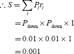
∴ S = P1 r1 + P2 r2
= P1up r1 + P1down r2
= 0.99 × 0 + 0.01 × 1
= 0.01
It is observed that 0.01 > 0.005, i.e., S > MTIL
Since in this case, S > MTIL represents system insecurity. Therefore, it is necessary to commit the next most economical unit, i.e., unit-2, to improve the security. When both Units-1 and 2 are operating, estimate the security function as follows:
Here, number of units, n = 2
∴ Number of states = 2n = 22 = 4
ri = 0, represents no breach of security and
ri = 1, represents breach of security

When taking either up down up combinations of states,
down up up
there is no breach of security, since ri=0
For the combination down
down,
there is a breach of security (Table 4.8).
It is observed that 0.001 < 0.005
Therefore, the combination of Unit-1 and Unit-2 does meet the MTIL of 0.005.
For all other periods of a load cycle, check whether the security function is less than MTIL. It is also found that for all other periods except E, the security function is less than MTIL. Now, we will obtain the optimal and security-constrained UC table for Example 4.2 (Table 4.9).
4.10 START-UP CONSIDERATION
From the optimal and secured UC table given in Table 4.9, depending on the load in a particular period, it is observed that some units are to be decommitted and restarted in the next period. Whenever a unit is to be restarted, it involves some cost as well as some time before the unit is put on-line. For thermal units, it is necessary to build up certain temperature and pressure gradually before the unit can supply any load demand. The cost involved in restarting any unit after the decommitting period is known as START-UP cost.
TABLE 4.9 Optimal and secure UC table for Example 4.2

* Unit is committed from the point of view of security considerations.
Depending on the condition of the unit, the start-up costs will be different. If the unit is to be started from a cold condition and brought upto normal temperature and pressure, the start-up costs will be maximum since some energy is required to build up the required pressure and temperature of the steam. Sometimes, the unit may be switched off and the temperature of steam may not be in a cold condition. This particular condition is called the banking condition.
From the UC table given in Table 4.7, it is observed that during Period B, Unit-3 is operating and during Period C, it is decommitted. It is restarted during Period D.
In Period C, check whether it is economical to run only two units or allow all the three units (Units-1, 2, and 3) to continue to run such that the start-up costs are eliminated.
Let us assume that the start-up cost of each unit=Rs. 500.
Case A: Unit-3 is not in operation in Period C, i.e., only two Units-1 and 2 are operating.
For Period B or D, total load = 15 MW
This is to be shared by three units, i.e., PG1 + PG2 + PG3 = 15
Subtracting Equation (4.14) from Equation (4.13), we get
Subtracting Equation (4.15) from Equation (4.13), we get
0.74PG1 − 1.97PG3 = 6.1 (4.17)
or 0.74PG1 − 1.97(15 − PG1 − PG2) = 6.1
or 2.71PG1 + 1.97PG2 = 35.65 (4.18)
By solving Equations (4.13) and (4.16), we have
PG1 = 10.8 MW, PG2 = 3.2 MW
PG3 = 15 − PG1 − PG2 = 15 − 108 − 3.2 = 1 MW
C1 = (0.37PG1 + 22.9)PG1 = 290.48 Rs./hr
C2 = (0.78PG2 + 25.9)PG2 = 90.87 Rs./hr
C3 = (0.985PG3 + 29)PG3 = 29.98 Rs./hr
For Period B, the operating time is 4 hr.
∴ Total cost, C = [C1 + C2 + C3] t
= [290.48 + 90.87 + 29.98] × 4
= Rs. 1,645.34
Total operating cost during Period B is Rs. 1,645.34.
In Period C, 10 MW of load is to be shared by Units-1 and 2
i.e., PG1 + PG2 = 10 MW (4.19)
By solving Equations (4.16) and (4.19), we get
PG1 = 8.086 MW and PG2 = 1.913 MW
Total operating cost for Period C
= [(0.37PG1 + 22.9)PG1 + (0.78PG2 + 25.9)PG2] × 4
= Rs. 1,047.05.
For period D, the total operating cost is the same as that of Period B = Rs. 1,645.34.
Therefore, the total operating cost for Periods B, C, and D is
= Rs. [1,645.34+1,047.05+1,645.34]
= Rs. 4,337.73.
In Period D, Unit-3 is restarted to commit the load, hence the start-up cost of Unit-3 is added to the total operating cost for periods B, C, and D:
Start-up cost for Unit-3 = Rs. 500 (given)
∴ Total cost of operating of units during period B, C, and D is
= 4,337.73+500
= Rs. 4,837.73
Case B : Unit-3 is allowed to run in Period C.
Hence, 10-MW load is to be shared by units 1, 2, and 3.
i.e., PG1 + PG2 + PG3 = 10 (4.20)
Substituting PG3 from Equation (4.20) in Equation (4.17), we get
0.74PG1 − 1.97(10 − PG1 − PG2) = 6.1 (4.21)
or 2.71PG1 + 1.97PG2 = 25.8 (4.22)
By solving Equations (4.16) and (4.21), we get
PG1 = 8.1 MW, PG2 = 1.9 MW, and PG3 = 0 MW
From the above powers, it is observed that PG3 violates the minimum generation capacity (i.e., 0 < 1).
Hence, set the generation capacity of Unit-3 at minimum capacity, i.e., PG3 = 1 MW.
Then the remaining 9 MW is optimally shared by Unit-1 and Unit-2 as
PG1 = 7.4 MW, PG2 = 1.6 MW, and PG3 = 1 MW
The operating cost at Period C
= [(0.37PG1 + 22.9)PG1 + (0.78PG2 + 25.9)PG2 + (0.985PG3 + 29)PG3] × 4 hr
= Rs. 1,048.57
Total cost for Periods B, C, and D = Rs. 1,645.34 + Rs. 1,048.57 + Rs. 1,645.34
= Rs. 4,339.25.
Rs. 4,339.25 < Rs. 4,837.73
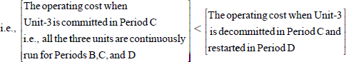
∴ It is concluded that to run Unit-3 in Period C is the economical way.
Now, the optimal UC table is modified as

* Unit is committed from the point of security consideration.
** Unit is committed from the point of start-up considerations.
Hence, it is economical to allow all the three units to continue to run in Periods B, C, and D, i.e., in Period C continuation of Unit-3 is economical.
Example 4.3: A power system network with a thermal power plant is operating by four generating units. Determine the most economical units to be committed to a load demand of 10 MW. Also prepare the UC table for the load changes in steps of 1 MW starting from the minimum to the maximum load. The minimum and maximum generating capacities and cost-curve parameters of the units listed in a tabular form are as given in Table 4.10.
Solution:
We know:
The cost function,
Incremental fuel cost,
The total load = PD = 10 MW (given)
By comparing the cost-curve parameters, we come to know that the cost characteristics of the first unit are the lowest. If only one single unit is to be committed, unit-1 is to be employed.

Now, find the cost-of-generation of power by the first unit starting from the minimum to the maximum generating capacity of that unit.
Let
f1(1) = the main cost in Rs./hr for the generation of 1 MW by the first unit
f1(2) = the main cost in Rs./hr for the generation of 2 MW by the first unit
f1(3) = the main cost in Rs./hr for the generation of 3 MW by the first unit
f1(4) = the main cost in Rs./hr for the generation of 4 MW by the first unit
….. ….. ….. ….. … … … … … … ….. ….. ….. … …
f1(10) = the main cost in Rs./hr for the generation of 10 MW by the first unit
For the commitment of Unit-1 only
When only one unit is to be committed to meet a particular load demand, i.e., Unit-1, in this case, due to its low cost parameters, then F1(x) = f1(x).
where
F1(x) is the minimum cost of generation of ‘x’ MW by only one unit
f1(x) is the minimum cost of generation of ‘x’ MW by Unit-1
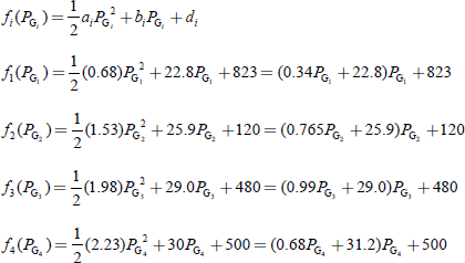
∴ F1(1) = f1(1) = (0.34×1+22.8) 1+823 = 846.14
F1(2) = f1(2) = (0.34×2+22.8) 2+823 = 869.96
F1(3) = f1(3) = (0.34×3+22.8) 3+823 = 894.46
F1(4) = f1(4) = 916.64
F1(5) = f1(5) = 945.50
F1(6) = f1(6) = 972.04
F1(7) = f1(7) = 996.26
F1(8) = f1(8) = 1,027.16
F1(9) = f1(9) = 1,055.74
F1(10) = f1(10) = 1,085.00
When Unit-1 is to be committed to meet a load demand of 10 MW, the cost of generation becomes 1,085 Rs./hr.
For the second unit:
f2(1) |
= |
minimum cost in Rs./hr for the generation of 1 MW by the second unit only |
|
= |
(0.765PG2 + 25.9)PG2 + 120 |
|
= |
(0.765 × 1 + 25.9)1 + 120 = 146.665 |
Similarly,
f2(2) = 174.860
f2(3) = 204.585
f2(4) = 235.840
f2(5) = 268.625
f2(6) = 302.940
f2(7) = 338.785
f2(8) = 376.160
f2(9) = 415.065
f2(10) = 455.500
By observing f1(10) and f2(10), it is concluded that f1(10) < f2(10), i.e., the cost of generation of 10 MW by unit-1 is minimum than that by Unit-2.
For commitment of unit-1 and Unit-2 combination
F2(10) = Minimum cost of generation of 10 MW by the simultaneous operation of two units, i.e., Units-1 and 2
In other words, the minimum cost of generation of 10 MW by the combination of Unit-1 and Unit-2 is 455.5 Rs./hr and for this optimal cost, Unit-1 supplies 0 MW and Unit-2 supplies 10 MW.
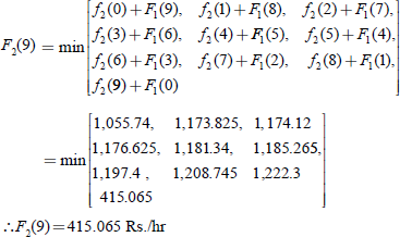
i.e., the minimum cost of generation of 9 MW with the combination of Unit-1 (by 0-MW supply) and Unit-2 (by 9-MW supply) is 415.065 Rs./hr.
Similarly,
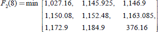
∴ F2(8) = 376.16 Rs./hr

∴F2(7) = 338.785 Rs./hr
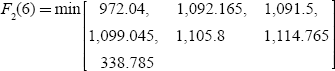
∴ F2(6) = 338.785 Rs./hr
∴F2(5) = 268.625 Rs./hr
∴F2(4) =235.84 Rs./hr
∴F2(3) =204.585 Rs./hr
∴F2(2) = 174.86 Rs./ hr
∴F2(1) = 146.665 Rs./hr
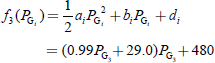
Now, the cost of generation by Unit-3 only:
f3(0) = 0; |
f3(5) = 649.75; f3(9) = 821.19 |
f3(1) = 509.99; |
f3(6) = 689.64; f3(10) = 869.00 |
f3(2) = 541.96; |
f3(7) = 731.51 |
f3(3) = 575.91; |
f3(8) = 775.36 |
f3(4) = 611.84; |
|
For commitment of Unit-1, Unit-2, and unit-3 combination:
F3(10) = The minimum cost of generation of 10 MW by the three units i.e., Unit-1, Unit-2, and Unit-3

i.e., for the generation of 10 MW by three Units, unit-2 alone will commit to meet the load of 10 MW and Units-1 and 3 are in an off-state condition:

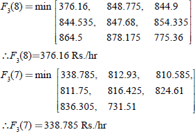
F3(3) = min [204.585, 684.85, 688.625, 575.91]
∴ F3(3) = 204.585 Rs./hr
F3(2) = min [174.86, 565.655, 541.96]
∴ F3(2) =174.86 Rs./hr
F3(1) = min [509.99, 146.665]
∴ F3(1) = 146.665 Rs./hr
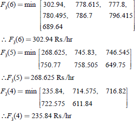
Cost of generation by the fourth unit

f4(0) = 0
f4(1) = 531.115 Rs./hr
f4(2) = 564.46 Rs./hr
f4(3) = 600.035 Rs./hr
f4(4) = 637.84 Rs./hr
f4(6) = 720.14 Rs./hr
f4(7) = 764.635 Rs./hr
f4(8) = 811.36 Rs./hr
f4(9) = 860.315 Rs./hr
f4(10) = 911.5 Rs./hr
Minimum cost of generation by four units, i.e., Unit-1, Unit-2, Unit-3, and Unit-4:
F4(10) = The minimum cost of generation of 10 MW by four units
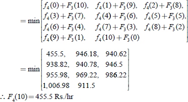
i.e., for the generation of 10 MW by four units, Unit-2 will commit to meet the load of 10 MW, and Unit-1, Unit-3, and Unit 4 are in an off-state condition:


F4(3) = min [204.585, 705.975, 711.125, 600.035]
∴F4 (3) = 204.585 Rs./hr
F4(2) = min [46.96, 554.255, 564.46]
∴F4(2) = 46.96 Rs./hr
F4(1) = min [23.14, 531.115]
∴F4(1) = 23.14 Rs./hr
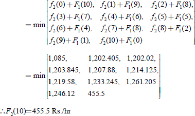
From the above criteria, it is observed that for the generation of 10 MW, the commitment of units is as follows:
f1(10) = F1(10) = the minimum cost of generation of 10 MW in Rs./hr by Unit-1 only
= 1085 Rs./hr
F2(10) = the minimum cost of generation of 10 MW by two units with Unit-1 supplying 0 MW and Unit-2 supplying 10 MW
= 455.5 Rs./hr
F3(10) = the minimum cost of generation of 10 MW by three units with Unit-2 supplying 10 MW, Unit-1 and Unit-3 is in an off-state condition
= 455.5 Rs./hr
F4(10) = the minimum cost of generation of 10 MW by four units with Unit-2 supplying 10 MW, and Unit-1, Unit-3 and Unit-4 are in an off-state condition
= 455.5 Rs./hr
By examining the costs F1(10), F2(10), F3(10), and F4(10), we have concluded that for meeting the load demand of 10 MW, the optimal combination of units to be committed is Unit-1, Unit-3, and Unit-4 in an off-state condition and Unit-2 supplying a 10-MW load at an operating cost of 455.5 Rs./hr.
For preparing the UC table, the ordering of units is not a criterion. For any order, we get the same solution that is independent of numbering units.
TABLE 4.11 The UC table for the above-considered system

To get a higher accuracy, the step size of the load is to be reduced, which results in considerable increase in time of computation and required storage capacity.
Status 1 of any unit indicates unit running or unit committing and Status 0 of any unit indicates unit not running.
The UC table is prepared once and for all for a given set of units (Table 4.11). As the load cycle on the station changes, it would only mean changes in starting and stopping of units without changing the basic UC table.
KEY NOTES
- Unit commitment is a problem of determining the units that should operate for a particular load.
- To ‘commit’ a generating unit is to ‘turn it on’.
- The constraints considered for unit commitment are:
- Spinning reserve.
- Thermal unit constraints.
- Hydro-constraints.
- Must-run constraints.
- Fuel constraints.
- The solution methods to a UC problem are:
- Priority-list scheme.
- Dynamic programming method (DP).
- Lagrange’s relaxation method (LR).
- In the priority ordering method, the most efficient unit is loaded first to be followed by the less efficient units in order as the load increases.
- The main advantage of the DP method is resolution in the dimensionality of problems, i.e., having obtained the optimal way of loading K number of units, it is quite easy to determine the optimal way of loading (K + 1) number of units.
MULTIPLE-CHOICE QUESTIONS
- Due to the load variation, it is not advisable to:
- Run all available units at all the times.
- Run only one unit at each discrete load level.
- Both (a) and (b).
- None of these.
- A unit when scheduled for connection to the system is said to be:
- Loaded.
- Disconnected.
- Committed.
- None of these.
- To determine the units that should operate for a particular load is the problem of:
- Unit commitment.
- Optimal load scheduling.
- Either (a) or (b).
- None of these.
- To commit a generating unit is:
- To bring it upto speed.
- To synchronize it to the system.
- To connect it so that it can deliver power to the network.
- All of these.
- Economic dispatch problem is applicable to various units, Which of the following is suitable?
- The units are already on-line.
- To supply the predicted or forecast load of the system over a future time period.
- Both (a) and (b).
- None of these.
- Unit commitment problem plans for the best set of units to be available. Which of the following is suitable?
- The units are already on-line.
- To supply the predicted or forecast load of the system over a future time period.
- Both (a) and (b).
- None of these.
- Spinning reserve is defined as:

- None of these.
- Spinning reserve must be:
- Maintained so that the failure of one or more units does not cause too far a drop in system frequency.
- Capable of taking up the loss of most heavily loaded unit in a given period of time.
- Calculated as a function of the probability of not having sufficient generation to meet the load.
- All of these.
- Because of temperature and pressure of thermal unit that must be moved slowly, a certain amount of energy must be expended to bring the unit on-line and is brought into the UC problem as a:
- Running cost.
- Fixed cost.
- Fuel cost.
- Start-up cost.
- Unit commitment problem is of much importance for:
- Scheduling of thermal units.
- Scheduling of hydro-units.
- Scheduling of both thermal and hydro-units.
- None of these.
- Thermal unit constraints considered in a UC problem are:
- Minimum up and minimum down times.
- Crew constraints.
- Start-up costs.
- All of these.
- The start-up cost may vary from a maximum cold-start value to a very small value if the thermal unit:
- Was only turned off recently.
- Is still relatively close to the operating temperature.
- Is still operating at normal temperature.
- Both (a) and (b).
- Unit commitment problem is:
- Of much importance for scheduling of thermal units.
- Cannot be completely separated from the scheduling of hydro-units.
- Used for hydro-thermal scheduling.
- Both (a) and (b).
- The constraints considered in a UC problem are:
- Thermal unit and hydro-unit constraints.
- Spinning reserve.
- Must-run and fuel constraints.
- All the above.
- The method used for obtaining the solution to a UC problem is:
- Priority-list scheme.
- Dynamic programming method.
- Lagrange’s relaxation method.
- All the above.
- A straightforward but highly time-consuming way of finding the most economical combination of units to meet a particular load demand is:
- Which is correct regarding the shut-down rule?
- To know which units to drop and when.
- From which a simple priority-list scheme is developed.
- Both (a) and (b).
- To know which units to start from shut-down condition.
- In the priority-list method of solving an optimal UC problem:
- Most efficient unit is loaded first to be followed by the less efficient unit in order as load increases.
- Less efficient unit is loaded first to be followed by the most efficient unit in order as load increases.
- Most efficient unit is loaded first to be followed by the less efficient unit in order as load decreases.
- Either (a) or (b).
- In the priority-list method, the units are arranged to commit the load demand in the order of:
- Ascending costs of units.
- Descending costs of units.
- Either (a) or (b).
- Independent of costs of units.
- The chief advantage of the DP method over the enumerate scheme is:
- Reduction in time of computation.
- Reduction in the dimensionality of the problem.
- Reduction in the number of units.
- All of these.
- In the DP method, the cost function FN(x) represents:
- Minimum cost in Rs/hr of generation of N MW by x number of units.
- Minimum cost in Rs/hr of generation of x MW by N number of units.
- Minimum cost in Rs/hr of generation of N MW by the xth unit.
- Minimum cost in Rs/hr of generation of x MW by the Nth unit.
- In the DP method, the cost function FN (y) represents:
- Cost of generation of N MW by y number of units.
- Cost of generation of y MW by N number of units.
- Cost of generation of N MW by the yth unit.
- Cost of generation of y MW by the Nth unit.
- The recursive relation results with the application of the DP method of solving the UC problem is:
- For preparing the UC table, which of the following is not a criterion?
- Ordering of units.
- Ordering of costs of units.
- Ordering of range of load.
- All of these.
- In a UC table, unit running or unit committing is indicated by:
- Status 0.
- Status 1.
- Status +.
- Status >.
- In a UC table, the status of the unit not running is indicated by:
- Status 0.
- Status 0.
- Status +.
- Status −.
- The unscheduled or maintenance outages of various equipments of a thermal plant must be taken into account in:
- Optimal scheduling problem.
- UC problem.
- Load frequency controlling problem.
- All of these.
- Unit up-time is nothing but:
- A unit operating time.
- A unit repair time.
- A unit total lifetime.
- A unit designing time.
- Unit down-time is nothing but:
- A unit operating time.
- A unit repair time.
- A unit total lifetime.
- A unit designing time.
- In reliability aspects of a UC problem, the lengths of an individual operating and repair periods of a unit considered at a random phenomenon with:
- Much longer periods of operation compared to repair periods.
- Much longer periods of repair compared to operation periods.
- Equal periods of operation and repair.
- Either (a) or (b).
- Mean up-time of a unit
 is:
is:
- Mean time to failure.
- Mean time to repair.
- Mean of failure and repair times.
- Mean of total time.
- Mean down-time of a unit
 is:
is:
- Mean time to failure.
- Mean time to repair.
- Mean of failure and repair times.
- Mean of total time.
- Mean cycle time of a unit is:
- Rate of failure of a unit is expressed as:
- Rate of repair of a unit is expressed as:
- The rate of failure of a unit affected by:
- Relative maintenance.
- Size, composition of repair team.
- Skill of repair team.
- All of these.
- The rate of repair of a unit is affected by:
- Relative maintenance.
- Size, composition of repair team.
- Skill of repair team.
- Both (b) and (c).
- Pup and Pdown of any unit represent:
- Unavailability and availability of a unit.
- Availability and unavailability of a unit.
- Either (a) or (b).
- Both (a) and (b).
- Pup+Pdown=
- Zero.
- 1.
- −1.
- Infinite.
- A breach of system security considered in optimal UC problem is:
- Use of Patton’s security function in the UC problem is the estimation of the probability that the available generating capacity at a particular time is:
- Less than the total load demand.
- More than the total load demand.
- Equal to the total load demand.
- Independent of the total load demand.
- Patton’s security function S gives a quantitative estimation of:
- System security.
- System insecurity.
- System stability.
- System variables.
- It is necessary to modify the UC table to include security aspects by committing the next most economical unit to supply the load when:
- S < MTIL.
- S > MTIL.
- S = MTIL.
- S = MTIL/2.
- The procedure of committing a most economical unit, to include security aspect in the UC table, is continued upto:
- S < MTIL.
- S > MTIL.
- S = MTIL.
- S = MTIL/2.
- System insecurity is represented by:
- S < MTIL.
- S > MTIL.
- S = MTIL.
- S = MITL/2.
- If the unit is to be started from a cold condition and brought upto normal temperature and pressure, the start-up cost will be:
- Minimum.
- Maximum.
- Having no effect.
- None of these.
- When any unit is in the UP state, there is:
- Breach of security.
- No breach of security.
- Stability.
- All of these.
- If
 the probability that the system state ‘i’ causes a breach of system security becomes:
- ri = 1.
- ri = 0.
- ri = −1.
- ri = ∞.
- If
 the probability that the system state ‘i’ causes a breach of system security becomes:
- ri=1.
- ri=0.
- ri = −1.
- ri= ∞.
SHORT QUESTIONS AND ANSWERS
- What is a UC problem?
It is not advisable to run all available units at all times due to the variation of load. It is necessary to decide in advance:
- Which generators to start up.
- When to connect them to the network.
- The sequence in which the operating units should be shut down and for how long.
The computational procedure for making the above such decisions is called the problem of UC.
- What do you mean by commitment of a unit?
To commit a generating unit is to turn it ON, i.e., to bring it upto speed, synchronize it to the system, and connect it, so that it can deliver power to the network.
- Why is the UC problem important for scheduling thermal units?
As for other types of generation such as hydro, the aggregate costs such as start-up costs, operating fuel costs, and shut-down costs are negligible so that their ON–OFF status is not important.
- Compare the UC problem with economic load dispatch.
Economic load dispatch economically distributes the actual system load as it rises to the various units already on-line. But the UC problem plans for the best set of units to be available to supply the predicted or forecast load of the system over future time periods.
- What are the different constraints that can be placed on the uc problem?
- Spinning reserve.
- Thermal unit constraints.
- Hydro-constraints.
- Must-run constraints.
- Fuel constraints.
- What are the thermal unit constraints considered in the UC problem?
The thermal unit constraints considered in the UC problem are:
- Minimum up-time.
- Minimum down-time.
- Crew constraints.
- Start-up cost.
- Why must the spinning reserve be maintained?
Spinning reserve must be maintained so that failure of one or more units does not cause too far a drop in system frequency, i.e., if one unit fails, there must be ample reserve on the other units to make up for the loss in a specified time period.
- Why are thermal unit constraints considered in a UC table?
A thermal unit can undergo only gradual temperature changes and this translates into a time period of some hours required to bring the unit on the line. Due to such limitations in the operation of a thermal plant, the thermal unit constraints are to be considered in the UC problem.
- What is a start-up cost and what is its significance?
Because of temperature and pressure of a thermal unit that must be moved slowly, a certain amount of energy must be moved slowly, a certain amount of energy must be expended to bring the unit on-line, and it is brought into the UC problem as a start-up cost.
The start-up cost may vary from a maximum cold-start value to a very small value if the unit was only turned off recently and is still relatively close to the operating temperature.
- Write the expressions of a start-up cost when cooling and when banking.
Start-up cost when cooling = Cc (1–e–t/α) C + CF
Start-up cost when banking = Ct × t × C + CF
where CC is the cold-start cost (MBtu), C is the fuel cost, CF is the fixed cost (includes crew expenses and maintainable expenses), α is the thermal time constant for the unit, Ct is the cost of maintaining a unit at operating temperature (MBtu/hr), and t is the time the unit was cooled (hr).
- What are the techniques used for getting the solution to the UC problem?
- Priority-list scheme.
- Dynamic programming (DP) method.
- Lagrange’s relaxation (LR) method.
- What are the steps of an enumeration scheme of finding the most economical combination of units to meet a load demand?
- To try all possible combinations of units that can supply the load.
- To divide this load optimally among the units of each combination by the use of co-ordination equations, so as to find the most economical operating cost of the combination.
- Then to determine the combination that has the least operating cost among all these.
- What is a shut-down rule of the UC operation?
If the operation of the system is to be optimized, units must be shut down as the load goes down and then recommitted as it goes back up. To know which units to drop and when, one approach called the shut-down rule must be used from which a simple priority-list scheme is developed.
- What is a priority-list method of solving a UC problem?
In this method, first the full-load average production cost of each unit, which is simply the net heat rate at full load multiplied by the fuel cost, is computed. Then, in the order of ascending costs, the units are arranged to commit the load demand.
- In a priority-list method, which unit is loaded first and to be followed by which units?
The most efficient unit is loaded first, to be followed by the less efficient units in the order as load increases.
- What is the chief advantage of the DP method over other methods in solving the UC problem?
Resolution in the dimensionality of problems, i.e., having obtained the optimal way of loading K number of units, it is quite easy to determine the optimal way of loading (K+1) number of units.
- What is the thermal constraint minimum up-time?
Minimum up-time is the time during which if the unit is running, it should not be turned off immediately.
- What is minimum down-time?
If the unit is stopped, there is a certain minimum time required to start it and put it on the line.
- What is spinning reserve?
To ensure the continuity of supply to meet random failures, the total generating capacity on-line must have a definite margin over the load requirements at any point of time. This margin is called spinning reserve, which ensures continuation by meeting the demand upto a certain extent of probable loss of generating capacity.
- What do you mean by a breach of system security?
Some intolerable or undesirable conditions of system operation is termed as a breach of system security.
- In an optimal UC problem, what is considered as a breach of security?
Insufficient generating capacity of the system at a particular instant of time.
- What is Patton’s security function? Give its expression.
Patton’s security function estimates the probability that the available generating capacity at a particular time is less than the total load demand on the system at that time.
It is expressed as

where Pi is the probability of the system being in the i th state and ri the probability that the system state ‘i ’ causes a breach of system security.
- How the optimal UC table is modified with consideration of security constraints?
Whenever the security function exceeds MTIL (S >MTIL), the UC table is modified by committing the next most economic unit to supply the loads. With the new unit being committed, the security function is then estimated and checked whether it is S < MTIL or not.
- What is the significance of must-run constraints considered in preparing the UC table?
Some units are given a must-run recognization during certain times of the year for the reason of voltage support on the transmission network or for such purposes as supply of steam for uses outside the steam plant itself.
REVIEW QUESTIONS
- Using the DP method, how do you find the most economical combination of the units to meet a particular load demand?
- Explain the different constraints considered in solving a UC problem.
- Compare an optimal UC problem with an economical load dispatch problem.
- Explain the need of an optimal UC problem.
- Describe the reliability consideration in an optimal UC problem.
- Describe the start-up cost consideration in an optimal UC problem.
PROBLEMS
- A power system network with a thermal power plant is operating by four generating units. Determine the most economical unit to be committed to a load demand of 10 MW. Prepare the unit commitment table for the load changes in steps of 1 MW starting from minimum load to maximum load. The minimum and maximum generating capacities and cost-curve parameters of units listed in a tabular form are given in the following table.

- Prepare the unit commitment table with the application of DP approach for the system having four thermal generating units, which have the following characteristic parameters. Also obtain the most economical station operating cost for the complete range of station capacity.
Generating unit parameters

- For the power plant of Problem 2, and for the daily load cycle given in the figure, prepare the reliability constrained optimal unit commitment table. Also include the start-up consideration from the point of view of overall economy with the start-up cost of any unit being Rs. 75.

Daily load curve