
6
Hydro-Thermal Scheduling
OBJECTIVES
After reading this chapter, you should be able to:
- know the importance of hydro-thermal co-ordination
- develop the mathematical modeling of long-term hydro-thermal co-ordination
- study the Kirchmayer’s method for short-term hydro-thermal co-ordination
- study the advantages of hydro-thermal plants combination
6.1 INTRODUCTION
No state or country is endowed with plenty of water sources or abundant coal and nuclear fuel. For minimum environmental pollution, thermal generation should be minimum. Hence, a mix of hydro and thermal-power generation is necessary. The states that have a large hydro-potential can supply excess hydro-power during periods of high water run-off to other states and can receive thermal power during periods of low water run-off from other states. The states, which have a low hydro-potential and large coal reserves, can use the small hydro-power for meeting peak load requirements. This makes the thermal stations to operate at high load factors and to have reduced installed capacity with the result economy. In states, which have adequate hydro as well as thermal-power generation capacities, power co-ordination to obtain a most economical operating state is essential. Maximum advantage of cheap hydro-power should be taken so that the coal reserves can be conserved and environmental pollution can be minimized. The whole or a part of the base load can be supplied by the run-off river hydro-plants, and the peak or the remaining load is then met by a proper mix of reservoir-type hydro-plants and thermal plants. Determination of this by a proper mix is the determination of the most economical operating state of a hydro-thermal system. The hydro-thermal co-ordination is classified into long-term co-ordination and short-term co-ordination.
6.2 HYDRO-THERMAL CO-ORDINATION
Initially, there were mostly thermal power plants to generate electrical power. There is a need for the development of hydro-power plants due to the following reasons.
- Due to the increment of power in the load demand from all sides such as industrial, agricultural, commercial, and domestic.
- Due to the high cost of fuel (coal).
- Due to the limited range of fuel.
The hydro-plants can be started easily and can be assigned a load in very short time. However, in the case of thermal plants, it requires several hours to make the boilers, super heater, and turbine system ready to take the load. For this reason, the hydro-plants can handle fast-changing loads effectively. The thermal plants in contrast are slow in response. Hence, due to this, the thermal plants are more suitable to operate as base load plants, leaving hydro-plants to operate as peak load plants.
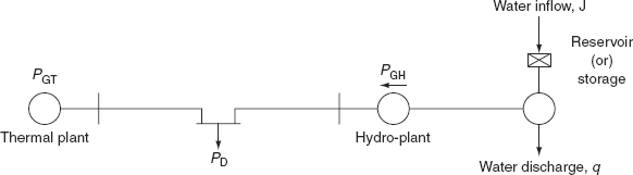
FIG. 6.1 Fundamental hydro-thermal system
The maximum advantage of cheap hydro-power should be taken so that the coal reserves can be conserved and environmental pollution can be minimized. In a hydro-thermal system, the whole or a part of the base load can be supplied by the run-off river hydro-plants and the peak or the remaining load is then met by a proper co-ordination of reservoir-type hydro-plants and thermal plants.
The operating cost of thermal plants is very high and at the same time its capital cost is low when compared with a hydro-electric plant. The operating cost of a hydro-electric plant is low and its capital cost is high such that it has become economical as well as convenient to run both thermal as well as hydro-plants in the same grid.
In the case of thermal plants, the optimal scheduling problem can be completely solved at any desired instant without referring to the operation at other times. It is a static optimization problem.
The operation of a system having both hydro and thermal plants is more complex as hydro-plants have a negligible operating cost but are required to run under the constraint of availability of water for hydro-generation during a given period of time. This problem is the ‘dynamic optimization problem’ where the time factor is to be considered.
The optimal scheduling problem in a hydro-thermal system can be stated as to minimize the fuel cost of thermal plants under the constraint of water availability for hydro-generation over a given period of operation.
Consider a simple hydro-thermal system, shown in Fig. 6.1, which consists of one hydro and one thermal plant supplying power to load connected at the center in between the plants and is referred to as the fundamental system.
To solve the optimization problem in this system, consider the real power generations of two plants PGThermal and PGHydro as control variables. The transmission power loss is expressed in terms of the B coefficient as
6.3 SCHEDULING OF HYDRO-UNITS IN A HYDRO-THERMAL SYSTEM
- In case of hydro-units without thermal units in the system, the problem is simple. The economic scheduling consists of scheduling water release to satisfy the hydraulic constraints and to satisfy the electrical demand.
- Where hydro-thermal systems are predominantly hydro, scheduling may be done by scheduling the system to produce minimum cost for the thermal systems.
- In systems where there is a close balance between hydro and thermal generation and in systems where the hydro-capacity is only a fraction of the total capacity, it is generally desired to schedule generation such that thermal generating costs are minimized.
6.4 CO-ORDINATION OF RUN-OFF RIVER PLANT AND STEAM PLANT
A run-off river hydro-plant operates as the water is available in needed quantities. These plants are provided with a small pondage or reservoir, which makes it possible to meet the hourly variation of load.
The ratio of run-off during the rainy season to the run-off during the dry season may be as large as 100. As such the run-off river plants have very little from capacity. The usefulness of these run-off river plants can be considerably increased if such a plant is properly co-ordinated with a thermal plant. When such co-ordination exists, the hydro-plant may carry the base load upto its installed capacity during the period of high stream flows and the thermal plant may carry the peak load. During the period of lean flow, the thermal plant supplies the base load and the hydro-plant supplies the peak load. Thus, the load met by a thermal plant can be adjusted to conform to the available river flow. This type of co-ordination of a run-off river hydro-plant with a thermal plant results in a greater utilization factor of the river flow and a saving in the amount of fuel consumed in the thermal plant.
6.5 LONG-TERM CO-ORDINATION
Typical long-term co-ordination may be extended from one week to one year or several years. The co-ordination of the operation of reservoir hydro-power plants and steam plants involves the best utilization of available water in terms of the scheduling of water released. In other words, since the operating costs of hydro-plants are very low, hydro-power can be generated at very little incremental cost. In a combined operational system, the generation of thermal power should be displaced by available hydro-power so that maximum decrement production costs will be realized at the steam plant. The long-term scheduling problem involves the long-term forecasting of water availability and the scheduling of reservoir water releases for an interval of time that depends on the reservoir capacities and the chronological load curve of the system. Based on these factors during different times of the year, the hydro and steam plants can be operated as base load plants and peak load plants and vice versa.
For the long-term drawdown schedule, a basic best policy selection must be made. The best policy is that should the water be used under the assumption that it will be replaced at a rate based on the statistically expected rate or should the water be released using a worst-case prediction?
Long-term scheduling is made based on an optimizing policy in view of statistically treated unknowns such as load, hydraulic inflows, and unit availability (i.e., steam and hydro-plants).
The useful techniques employed for this type of scheduling problems include:
- the simulation of an entire long-term operational time period for a given set of operating conditions by using the dynamic programming method,
- composite hydraulic simulation models, and
- statistical production cost models.
For the long-term scheduling of a hydro-thermal system, there should be required generation to meet the requirements of load demand and both hydro and thermal generations should be so scheduled so as to maintain the minimum fuel costs. This requires that the available water should be put to an optimum use.
6.6 SHORT-TERM CO-ORDINATION
The economic system operation of thermal units depends only on the conditions that exist from instant to instant. However, the economic scheduling of combined hydro-thermal systems depends on the conditions existing over the entire operating period.
This type of hydro-thermal scheduling is required for one day or one week, which involves the hour-by-hour scheduling of all available generations on a system to get the minimum production cost for the given time. Such types of scheduling problems, the load, hydraulic inflows, and unit availabilities are assumed to be known.
Here also, the problem is how to supply load, as per the load cycle during the period of operation so that generation by thermal plants will be minimum. This condition will be satisfied when the value of hydro-power generation rather than its amount is a maximum over a certain period. The basic problem is that determining the degree to which the minimized economy of operating the hydro-units at other than the maximum efficiency loading may be tolerated for an increased economy with an increased load or vice versa to result in the lowest total thermal power production costs over the specified operating period.
The factors on which the economic operation of a combined hydro-thermal system depends are as follows:
- Load cycle.
- Incremental fuel costs of thermal power stations.
- Expected water inflow in hydro-power stations.
- Water head that is a function of water storage in hydro-power stations.
- Hydro-power generation.
- Incremental transmission loss (ITL).
The following are the few important methods for short-term hydro-thermal co-ordination:
- Constant hydro-generation method.
- Constant thermal generation method.
- Maximum hydro-efficiency method.
- Kirchmayer’s method.
6.6.1 Constant hydro-generation method
In this method, a scheduled amount of water at a constant head is used such that the hydro-power generation is kept constant throughout the operating period.
6.6.2 Constant thermal generation method
Thermal power generation is kept constant throughout the operating period in such a way that the hydro-power plants use a specified and scheduled amount of water and operate on varying power generation schedules during the operating period.
6.6.3 Maximum hydro-efficiency method
In this method, during peak load periods, the hydro-power plants are operated at their maximum efficiency; during off-peak load periods they operate at an efficiency nearer to their maximum–efficiency with the use of a specified amount of water for hydro-power generation.
Kirchmayer’s method is explained in Section 6.8.
6.7 GENERAL MATHEMATICAL FORMULATION OF LONG-TERM HYDRO-THERMAL SCHEDULING
To mathematically formulate the optimal scheduling problem in a hydro-thermal system, the following assumptions are to be made for a certain period of operation T (a day, a week, or a year):
- The storage of a hydro-reservoir at the beginning and at the end of period of operation T are specified.
- After accounting for the irrigation purpose, water inflow to the reservoir and load demand on the system are known deterministically as functions of time with certainties.
The optimization problem here is to determine the water discharge rate q(t) so as to minimize the cost of thermal generation.
Objective function is
Subject to the following constraints:
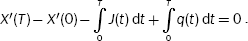
(i) The real power balance equation
PGT(t) + PGH(t) = PL(t) + PD(t) + PD(t)
i.e., PGT(t) + PGH(t) − PL(t) − PD(t) = 0 for t ∈ (0, T) (6.2)
where |
PGT(t) is the real power thermal generation at time ‘t’, |
|
PGH(t) the real power hydro generation at time ‘t’, |
|
PL(t) real power loss at time ‘t’, and |
|
PD(t) the real power demand at time ‘t’. |
(ii) Water availability equation:
where |
X′(t) is the water storage at time ‘t’, |
|
X′(0) the water storage at the beginning of operation time, T, |
|
X′(T) the water storage at the end of operation time, T, |
|
J(t) the water inflow rate, and |
|
q(t) the water discharge rate. |
(iii) Real power hydro-generation
The real power hydro-generation PGH(t) is a function of water storage X′(t) and water discharge rate q(t)
6.7.1 Solution of problem-discretization principle
By the discretization principle, the above problem can be conveniently solved. The optimization interval T is sub-divided into N equal sub-intervals of Δt time length and over each sub-interval, it is assumed that all the variables remain fixed in value.
The same problem can be reformulated as
subject to the following constraints:
(i) Power balance equation
where |
PKGT is the thermal generation in Kth interval, |
|
PKGH the hydro generation in Kth interval, |
|
PKL the transmission power loss in Kth interval and is expressed as |
|
|
|
PKD is the load demand in the Kth interval. |
(ii) Water availability equation:
where X′K is the water storage at the end of interval K, jK the water inflow rate in interval K, and qK the water discharge rate in interval K.
Dividing Equation (6.7) by Δt, it becomes
XK − XK − 1 − jK + qK = 0 for K = 1, 2 … N (6.8)
where ![]() is the water storage in discharge units.
is the water storage in discharge units.
x0 and xN are specified as water storage rates at the beginning and at the end of the optimization interval, respectively.
(iii) The real power hydro-generation in any sub-interval can be written as
PKGH = ho {1 + 0.5 e (XK + XK − 1)} (qK − ρ) (6.9)
where |
ho = 9.81 × 10⁻³ ho′; |
|
ho′ is the basic water head which is corresponding to dead storage, |
|
e the water head correction factor to account for the variation in head with storage, and |
|
ρ the non-effective discharge (due to the need of which a hydro generation can run at no-load condition). |
Equation (6.9) can be obtained as follows:
PKGH = 9.81 × 10⁻³ hKav (qK − ρ) MW
where (qK − ρ) is the effective discharge in m3/s and hKav is the average head in the Kth interval and is given as
where A is the area of cross-section of the reservoir at the given storage
hKav = h′o (1 + 0.5 e(XK + XK−1))
where ![]() , which is tabulated for various storage values
, which is tabulated for various storage values
∴ PKGH = ho {1 + 0.5e(XK + XK − 1)} (qK − ρ
where ho = 9.81 × 10⁻³ h′o.
The optimization problem is mathematically stated for any sub-interval ‘K ’ by the objective function given by Equation (6.5), which is subjected to equation constraints given by Equations (6.6), (6.8), and (6.9).
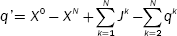
In the above optimization problem, it is convenient to choose water discharges in all sub-intervals except one sub-interval as independent variables and hydro-generations, thermal generations, water storages in all sub-intervals and except water discharge as dependent variables; i.e., independent variables are represented by qK, for K = 2, 3, …, N and for K ≠ 1. Dependent variables are represented by PKGT, PKGH XK, and q1, for K = 1, 2, …, N. [Since the water discharge in one sub-interval is a dependent variable.]
Equation (6.8) can be written for all values of K = 1, 2, …, N:
|
i.e., X1 – X0 – j1 + q1 = 0 |
for K = 1 |
|
X2 – X1 – j2 + q2 = 0 |
for K = 2 |
|
XN – X(N – 1) – jN + qN = 0 |
for k = Nth interval |
By adding the above set of equations, we get

Equation (6.10) is known as the water availability equation.
For K = 2, 3, …, N, there are (N – 1) number of water discharges (q’s), which can be specified as independent variables and the remaining one, i.e., q1, is specified as a dependent variable and it can be determined from Equation (6.10) as
6.7.2 Solution technique
For obtaining a solution to the optimization problem in a hydro-thermal system, a non-linear programming technique in conjunction with the first-order gradient method is used.
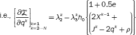
Define the Lagrangian function ![]() by augmenting the objective function (cost function) given by Equation (6.5) with equality constraints given by Equations (6.6), (6.8), and (6.9) through Lagrangian multipliers.
by augmenting the objective function (cost function) given by Equation (6.5) with equality constraints given by Equations (6.6), (6.8), and (6.9) through Lagrangian multipliers.
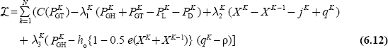
where λ1K,λ2K, and λ3K are the Lagrangian multipliers that are dual variables. These are obtained by taking the partial derivatives of the Lagrangian function with respect to the dependent variables and equating them to zero.
Substituting Equation (6.8) in Equation (6.12) and differentiating the resultant equation with respect to q1, we get
From the above equations, for any sub-interval, the Lagrangian multipliers can be obtained as follows:
- λ1K can be obtained from Equation (6.13),
- λ2K can be obtained from Equation (6.14), and
- λ′2 can be obtained from Equation (6.16) and remaining λ2(K ≠ 1)K can be obtained from Equation (6.15).
The partial derivatives of the Lagrangian function with respect to independent variables give the gradient vector:
For optimality, the gradient vector should be zero ![]() , if there are no inequality constraints on the independent variables, i.e., on control variables (water discharges).
, if there are no inequality constraints on the independent variables, i.e., on control variables (water discharges).
If not we have to find out the new values of control variables that will optimize the objective function, this can be achieved by moving in the negative direction of the gradient vector to a point, where the value of objective function is nearer to the optimal value.
It is an iterative process and this process is repeated till all the components of the gradient vector are closer to zero within a specified tolerance.
6.7.3 Algorithm
Step 1: |
Assume an initial set of independent variables, qK for all sub-intervals except the first sub-interval {i.e., q2, q3 … qN} |
Step 2: |
Obtain the values of dependent variables xK, PKGH,PKGT and q1 using Equations (6.8), (6.9), (6.6), and (6.11), respectively. |
Step 3: |
Obtain the Lagrangian multipliers λK1,λK3 λ2, and λK2 using Equations (6.13), (6.14), (6.16), and (6.15), respectively. |
|
Obtain the gradient vector |
Step 5: |
Obtain new values of control variables using the first-order gradient method, |
where α is a positive scalar, which defines the step length, and having a value depends on the problem on hand, then go to Step 2 and repeat the process.
The inequality constraints of the problem on dependent and independent variables can be handled in the case of an optimal power flow solution. Inequality constraints on independent variables check the Kuhn–Tucker condition (given in optimal power flow, Chapter V). The inequality constraints on dependent variables can be handled by augmenting the objective function through a penalty function.
The above-mentioned solution method can be directly extended to a system having multihydro and multithermal plants.
Drawback: It requires large memory since the independent variables, dependent variables, and gradients need to be stored simultaneously.
A modified technique known as decomposition overcomes the above drawback. In the decomposition technique, optimization is carried out over each sub-interval and a complete cycle of iteration is repeated, if the water availability equation does not check at the end of the cycle.
Example 6.1: A typical hydro-thermal system is shown in Fig. 6.2. For a typical day, the load on the system varies in steps of eight hours each as 9, 12, and 8 MW, respectively. There is no water inflow into the reservoir of the hydro-plant. The initial water storage in the reservoir is 120 m3/s and the final water storage should be 75 m3/s, i.e., the total water available for hydro-generation during the day is 30 m3/s.

FIG. 6.2 Fundamental hydro-thermal system
Basic head is 30 m. Water head correction factor e is given to be 0.004. Assume for simplicity that the reservoir is rectangular so that e does not change with water storage. Let the non-effective water discharge be assumed as 3 m3/s. The fuel cost-curve characteristics of the thermal plant is CT = 0.2 PGT2 +50 PGT + 130 Rs./hr. Find the optimum generation schedule by assuming the transmission losses neglected.
Solution:
Given:
Fuel cost of the thermal plant, CT = 0.2 PGT2 + 50 PGT + 130 Rs./hr
Incremental fuel cost, ![]()
Total time of operation, T |
= 24 hr |
No. of sub-intervals, N |
= 3 |
Duration of each sub-interval, Δt |
= 8 hr |
Initial water storage in reservoir, x′(0) |
= 120 m3/s |
Final water storage, x′(3) |
= 75 m3/s |
Basic water head, h′o |
= 30 m |
Water-head correction factor, e |
= 0.04 |
Non-effective water discharge, ρ |
= 3 m3/s |
Since there are three sub-intervals, (N−1), the number of water discharges of the corresponding sub-intervals can be specified as independent variables and the remaining one is specified as a dependent variable, i.e., the water discharges q2 and q3 are considered as independent variables and dependent variable q1.
Let us assume the initial values to be
q2 = 15 m3/s
q3 = 15 m3/s
for the problem formulation PGH, PGT, x, and q1 are treated as independent variables.
The dependent variable q1 (water discharge in the first sub-interval) can be obtained by Equation (6.11).
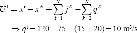
We have the water availability equation,
xK – xk −1 – jK+ qK = 0 for K=1, 2, … N
From the above equation, we have
x1 = xo + j1 – q1 = 120 – 10 = 110 m3/s
x2 = x1 + j2 – q2 = 110 – 15 = 95 m3/s
We know the real power hydro-generation at any interval K by Equation (6.9):
|
PKGH |
= |
ho {1 + 0.5e(xK + xK − 1)}(qk − e) |
|
|
= |
9.81 × 10⁻³ h′o {1 + 0.5e(xK + xK − 1)}(qK − ρ) |
|
P1GH |
= |
9.81 × 10− 3 × 30 {1 + 0.5 × 0.004(x1 + xo) q1 − ρ} |
|
|
= |
9.81 × 10−3 × 30 {1 + 0.5 × 0.004 (110 + 120)} (10 − 3) |
|
|
= |
3.0077 MW |
|
P2GH |
= |
9.81 × 10−3 × 30{1 + 0.5 × 0.004(x2 + x1)q2 − ρ} |
|
|
= |
9.81 × 10−3 × 30 {1 + 0.5 × 0.004 (95 + 110)} (15 − 3) |
|
|
= |
4.9795 MW |
|
P3GH |
= |
9.81 × 10−3 × 30{1 + 0.5 × 0.004(x3 + x2)q2 − ρ} |
|
|
= |
9.81 × 10−3 × 30 {1 + 0.5 × 0.004 (75 + 95)} (20 − 3) |
|
|
= |
6.7041 MW |
The thermal power generations during the sub-intervals are
P1GT = P1D − P1GH = 9 − 3.0077 = 5.9923 MW
P2GT = P2D − P2GH = 12 − 4.9795 = 7.0205 MW
P3GT = P3D − P3GH = 8 − 6.7041 = 1.2959 MW
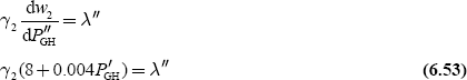
λ1K can be obtained from Equation (6.13):
i.e., 
By neglecting transmission losses, we have
![]()
⇒ λ11 = 0.4P1GT + 50 = 0.4 × 5.9923 + 50 = 52.3969 Rs./MWh
λ12 = 0.4P2GT + 50 = 0.4 × 7.0205 + 50 = 52.8082 Rs./MWh
λ13 = 0.4P3GT + 50 = 0.4 × 1.2959 + 50 = 50.5183 Rs./MWh
From Equation (6.14),
![]()
By neglecting transmission losses, we have
⇒ λ3K = λ1K
∴ λ31 = λ11 = 52.3969 Rs./MWh
λ32 = λ12 = 52.8082 Rs./MWh
λ33 = λ13 = 50.5183 Rs./MWh
From Equation (6.16), we have
![]()
⇒ λ21 = λ21ho {1 + 0.5e(2xo + j1 − 2q1 + ρ)}
= 52.3969 × 9.81 × 10−3 × 30 {1 + 0.5 × 0.004 (2 × 120 − 2 × 10 + 3)
(since j = 0)
= 22.2979 Rs./MWh
From Equation (6.15), we have
For K = 1,
∴ λ22 |
= |
λ22 − λ320.5hoe(q1 − ρ) − λ320.5hoe(q2 − ρ) |
|
= |
22.2979 − {52.3969 × 0.5 × 9.81 × 10−3 × 30 × 0.004(10−3)} |
|
|
− {52.8082 × 0.5 × 9.81 × 10−3 × 30 × 0.004(15−3)} |
|
= |
22.2979 − 0.5889 |
|
= |
21.709 Rs./MWh |
and for K = 2
∴ λ23 |
= |
λ22 − λ22 0.5hoe(q2 − ρ) − λ330.5hoe(q3 − ρ) |
|
= |
21.709 − {52.8082 × 0.5 × 9.81 × 10−3 × 30 × 0.004(15 − 3)} |
|
|
−{50.5183 × 0.5 × 9.81 × 10−3 × 30 × 0.004(20 − 3)} |
|
= |
21.709 − 0.8784 |
|
= |
20.8305 Rs./MWh |
i.e., λ21 |
= |
22.2979 Rs./MWh |
λ22 |
= |
21.709 Rs./MWh |
λ23 |
= |
20.8305 Rs./MWh |
From Equation (6.17), the gradient vector is


If the tolerance value for the gradient vector is 0.1, since for the above iteration, the gradient vector is not zero (≤ 0.1), i.e., the optimality is not satisfied here. Then, for the second iteration, obtain the new values of control variables (qKnew, for K ≠ 1) by using the first-order gradient method as follows:
![]() (∵ α is a positive scalar)
(∵ α is a positive scalar)
![]()
Let us consider α = 0.5,
∴ qnew2 = (q2)1 = 15 − 0.5(0.1685) = 14.9157 m3/s
Similarly, qnew3 = (q3)1 = 15 − 0.5(1.4134) = 19.2933 m3/s
and from Equation (6.11),
|
⇒ q1 |
= xo – x3 – (q2 + q3) (since jK = 0) |
|
q1 |
= 120 – 75 – (14.9157 + 19.2933) |
|
|
= 10.791 m3/s |
To obtain the optimal generation schedule in hydro-thermal co-ordination, the procedure is repeated for the next iteration and checked for a gradient vector. If the gradient vector becomes zero within a specified tolerance, then that will be the optimum generation schedule, otherwise the iterations are to be carried out.
6.8 SOLUTION OF SHORT-TERM HYDRO-THERMAL SCHEDULING PROBLEMS—KIRCHMAYER’S METHOD
In this method, the co-ordination equations are derived in terms of penalty factors of both plants for obtaining the optimum scheduling of a hydro-thermal system and hence it is also known as the penalty factor method of solution of short-term hydro-thermal scheduling problems.
Let |
PGTi be the power generation of ith thermal plant in MW, |
|
PGHj be the power generation of jth hydro-plant in MW, |
|
|
|
wj be the quantity of water used for power generation at jth hydro-plant in m3/s, |
|
|
|
|
|
|
|
λ be the Lagrangian multiplier, |
|
γj be the constant which converts the incremental water rate of hydel plant j into an incremental cost, |
|
n be the total number of plants, |
|
α be the number of thermal plants, |
|
n−α be the number of hydro-plants, and |
|
T be the time interval during which the plant operation is considered. |
Here, the objective is to find the generation of individual plants, both thermal as well as hydel that the generation cost (cost of fuel in thermal) is optimum and at the same time total demand (PD) and losses (PL) are continuously met.
As it is a short-range problem, there will not be any appreciable change in the level of water in the reservoirs during the interval (i.e., the effects of rainfall and evaporation are neglected) and hence the head of water in the reservoir will be assumed to be constant.
Let Kj be the specified quantity of water, which must be utilized within the interval T at each hydro-station j.
Problem formulation
The objective function is to minimize the cost of generation:
i.e.,
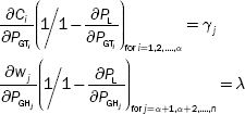
subject to the equality constraints
and
where wj is the turbine discharge in the jth plant in m3/s and Kj the amount of water in m3 utilized during the time period T in the jth hydro-plant.
The coefficient γ must be selected so as to use the specified amount of water during the operating period.
Now, the objective function becomes
Substituting Kj from Equation (6.21) in the above equation, we get
For a particular load demand PD, Equation (6.20) results as
For a particular hydro-plant x, Equation (6.23) can be rewritten as
By rearranging the above equation, we get
From Equation (6.22), the condition for minimization is
The above equation can be written as
For hydro-plant x,

Multiplying the above equation by  ,
,
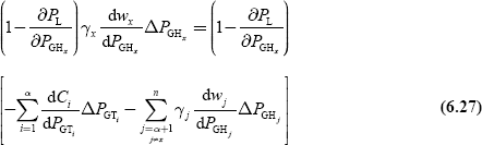
Substitute for 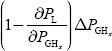 from Equation (6.24) in Equation (6.27), we get
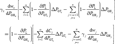
Rewriting the above equation as

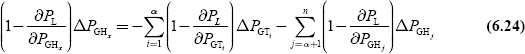
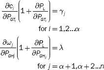
∴ ΔPGTi ≠ 0 and ΔPGHj ≠ 0, Equation (6.28) becomes

and

Equations (6.29) and (6.30) can be written in the form:

and

From Equations (6.31) and (6.32), we have

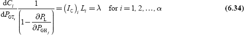
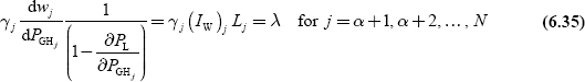
where (IC)i is the incremental fuel cost of the ith thermal plant and (IW)j the incremental water rate of the jth hydro-plant.
Equations (6.34) and (6.35) may be expressed approximately as

where  and
and  are the approximate penalty factors of the ith thermal plant and the jth hydro-plant, respectively.
Equations (6.34) and (6.35) are the co-ordinate equations, which are used to obtain the optimal scheduling of the hydro-thermal system when considering the transmission losses.
In the above equations, the transmission loss PL is expressed as
The power generation of a hydro-plant PGHj is directly proportional to its head and discharge rate wj.
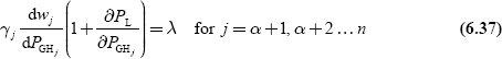
When neglecting the transmission losses, the co-ordination equations become

Example 6.2: A two-plant system having a steam plant near the load center and a hydro-plant at a remote location is shown in Fig. 6.3. The load is 500 MW for 16 hr a day and 350–MW, for 8 hr a day.
The characteristics of the units are
C1 = 120 + 45 PGT + 0.075 P2GT
w2 = 0.6 PGH + 0.00283 P2GH m3/s
Loss coefficient, B22 = 0.001 MW−1
Find the generation schedule, daily water used by the hydro-plant, and daily operating cost of the thermal plant for γj = 85.5 Rs./m3-hr.
Solution:
Given: C1 = 120 + 45 PGT + 0.075 P2GT
Co-ordination equation for thermal unit is
![]() 45 + 0.15 PGT + 0.075 P2GT
45 + 0.15 PGT + 0.075 P2GT

FIG. 6.3 A typical two-plant hydro-thermal system
For the hydro-unit, the co-ordination equation is
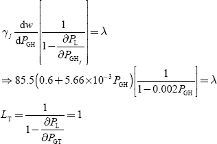
Since the load is nearer to the thermal plant, the transmission loss is only due to the hydro-plant and therefore BTT = BTH = BHT = 0:

Power balance equation, PGT + PGH = PD + PL and the condition for optimal scheduling is
When PD = 500 MW
0.15 PGT + 45 = 85.5(0.6 + 5.66 × 10⁻³PGH) ![]()
(0.15 PGT + 45) (1 − 0.002 PGH) = 85.5 (0.6 + 5.66 × 10⁻³PGH)
0.15 PGT + 45 − 3 × 10⁻⁴ PGTPGH − 0.09 PGT = 51.3 + 0.48393 PGH
0.57393 PGH − 0.15 PGT + 3 × 10⁻⁴ PGT PGH + 6.3 = 0 (6.39)
and
PGT + PGH = 400 + 0.001 P2GT
PGT = 400 + 0.001 P2GT − PGH (6.40)
Substituting Equation (6.40) in Equation (6.39), we get
0.57393 PGH − 0.15(400 + 0.001 P2GH − PGH) + 3 × 10⁻⁴
PGH (400 + 0.001 P2GH − PGH ) + 6.3 = 0
By solving the above equation, we get
PGH = 81.876 MW
By substituting the PGH value in Equation (6.40), we get
PGT = 424.8 MW
PL = 6.70367 MW
When PD = 350 MW
Equation (6.40) can be modified as
PGT = 350 + 0.001 P2GH − PGH (6.41)
Substituting Equation (6.41) in Equation (6.39), we get
0.57393 PGH − 0.15(350 + 0.001 P2GH − PGH) + 3 × 10⁻⁴
PGH (350 + 0.001 P2GH − PGH) + 6.3 = 0
By solving the above equation, we get
PGH = 58.5851 MW
By substituting the PGH value in Equation (6.41), we get
PGT = 294.847 MW
PL = 3.43221 MW
Daily water used by the hydro-plant
|
w |
|
0.6 PGH + 0.00283 P2GH m3/s |
|
|
= |
Daily water quantity used for a 500 MW load for 16 hr + daily water quantity used for a 350 MW load for 8 hr |
|
|
= |
{[0.6 × 81.876 + 0.00283 × (81.876)2] × 14 + [0.6 × 58.586 + 0.00283 × (58.586)2] × 8} × 3600 |
|
|
= |
5.21449 × 10⁶ m3 |
Daily operating cost of the thermal plant is:
|
C1 |
= |
(120 + 45 PGT + 0.075 P2GT) |
|
|
= |
Operating cost of the thermal plant for meeting the 500 MW load for 16 hr + operating cost of the thermal plant for meeting the 350 MW load for 8 hr |
|
|
= |
[120 + 45 × 424.8 + 0.075(424.8)2] × 16 + [120 + 45 × 294.85 + 0.075(424.8)2] × 8 |
|
|
= |
Rs. 6,83,589.96 per day |
Example 6.3: A two-plant system that has a hydro-plant near the load center and a steam plant at a remote location is shown in Fig. 6.4. The load is 400 MW for 14 hr a day and 200 MW, for 10 hr a day.
The characteristics of the units are
C1 = 150 + 60 PGT + 0.1 P2GT Rs/hr
w2 = 0.8 PGH + 0.000333 P2GH m3/s

FIG. 6.4 A typical two-plant hydro-thermal system
Loss coefficient, B22 = 0.001 MW−1
Find the generation schedule, daily water used by the hydro-plant, and the daily operating cost of a thermal plant for γj = 77.5 Rs./m3hr.
Solution:
Equations for thermal and hydro-plants are

Since the load is nearer to the hydro-plant, the transmission loss is only due to the thermal plant and therefore BHH = BTH = BHT = 0:
When PD = 400 MW
The power balance equation is
|
PGT + PGH |
= |
PD + PL |
|
|
= |
400 + 0.001 P2GT |
|
PGH |
= |
400 + 0.001 P2GT − PGT (6.42) |
The condition for optimal scheduling problem is

0.2 PGT + 60 = 77.5 (0.8 + 6.6 × 10⁻⁴ PGH) (1 − 0.002 PGT)
0.2 PGT + 60 = 62 + 0.051615 PGH − 0.124 PGT − 1.032 × 10⁻⁴ PGH PGT
0.2 PGT + 0.124 PGT + 1.032 × 10⁻⁴ PGHPGT − 0.0516 PGH − 2 = 0 (6.43)
Substituting PGH from Equation (6.42) in Equation (6.43), we get
0.2 PGT + 0. 124 PGT + 1.032 × 10⁻⁴ PGT (400 + 0.001 P2GT − PGT)
− 0.0516(400 + 0.001 P2GT − PGT) − 2 = 0
By solving the above equation, we get
PGT = 55.4 MW
By substituting the PGT value in Equation (6.42), we get
PGH = 347.66 MW
PL = 3.069 MW
When PD = 200 MW
From Equation (6.42), the power balance equation becomes
PGH = 200 0.001 P2GT − PGT (6.44)
Substituting PGH from Equation (6.44) in Equation (6.43), we get
0.2 PGT + 0.124 PGT + 1.032 × 10⁻⁴ PGT (200 + 0.001 P2GH − PGT)
− 0.0516 (200 + 0.001 P2GT − PGT) − 2 = 0
By solving the above equation, we get
PGT = 31.575 MW
By substituting the PGH value in Equation (6.44), we get
PGH = 169.421 MW
PL = 0.9969 MW
Daily operating cost of the thermal plant
|
C1 |
= |
150 + 60 PGT + 0.1 P2GT |
|
|
= |
Daily operating cost of the thermal plant for meeting a 400 MW load for 14 hr + daily operating cost of the thermal plant for meeting a 200 MW load for 10 hr |
|
|
= |
[150 + 60 × 55.4 + 0.1 × (55.4)2] × 14 + [150 + 60 × 31.575 + 0.1 × (31.575)2] × 10 |
|
|
= |
Rs. 74,374.80 |
Daily operating cost of the hydro-plant
|
w |
= |
0.8 PGH + 0.000333 P2GH m3/s |
|
|
= |
Daily water quantity used for the 400 MW load for 14 hr + daily water quantity used for the 200 MW load for 10 hr |
|
|
= |
{[0.8 × 347.66 + 0.000333 × (347.66)2] × 14 + [0.8 × 169.421 + 0.000333 × (169.421)2] × 10 × 3600 |
|
|
= |
21.2696 × 10⁶ m3 |
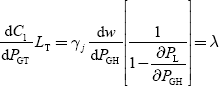
Example 6.4: A two-plant system that has a thermal station near the load center and a hydro-power station at a remote location is shown in Fig. 6.5.
The characteristics of both stations are
C1 = (26 + 0.045PGT)PGT Rs./hr
w2 = (7 + 0.004PGH)PGH m3/s
and γ2 = Rs. 4 × 10⁻⁴/m3
The transmission loss coefficient, B22 = 0.0025 MW−1.
Determine the power generation at each station and the power received by the load
when λ = 65 Rs./MWh.
Solution:
Here, n = 2
Transmission loss,
Since the load is near the thermal station, the power flow is from the hydro-station only; therefore, B12 = B11 = 0:
For the thermal power station, the co-ordination equation is

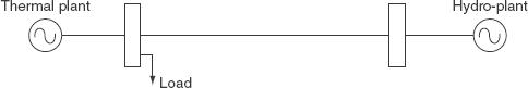
FIG. 6.5 Two-plant system
For a hydro-power station, the co-ordination equation is

By solving the above equation, we get
PGH = 199.99 MW
Transmission loss, PL = B22 P2GH = 0.0025(199.99)2 = 99.993 MW
Therefore, the power received by the load, PD = PGT + PGH − PL = 433.33 + 622.38 − 193.68 = 533.327 MW.
Example 6.5: For the system of Example 6.4, if the load is 750 MW for 14 hr a day and 500 MW for 10 hr on the same day, find the generation schedule, daily water used by the hydro-plant, and the daily operating cost of thermal power.
Solution:
When load, PD = 750 MW
The power balance equation, PGT + PGH = PD + PL
= 750 + 0.0025 P2GH
PGT = 750 + 0.0025 P2GH − PGH (6.45)
The condition for optimality is

(26 + 0.09 PGT) (1 − 5 × 10− 3PGH) = 28 × 10−4 + 32 × 10−7 PGH (6.46)
Substituting PGT from Equation (6.45) in Equation (6.46), we get
[26 + 0.09 (750 + 0.0025 P2GH − PGH)](1 − 5 × 10− 3 PGH) = 28 × 10−4 + 32 × 10−7 PGH
− 1.125 × 10⁻⁶ P3GH + 6.75 × 10⁻⁴P2GH − 0.5574 PGH + 25.9922 = 0
By solving the above equation, we get
PGH = 200 MW
Substituting the PGH value in Equation (6.45), we get
PGT = 650 MW and PL = 100 MW
When load, PD = 400 MW
Equation (6.45) can be modified as
PGT = 400 + 0.0022 P2GH − PGH (6.47)
Substituting the above equation in Equation (6.46), we get
[26 + 0.09 (400 + 0.0025 P2GH − PGH)](1 − 5 × 10− 3 PGH) = 28 × 10−4 + 32 × 10−7 PGH
− 1.125 × 10⁻⁶ P3GH + 6.75 × 10⁻⁴P2GH − 0.3999 PGH + 61.9972 = 0
By solving the above equation, we get
PGH = 200 MW
Substituting the PGH value in Equation (6.47), we get
PGT = 300 MW and PL = 100 MW
Daily operating cost of the hydro-plant
|
w2 |
= |
(7 + 0.004PGH) PGH m3/s |
|
|
= |
Daily water quantity used for a 750 MW load for 14 hr + daily water quantity used for a 400 MW load for 10 hr |
|
|
= |
{[7 × 200 + 0.004 × (200)2] × 14 + [7 × 200 + 0.004 × (200)2] × 10} × 3600 |
|
|
= |
134.784 × 10⁶ m3 |
Daily operating cost of the thermal plant
|
C1 |
= |
(26 + 0.045PGT) PGT Rs./hr |
|
|
= |
Daily operating cost of a thermal plant for meeting a 750 MW load for 14 hr + daily operating cost of thermal plant for meeting a 400 MW load for 10 hr |
|
|
= |
[26 × 650 + 0.045 × (650)2] × 14 + [26 × 300 + 0.045 × (300)2] × 10 |
|
|
= |
Rs. 6,21,275 |
Example 6.6: A load is feeded by two plants, one is thermal and the other is a hydro-plant. The load is located near the thermal power plant as shown in Fig. 6.6. The characteristics of the two plants are as follows:
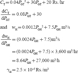
CT = 0.04PGT2 + 30PGT + 20 Rs./hr
wH = 0.0012 PGH2 + 7.5PGH m3/s
γH = 2.5 × 10⁻⁵ Rs./m3

FIG. 6.6 Two-plant system
The transmission loss co-efficient is B22 = 0.0015 MW−1. Determine the power generation of both thermal and hydro-plants, the load connected when λ = 45 Rs./MWh.
Solution:
Given:
Transmission loss,

The load is located near the thermal plants; hence, the power flow to the load is only from the hydro-plant:
i.e., B11 = B12 = 0
∴ PL = B22 PG22 = B22 PGH2 = 0.0015 PGH2
The incremental transmission loss of the thermal plant is
![]()
Penalty factor of the thermal plant, 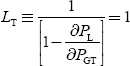
The incremental transmission loss of the hydro-plant is
Penalty factor of the hydro-plant, 
The condition for hydro-thermal co-ordination is

and ![]()
or (0.000216 PGH + 0.675) |
= |
(1 − 0.003 PGH)45 |
0.135216 PGH |
= |
44.325 |
∴ PGH |
= |
327.809 MW |
Transmission loss, PL = B22 PGH2 = 0.0015(327.809)2 = 161.188 MW
The load connected, PD = PGT + PGH − PL = 187.5 + 327.809 − 161.188 = 354.121 MW
Example 6.7: For Example 6.6, determine the daily water used by the hydro-plant and the daily operating cost of the thermal plant with the load connected for totally 24 hr.
Solution:
From Example 6.6,
The load connected, PD |
= 354.121 MW |
Generation of the thermal plant, PGT |
= 187.5 MW |
Generation of the hydro-plant, PGH |
= 327.809 MW |
The daily water used is
|
wH |
= |
0.0012 PGH2 + 7.5 PGH m3/s |
|
|
= |
[0.0012 PGH2 + 7.5 PGH] × 3,600 m3/hr |
|
|
= |
[0.0012 PGH2 + 7.5 PGH] × 3,600 × 24 m3/day |
Substituting the value of PGH = 327.809 MW in the above equation, we have
|
wH |
= |
[0.0012(327.809)2 + 7.5 × 327.809] × 3,600 × 24 |
|
|
= |
223.56 × 10⁶ m3 |
Daily operating cost of the thermal plant |
= |
(0.04 PGT2 + 30 PGT + 20) Rs./h |
|
= |
Rs. [0.04(187.5)2 + 30 (187.5) + 20] × 24 |
|
= |
Rs.1,69,230 |
Example 6.8: In a two-plant operation system, the hydro-plant operates for 8 hr during each day and the steam plant operates throughout the day. The characteristics of the steam and hydro-plants are
CT = 0.025PGT2 + 14PGT + 12 Rs./hr
wH = 0.002PGH2 + 28PGH m3/s
When both plants are running, the power flow from the steam plant to the load is 190 MW and the total quantity of water used for the hydro-plant operation during 8 hr is 220 × 106 m3.
Determine the generation of a hydro-plant and cost of water used. Neglect the transmission losses.
Solution:
The cost of the thermal plant is
CT = (0.025 PGT2 + 14PGT + 12) Rs./hr
The incremental fuel cost of the thermal plant is
![]()
and for the hydro-plant, wH = (0.002PGH2 + 28PGH) m3/s
The incremental water flow is
![]()
For hydro-thermal scheduling, the optimal condition is
(since losses are neglected, LT = 1)
Power flow to the load from the thermal plant, PGT = 190 MW (given). By substituting the value of PGT = 190 MW in the above equation, we get
λ = 0.05(190) + 14 = 23.5 Rs./MWh
The total quantity of water used during a one-hour operation is
|
wH |
= 0.0012 PGH2 + 7.5PGH m3/s |
|
|
= [0.0012 PGH2 + 7.5PGH] × 3,600 m3/hr |
For an 8-hr operation, the quantity of water used is
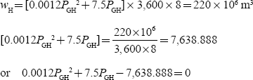

Let the cost of water be γH Rs./hr/m3/s.
From Equation (6.48)

Example 6.9: A two-plant system with no transmission loss shown in Fig. 6.7(a) is to supply a load shown in Fig. 6.7(b).
The data of the system are as follows:
C1 = (32 + 0.03PGT)PGT
w2 = (8 + 0.004PGH)PGH m3/s
The maximum capacity of the hydro-plant and the steam plant are 450 and 250 MW, respectively. Determine the generating schedule of the system so that 150.3478 million m3 water is used during the 24-hr period.

FIG. 6.7 (a) Two-plant system; (b) daily load curve
Solution:
(i) Constant hydro-generation
If PGH is the hydro-power in MW generated in 24 hr, then we have
|
(8 + 0.004 PGH)PGH × 24 × 60 × 60 |
= |
150.3478 × 10⁶ |
|
8 PGH + 0.004 P2GH |
= |
1,740.136 |
|
0.004 P2GH + 8 PGH − 1,740.136 |
= |
0 |
By solving the above equation, we get
PGH = 197.929 MW
During the peak load of 600 MW
Hydro-generation, PGH = 197.929 MW
Thermal generation, PGT = 600 - PGH = 600 - 197.929 = 402.071 MW
During off-peak load of 400 MW
Hydro-generation, PGH = 197.929 MW
Thermal generation, PGT = 400 - PGH = 400 - 197.929 = 402.071 MW
The running cost of a steam plant for 24 hr is
|
C1 |
= |
(32 + 0.03PGT)PGT × 12/at 600 MW + (32 + 0.03PGT)PGT × 12/at 400 MW |
|
|
= |
(32 + 0.03 × 402.071) 402.071 × 12 + (32 + 0.03 × 202.071) 202.071 × 12 |
|
|
= |
Rs. 3,04,888.288 |
(ii) Constant thermal generation
If PGH is the hydro-power during the peak load period
(PGH – 200) is the hydro-power during the off-peak load period
Given w2 = (8 + 0.004PGH)PGH m3/s
{(8 + 0.004PGH)PGH + [8 + 0.004(PGH − 200)](PGH − 200)} × 12 × 3,600 = 150.3478 × 10⁶
After simplification, we get
8 × 10 − 3 PGH2 + 14.4PGH – 4,920.273 = 0
∴ PGH = 93.74793 MW
The generation scheduling is given as follows:
| Hydro | Thermal (PD – PGH) | |
|---|---|---|
Peak (600) |
293.75 MW |
306.25 MW |
Off-peak (400) |
93.75 MW |
306.25 MW |
The steam plant operating cost for 24 hr is
|
C1 |
= |
(32 + 0.03PGT)PGT |
|
|
= |
(32 + 0.03 × 306.25) 306.25 × 12 + (32 + 0.03 × 306.25) 306.25 × 12 |
|
|
= |
Rs. 3,02,728.125 |
(iii) Equal incremental plant costs
Let P′GT and P′GH be the steam generation and hydro-generation during peak loads, P″GT and P″GH the steam generation and hydro-generation during off-peak loads, respectively.
For peak load conditions:

The value of λ′ should be so chosen as to make
For off-peak periods:
The value of λ″ should be chosen so as to make
For the whole operating period, γ2 should be chosen so as to use the same value of water, i.e., 150.3478 million m3 during the 24-hr period.
{(8 + 0.004 P′GH )P′GH +(8 + 0.004 P″GH )P″GH } × 12 × 3,600 = 150.3478 × 10⁶ (6.55)
All the above equations can be solved by a hit-and-trail or an iterative method:
|
P′GT |
= |
276.362 MW, P′GH = 323.638MW |
|
λ′ |
= |
48.58172 Rs./MWh |
|
|
|
− (8 + 0.004 × 323.638) × 323.638 + 3,480.273= (8 + 0004 P‴GH )P″GH |
|
8 P′GH |
= |
+ 0.004 P″2GH = 472.2 |
By solving the above equation, we get
|
P″GH + 57.38 MW P″GT |
= |
342.62 MW |
|
λ″ |
= |
52.5572 Rs. /MWh |
|
γ2 |
= |
6.2131 Rs./hr/m3/s |
The thermal operating cost
|
C1 |
= |
(32 + 0.03 PGT)PGT |
|
|
= |
(32 + 0.03 × 276.362) × 276.362 × 12 + (32 + 0.03 × 342.62) × 342.62 × 12 |
|
|
= |
Rs. 3,07,444.279 |
(iv) Maximum hydro-efficiency method
Let it be assumed that the maximum efficiency of a hydro-unit occurs at 275 MW.
Therefore, the hydro-power plant supply is 275 MW during the peak load. The amount of water used during peak load hours:
|
w2 | = (8 + 0.004PGH)PGH m3/s |
| = (8 + 0.004 × 275) × 275 × 12 × 3,600 = 108.108 × 10⁶ |
Water available for off-peak hydro-generation:
= total water available – water available at peak load
= 150.34 × 10⁶ − 108.108 × 106 = 42.2398 × 10⁶ m3
The real power generation of a hydro-plant PGH during off-peak hours is found by using
(8 + 0.004PGH) PGH × 12 × 3600 = 4,22,39,800
0.004PGH2 + 8PGH – 977.77 = 0
PGH(Off-peak load) = 115.5461 MW
The generation scheduling is given as follows:
| Hydro | Thermal (PD – PGH) | |
|---|---|---|
Peak (600) |
273 MW |
325 MW |
Off-peak (400) |
115.546 MW |
284.4539 MW |
The daily operating cost of a thermal plant
|
C1 |
= |
(32 + 0.03PGT)PGT |
|
|
= |
(32 + 0.03 × 325) 325 × 12 + (32 + 0.03 × 284.4539) 284.4539 × 12 |
|
|
= |
Rs. 12,43,023.55 |
Example 6.10: A thermal station and a hydro-station supply an area jointly. The hydro-station is run 16 hr daily and the thermal station is run through 24 hr. The incremental fuel cost characteristics of the thermal plant are
CT = 6 + 12 PGT + 0.04PGT2 Rs./hr
If the load on the thermal station, when both plants are in operation, is 350 MW, the incremental water rate of a hydro-power plant ![]() . The total quantity of water utilized during a 16-hr operation of the hydro-plant is 450 million m3. Find the generation of the hydro-plant and cost of water use. Assume that the total load on the hydro-plant is constant for the 16-hr period.
. The total quantity of water utilized during a 16-hr operation of the hydro-plant is 450 million m3. Find the generation of the hydro-plant and cost of water use. Assume that the total load on the hydro-plant is constant for the 16-hr period.
Solution:
Given: CT = 6 + 12PGT + 0.04PGT2
![]()
PGT = 350 MW (given)
∴ 12 + 0.08 × 350 = λ
λ = 40Rs./MWh
The total quantity of water used during 16 hr of operation of a hydro-plant is
(28 + 0.03PGH)PGH × 16 × 3, 600 = 450 × 106
0.03PGH2 + 28PGH = 7,812.5
0.03PGH2 + 28PGH – 7,812.5 = 0
By solving the above equation, we get
PGH = 224.849 MW
If the cost of water used is γ, then we have
γ (28 + 0.03PGH) = λ
γ (28 + 0.03 × 224.849) = 40
∴ γ = 1.15122 Rs./hr/m3/s
6.9 ADVANTAGES OF OPERATION OF HYDRO-THERMAL COMBINATIONS
The following advantages are obtained by operation combination of hydro-thermal power plants.
6.9.1 Flexibility
The power system reliability and security can be obtained by the combined operation of hydro and thermal units. It provides the reserve capacity to meet the random phenomena of forced outage of units and unexpected load implied on a system.
Thermal plants require an appreciable time for starting and for being put into service. Hydro-plants can be started and put into operation very quickly with lower operating costs. Hence, it is required to operate hydro-plants economically as base-load plants as well as peak load plants. Hydro-plants are most preferable to operate as peak load plants such that their operation improves the flexibility of the system operation and makes the thermal plant operation easier.
6.9.2 Greater economy
The run-off river hydro-plants would generally meet the entire or part of the base loads, and thermal plants should be set up to increase the firm capacity of the system. The remaining power demand can be met by a combination of reservoir-type hydro-plants, thermal plants, and nuclear plants. In every power system, a certain ratio of hydro-power to total power demand will result in a minimum overall cost of supply.
6.9.3 Security of supply
Water availability must depend on the season. It is high during the rainy season and may be reduced due to the occurrence of draught during longer plants. Problems arise in the thermal power plant operation due to transportation of coal, unavailability of labor, etc. It is found that the forced outages of hydro-plants are few compared to those in thermal plants.
The above facts suggested the operation of hydro-thermal systems to maintain the reliability and security of supply to the consumers.
6.9.4 Better energy conservation
During heavy run-off periods, the generation of hydro-power is more, which results in the conservation of fossil fuels. During draught periods, more steam power has to be generated such that the availability of water needs the minimum needs like drinking and agricultural events.
6.9.5 Reserve capacity maintenance
For the operation of a power system, it is necessary that every system has some certain reserve capacity to meet the forced outages and unexpected load demands. By the combined operation of hydro and thermal plants, the reserve capacity maintenance is reduced.
Example 6.11: MATLAB program on hydro-thermal scheduling without inflow and without loss. Find the optimum generation for a hydro-thermal system for a typical day, wherein load varies in three steps of 8 hr each as 15, 25, and 8 MW, respectively. There is no water inflow into the reservoir of the hydro-plant. The initial water storage in the reservoir is 180 m3/s and the final water storage should be 100 m3/s. The basic head is 35 m and the water-head correction factor e is 0.005. Assume for simplicity that the reservoir is rectangular so that ρ does not change with water storage. Let the non-effective water discharge be assumed as 4 m3/s. The incremental fuel cost (IFC) of the thermal power plant is ![]() . Further transmission losses may be neglected.
. Further transmission losses may be neglected.
PROGRAM IS UNDER THE FILE NAME hydrothermal.m
clc;
clear;
load =[15;25;8]; %load in MW
time =[8;8;8]; time of each load
ni=length(load(:,1);
x(1)=180;
x(ni+1)=100;
h0=35;
e=0.005;
ro=4;
ifc=[2.0 25.0];
delt=time(1);
alpha=0.5;
%assuming in initial discharges
q(2)=20;
q(3)=22;
maxgrad=1;
iter=0;
while(maxgrad>0.1)
iter=iter+1;
sumq=0;
for I=2:ni
sumq=sumq+q(i);
end
q(1)=x(1)−x(ni+1)−sumq;
for I=2:ni
x(i)=x(i−1)−q(i−1); %water storage before ith interval
end
for i=1:ni
pd(i)=load(i,1);
pgh(i)= 9.81*0.001*h0*(1+0.5*e*(x(i)+x(i+1)))*(q(i)−ro);
if pgh(i)>pd(i)
pgh(i)=pd(i);
pgt(i)=0;
else
pgt(i)=pd(i)−pgh(i);
end
lambda1(i)=ifc(1,1)*pgt(i)+ifc(1,2);
lambda3(i)=lambda1(i);%since losses are neglected
if i==1
lambda2(i)=lambda3(i)*9.81*0.001*h0*(1+0.5*e*(2*x(i)−
2*q(i)+ro));
else
lambda2(i)=lambda2(i−1)−0.5*9.81*0.001*h0*e*(lambda3
(i−1)*(q(i−1)−ro)+lambda3(i)*(q(i)−ro));
end
if i~=1
grad(i)=lambda2(i)−lambda3(i)*9.81*0.001*h0*(1+0.5*e*(2*x
(i)−2*q(i)+ro));
end
end
maxgrad=(max(abs(grad)));
for i=2:ni
q(i)=q(i)−alpha*(grad(i));
end
end
pgh
pgt
iter
RESULTS:
pgh = 12.4706 |
21.8178 |
5.4672 |
pgt = 2.5294 |
3.1822 |
2.5328 |
netPG = 15 |
25 |
8 |
iter = 15 |
|
|
Example 6.12: MATLAB program on hydro-thermal scheduling with inflow and without losses. Find the optimum generation for a hydro-thermal system for a typical day, wherein load varies in three steps of 8 hr each as 15, 25, and 8 MW, respectively. There is water inflow into the reservoir of the hydro-plant in three intervals of 2, 4, and 3 m3/s. The initial water storage in the reservoir is 180 m3/s and the final water storage should be 100 m3/s. The basic head is 35–m and the water-head correction factor e is 0.005. Assume for simplicity that the reservoir is rectangular so that ρ does not change with water storage. Let the non-effective water discharge be assumed as 4 m3/s. The IFC of the thermal power plant is ![]() Further transmission losses may be neglected.
Further transmission losses may be neglected.
PROGRAM IS UNDER THE FILE NAME hydrothermalinflow.m
clc;
clear;
load=[15;25;8]; %load in MW
time=[8;8;8]; %time of each load
ni=length(load(:,1));
x(1)=180;
x(ni + 1)=100;
h0=35;
e=0.005;
ro=4;
ifc=[2.0 25.0];
delt=time(1);
alpha=0.5;
J=[2;4;3];
%assuming initial discharges
q(2)=20;
q(3)=22;
maxgrad=1;
iter=0;
while(maxgrad>0.1)
iter=iter + 1;
sumq=0;
sumj=0;
for i=2:ni
sumq=sumq + q(i);
end
for i=1:ni
sumj=sumj + J(i,1);
end
q(1)=x(1)−x(ni+1)−sumq + sumj;
for i=2:ni
x(i)=x(i−1)−q(i−1) + J(i,1); %water storage before ith
interval
end
for i=1:ni
pd(i)=load(i,1);
pgh(i)=9.81*0.001*h0*(1 + 0.5*e*(x(i) + x(i + 1)))*(q(i)−ro);
if pgh(i)>pd(i)
pgh(i)=pd(i);
pgt(i)=0;
else
pgt(i)=pd(i)−pgh(i);
end
lambda1(i)=ifc(1,1)*pgt(i) + ifc(1,2);
lambda3(i)=lambda1(i); %since losses are neglected
if i=1
lambda2(i)=lambda3(i)*9.81*0.001*h0*(1 + 0.5*e*(2*x(i)−
2*q(i) + J(i,1) + ro));
else
lambda2(i)=lambda2(i−1)−0.5*9.81*0.001*h0*e*(lambda3
(i−1)*(q(i−1)−ro) + lambda3(i)*(q(i)−ro));
end
if i~=1
grad(i)=lambda2(i)−
lambda3(i)*9.81*0.001*h0*(1 + 0.5*e*(2*x(i)−
2*q(i) + J(i,1) + ro));
end
end
maxgrad=max(abs(grad));
for i=2:ni
q(i)=q(i)−alpha*(grad(i));
end
end
pgh
pgt
iter
RESULTS:
pgh = 14.0553 |
23.6463 |
7.3583 |
pgt = 0.9447 |
1.3537 |
0.6417 |
netPG = 15 |
25 |
8 |
iter = 15 |
|
|
Example 6.13: MATLAB program on hydro-thermal scheduling without inflow and with losses. Find the optimum generation for a hydro-thermal system for a typical day, wherein load varies in three steps of 8 hr each as 15, 25, and 8 MW, respectively. There is no water inflow into the reservoir of the hydro-plant. The initial water storage in the reservoir is 180 m3/s and the final water storage should be 100 m3/s. The basic head is 35 m and the water-head correction factor e is 0.005. Assume for simplicity that the reservoir is rectangular so that ρ does not change with water storage. Let the non-effective water discharge be assumed as 4 m3/s. The IFC of the thermal power plant is ![]() . Further transmission losses are considered and are taken as follows:
. Further transmission losses are considered and are taken as follows: ![]() .
.
PROGRAM IS UNDER THE FILE NAME hydrothermalloss.m
clc;
clear;
load=[15;25;8]; %load in MW
time=[8;8;8]; %time of each load
ni=length(load(:,1));
x(1)=180;
x(ni + 1)=100;
h0=35;
e=0.005;
ro=4;
ifc=[2.0 25.0];
delt=time(1);
alpha=0.5;
dpl=0.5;
%assuming initial discharges
q(2)=20;
q(3)=22;
maxgrad=1;
iter==0;
while(maxgrad>0.1)
iter=iter + 1;
sumq=0;
for i=2:ni
sumq=sumq + q(i);
end
q(1)=x(1)−x(ni + 1)−sumq;
for i=2:ni
x(i)=x(i−1)−q(i−1); %water storage before ith interval
end
for i=1:ni
pd(i)=load(i,1);
pgh(i)=9.81*0.001*h0*(1 + 0.5*e*(x(i) + x(i + 1)))*(q(i)−ro);
if pgh(i)>pd(i)
pgh(i)=pd(i);
pgt(i)=0;
else
pgt(i)=pd(i)−pgh(i);
end
lambda1(i)=(ifc(1,1)*pgt(i) + ifc(1,2))/(1−dpl);
lambda3(i)=lambda1(i)*(1−dpl);
if i==1
lambda2(i)=lambda3(i)*9.81*0.001*h0*(1 + 0.5*e*(2*x(i)−
2*q(i) + ro));
else
lambda2(i)=lambda2(i−1)−0.5*9.81*0.001*h0*e*(lambda3
(i−1)*(q(i−1)−ro) + lambda3(i)*(q(i)−ro));
end
if i~=1
grad(i)=lambda2(i)−
lambda3(i)*9.81*0.001*h0*(1 + 0.5*e*(2*x(i)−2*q(i) + ro));
end
end
maxgrad=(max(abs(grad)));
for i=2:ni
q(i)=q(i)−alpha*(grad(i));
end
end
pgh
pgt
iter
grad
RESULTS:
pgh = 12.4706 |
21.8178 |
5.4672 |
pgt = 2.5294 |
3.1822 |
2.5328 |
grad = 0 |
−0.0765 |
0.0826 |
netPG = 15 |
25 |
8 |
iter = 15 |
|
|
Example 6.14: MATLAB program on hydro-thermal scheduling with inflow and with losses. Find the optimum generation for a hydro-thermal system for a typical day, wherein load varies in three steps of 8 hr each as 15, 25 and 8 MW, respectively. There is water inflow into the reservoir of the hydro-plant in three intervals of 2, 4, 3 m3/s. The initial water storage in the reservoir is 180 m3/s and the final water storage should be 100 m3/s. The basic head is 35 m and the water-head correction factor e is 0.005. Assume for simplicity that the reservoir is rectangular so that ρ does not change with water storage. Let the non-effective water discharge be assumed as 4 m3/s. The IFC of the thermal power plant is ![]() . Further transmission losses are considered and are taken as follows:
. Further transmission losses are considered and are taken as follows: ![]()
PROGRAM IS UNDER THE FILE NAME hydrothermalinflowloss.m
clc;
clear;
load=[15;25;8]; %load in MW
time=[8;8;8]; %time of each load
ni=length(load(:,1));
x(1)=180;
x(ni + 1)=100;
h0=35;
e=0.005;
ro=4;
ifc=[2.0 25.0];
delt=time(1);
alpha=0.5;
J=[2;4;3];
dpl=0.15;
%assuming initial discharges
q(2)=20;
q(3)=22;
maxgrad=1;
iter=0;
while(maxgrad>0.1)
iter=iter + 1;
sumq=0;
sumj=0;
for i=2:ni
sumq=sumq + q(i);
end
for i=1:ni
sumj=sumj + J(i,1);
end
q(1)=x(1)−x(ni + 1)−sumq + sumj;
for i=2:ni
| x(i)=x(i−1)−q(i−1) + J(i,1); | %water storage before ith |
| interval |
end
for i=1:ni
pd(i)=load(i,1);
pgh(i)=9.81*0.001*h0*(1 + 0.5*e*(x(i) + x(i + 1)))*(q(i)−ro);
if pgh(i)>pd(i)
pgh(i)=pd(i);
pgt(i)=0;
else
pgt(i)=pd(i)−pgh(i);
end
lambda1(i)=(ifc(1,1)*pgt(i) + ifc(1,2))/(1−dpl);
lambda3(i)=lambda1(i)*(1−dpl);
if i=1
lambda2(i)=lambda3(i)*9.81*0.001*h0*(1 + 0.5*e*(2*x(i)−
2*q(i) + J(i,1) + ro));
else
lambda2(i)=lambda2(i−1)−0.5*9.81*0.001*h0*e*(lambda3
(i−1)*(q(i−1)−ro) + lambda3(i)*(q(i)−ro));
end
if i~=1
grad(i)=lambda2(i)−
lambda3(i)*9.81*0.001*h0*(1 + 0.5*e*(2*x(i)−
2*q(i) + J(i,1) + ro));
end
end
maxgrad=max(abs(grad));
for i=2:ni
q(i)=q(i)−alpha*(grad(i));
end
end
pgh
pgt
iter
RESULTS:
pgh = 14.0553 |
23.6463 |
7.3583 |
pgt = 0.9447 |
1.3537 |
0.6417 |
netPG = 15 |
25 |
8 |
iter = 15 |
|
|
KEY NOTES
- The optimal scheduling problem in the case of thermal plants can be completely solved at any desired instant without referring to the operation at other times. It is a static optimization problem.
- The optimal scheduling problem in the hydro-thermal system is a dynamic optimization problem where the time factor is to be considered.
- The optimal scheduling problem in a hydro-thermal system can be stated as minimizing the fuel cost of thermal plants under the constraint of water availability for hydro-generation over a given period of operation.
- The methods of hydro-thermal co-ordination are:
- Constant hydro-generation method.
- Constant thermal generation method.
- Maximum hydro-efficiency method.
- Kirchmayer’s method.
- Constant hydro-generation method—A scheduled amount of water at a constant head is used such that the hydro-power generation is kept constant throughout the operating period.
- Constant thermal generation method—Thermal power generation is kept constant throughout the operating period in such a way that the hydro-power plants use a specified and scheduled amount of water and operate on varying power generation schedule during the operating period.
- Maximum hydro-efficiency method—During peak-load periods, the hydro-power plants are operated at their maximum efficiency; during off-peak load periods, they operate at an efficiency nearer to their maximum efficiency with the use of a specified amount of water for hydro-power generation.
- Kirchmayer’s method—The co-ordination equations are derived in terms of penalty factors of both plants for obtaining the optimum scheduling of the hydro-thermal system and hence it is also known as the penalty factor method of solution of short-term hydro-thermal scheduling problems.
- Long-term hydro-thermal scheduling problems can be solved by the discretization principle.
- In the long-term hydro-thermal scheduling problem, it is convenient to choose water discharges in all sub-intervals except one sub-interval as independent variables and hydro-generations, thermal generations, water storages in all sub-intervals, and excepted water discharge as dependent variables,
i.e., Independent variables are represented by qK, for K = 2, 3,…,N
≠ 1
Dependent variables are represented by PKGH, PKGT, XK, and q1, for K = 1,2,…,N. [Since the water discharge in one sub-interval is a dependent variable.]
- For optimality of long-term hydro-thermal scheduling, the gradient vector should be zero, i.e.,
 .
.
SHORT QUESTIONS AND ANSWERS
- Why is the optimal scheduling problem in the case of thermal plants referred to as a static optimization problem?
Optimal scheduling problem can be completely solved at any desired instant without referring to the operation at other times.
- The optimization problem in the case of a hydro-thermal system is referred to as a dynamic problem. Why is it so?
The operation of the system having hydro and thermal plants have negligible operation costs but is required under the constraint of water availability for hydro-generation over a given period of time.
- What is the statement of optimization problem of hydro-thermal system?
Minimize the fuel cost of thermal plants under the constraint of water availability for hydro-generation over a given period of time.
- In the optimal scheduling problem of a hydro-thermal system, which variables are considered as control variables?
Thermal and hydro-power generations (PGT and PGH).
- Fast-changing loads can be effectively met by which type of plants?
Hydro-plants.
- Generally, which type of plants are more suitable to operate as base-load and peak load plants?
Thermal plants are suited for base-load plants and hydro-plants are suited for peak load plants.
- Whole or part of the base load can be supplied by which type of hydro-plants?
Run-off river type.
- The peak load or remaining base load is met by which type of plants?
A proper co-ordination of reservoir-type hydro-plants and thermal plants.
- In the optimal scheduling problem of a hydro-thermal system, what parameters are assumed to be known as the function of time with certainty?
Water inflow to the reservoir and load demand.
- What is the mathematical statement of the optimization problem in the hydro-thermal system?
Determine the water discharge rate q(t) so as to minimize the cost of thermal generation.
- Write the objective function expression of hydro-thermal scheduling problem.

- Write the constraint equations of the hydro-thermal scheduling problem.
PGT(t) + PGH(t) − PL(t) − PD(t) = 0
for t ∈ (O,T)—Real power balance equation

—PGH(t) = (X‴ (t), q(t))
- By which principle can the optimal scheduling problem of a hydro-thermal system be solved?
Discretization principle.
- Write the expression for real power hydro-generation in any sub-interval ‘K’?
PKGH = ho {1 + 0.5e (XK + X K − 1)} (qK − ρ)
- Define the terms of the above real power hydro-generation.
PKGH = ho {1 + 0.5e (XK + X K − 1)} (qK − ρ)
where h0 = 9.81 × 10⁻³ h01, ho1 is the basic water head that corresponds to dead storage, e the water-head correction factor to account for the variation in head with water storage, Xk the water storage at interval k, qk the water discharge at interval k, and ρ the non-effective discharge.
- In the optimal scheduling problem of a hydro-thermal system, which variables are used to choose as independent variables?
Water discharges in all sub-intervals except one sub-interval:
i.e., ekk ≠1, for q2, q3 ⋯ qN
where k = 2, 3 … N (k is sub-interval).
- Which parameters are used as dependent variables?
Thermal, hydro-generations, water storages at all sub-intervals, and water discharge at excepted sub-intervals are used as dependent variables,
i.e., PGTk, PGHk Xk, and q1
- In solving the optimal scheduling problem of a hydro-thermal system, for ‘N’ sub-intervals (i.e., k = 1, 2, …, N), N−1 number of water discharges q’s can be specified as independent variables except one sub-interval. Write the expression for water discharge in the excepted sub-interval, which is taken as a dependant variable.
- Which technique is used to obtain the solution to the optimization problem of the hydro-thermal system?
A non-linear programming technique in conjunction with a first-order negative gradient method is used to obtain the solution to the optimization problem.
- Write the expression for a Lagrangian function obtained by augmenting the objective function with constraint equations in the case of a hydro-thermal scheduling problem.

- What is the gradient vector?
The partial derivatives of the Lagrangian function with respect to independent variables are
- What is the condition for optimality in the case of a hydro-thermal scheduling problem?
The gradient vector should be zero:

- The condition for optimality in a hydro-thermal scheduling problem is that the gradient vector should be zero. If this condition is violated, how will we obtain the optimal solution?
Find the new values of control variables, which will optimize the objective function. This can be achieved by moving in the negative direction of the gradient vector to a point where the value of the objective function is nearer to an optimal value.
- For a system with a multihydro and a multithermal plant, the non-linear programming technique in conjunction with the first-order gradient method is also directly applied. However, what is the drawback?
It requires large memory since the independent and dependant variables, and gradients need to be stored simultaneously.
- By which method can the drawback of the non-linear programming technique be overcome when applied to a multihydro and multithermal plant system and what is its procedure?
By the method of decomposition technique. In this technique, the optimization is carried out over each sub-interval and a complete cycle of iteration is replaced, if the water availability equation does not check at the end of the cycle.
- For short-range scheduling of a hydro-thermal plant, which method is useful?
Kirchmayer’s method or the penalty factor method is useful for short-range scheduling.
- What is Kirchmayer’s method of obtaining the optimum scheduling of a hydro-thermal system?
In Kirchmayer’s method or the penalty factor method, the co-ordination equations are derived in terms of penalty factors of both hydro and thermal plants.
- What is the condition for optimality in a hydro-thermal scheduling problem when considering transmission losses?
where i represents the thermal plant and j represents the hydro-plant.
- What is the meaning of the terms
 and
and  ?
?
 is the incremental cost of the i th thermal plant and
 is the incremental water rate of the jth hydro-plant.
 - What is short-term hydro-thermal co-ordination?
Short-term hydro-thermal co-ordination is done for a fixed quantity of water to be used in a certain period (i.e., 24 hr).
- What are the scheduling methods for short-term hydro-thermal co-ordination?
- Constant hydro-generation method.
- Constant steam generation method.
- Maximum hydro-efficiency method.
- Equal incremental production costs and solution of co-ordination equations (Kirchmayer’s method).
- What is the significance of the co-efficient γj?
γj represents the incremental water rates into incremental costs which must be so selected as to use the desired amount of water during the operating period.
- Write the condition for optimality in the problem of a short range hydro-thermal system according to Kirchmayer’s method when neglecting transmission losses.

- What is the significance of terms
 and
and  ?
?
 is the penalty factor of the ith thermal plant and
 is the penalty factor of the jth hydro-plant
These terms are very much useful in getting the optimality in a hydro-thermal scheduling problem, which is solved by Kirchmayer’s method.
- Write the condition for optimality in an optimal scheduling problem of a short range hydro-thermal system with approximate penalty factors.
MULTIPLE-CHOICE QUESTIONS
- When compared to a hydro-electric plant, the operating cost of the thermal plant is very _____ and its capital cost is _____.
- High, low.
- High, high.
- Low, low.
- Low, high.
- When compared to a thermal plant, the operating cost and capital cost of a hydro-electric plant are:
- High and low.
- Low and high.
- Both high.
- Both low.
- The optimal scheduling problem in the case of thermal plants is:
- Static optimization problem.
- Dynamic optimization problem.
- Static as well as dynamic optimization problem.
- Either static or dynamic optimization problem.
- The operation of the system having hydro and thermal plants is more complex. In this case, the optimal scheduling problem is:
- Static optimization problem.
- Dynamic optimization problem.
- Static as well as dynamic optimization problem.
- Either static or dynamic optimization problem.
- The optimal scheduling problem in the case of a thermal plant can be completely solved at any desired instant:
- With reference to the operation at other times.
- Without reference to the operation at other times.
- Case (a) or case (b) that depends on the size of the plant.
- None of these.
- The time factor is considered in solving the optimization problem of _____.
- Hydro plants.
- Thermal plants.
- Hydro-thermal plants.
- None of these.
- The objective function to the optimization problem in a hydro-thermal system becomes:
- Minimize the fuel cost of thermal plants.
- Minimize the time of operation.
- Maximize the water availability for hydro-generation.
- All of these.
- The optimal scheduling problem of a hydro-thermal system is solved under the constraint of:
- Fuel cost of thermal plants for thermal generation.
- Time of operation of the entire system.
- Water availability for hydro-generation over a given period.
- Availability of coal for thermal generation over a given period.
- To solve the optimization problem in a hydro-thermal system, which of the following variables are considered as control variables?
- PD thermal and PG hydro.
- QD thermal and QD hydro.
- PG thermal and PD hydro.
- PG thermal and PG hydro.
- In which system is the generation scheduled generally such that the operating costs of thermal generation are minimized?
- Systems where there is a close balance between hydro and thermal generation.
- Systems where the hydro-capacity is only a fraction of the total capacity.
- Both (a) and (b).
- None of these.
- Thermal plants are more suitable to operate as _____ plants leaving hydro-plants to operate as _____ plants.
- Base load, base load.
- Peak load, peak load.
- Peak load, base load.
- Base load, peak load.
- In hydro-thermal systems, the whole are part of the base load that can be supplied by:
- Run-off river-type hydro-plants.
- Reservoir-type hydro-plants.
- Thermal plants.
- Reservoir-type hydro-plants and thermal plants with proper co-ordination.
- In a hydro-thermal system, the peak load can be met by:
- Run-off river-type hydro-plants.
- Reservoir-type hydro-plants.
- Thermal plants.
- Reservoir-type hydro-plants and thermal plants with proper co-ordination.
- For an optimal scheduling problem, it is assumed, which parameter is known deterministically as a function of time?
- Water inflow to the reservoir.
- Power generation.
- Load demand.
- Both (a) and (c).
- In a hydro-thermal system, the optimization problem is stated as determining _____ so as to minimize the cost of thermal generation.
- Load demand (PD).
- Water storage (X).
- Water discharge rate (q(t)).
- Water inflow rate (J(t)).
- Which of the following equations is considered as a constraint to the optimization problem of a hydro-thermal system?
- Real power balance equation.
- Water availability equation.
- Real power hydro-generation as a function of water storage.
- All of these.
- The water availability equation is:
- PGH(t) + PGH(t) − PL(t) − PD(t) = 0, t∈(0,T).
- PGH(t) = f(X′(t), q(t)).
- None of these.
- In the optimization problem of a hydro-thermal system, the constraint real power hydro-generation is a function of:
- Water inflow rate (J(t)).
- Water storage (X).
- Water discharge rate (q(t))
- (i) and (ii).
- (ii) and (iii).
- (i) and (iii).
- None of these.
- The optimization scheduling problem of a hydro-thermal system can be conveniently solved by _____ principle.
- Dependence.
- Discretization.
- Dividing.
- None of these.
- In the discretization principle, the real power hydro-generation at any sub-interval ‘k’ can be expressed as:
- PKGH = ho {1 + 0.5e (Xk − 1 + Xk)} (qk − ρ)
- PKGH = ho {1 − 0.5e (Xk − 1 + Xk)} (qk − ρ)
- PKGH = ho {1 + 0.5e (Xk − 1 + Xk)} (qk − ρ)
- PKGH = ho {1 + 0.5e (Xk − 1 + Xk − 1)} (qk − ρ)
- In the optimization problem of a hydro-thermal system, which of the following are closed as independent variables?
- Water storages in all sub-intervals except one sub-interval.
- Water inflows in all sub-intervals except one sub-interval.
- Water discharges in all sub-intervals except one sub-interval.
- Hydro and thermal generations, water storages at all sub-intervals, and water discharge at one sub-interval.
- In the optimal scheduling problem of a hydro-thermal system, which of the following are closed as dependent variables?
- Water storages in all sub-intervals except one sub-interval.
- Water inflows in all sub-intervals except one sub-interval.
- Water discharges in all sub-intervals except one sub-interval.
- Hydro and thermal generations, water storages at all sub-intervals, and water discharge at one sub-interval.
- To obtain the solution to the optimization problem of a hydro-thermal system, which of the following technique is used?
- Non-linear programming technique in conjunction with the first-order gradient method.
- Linear programming technique in conjunction with the first-order gradient method.
- Non-linear programming technique in conjunction with the multiple-order gradient method.
- Linear programming technique in conjunction with the multiple-order gradient method.
- In a hydro-thermal system for optimality, the condition is:
- Gradient vector should be zero.
- Gradient vector should be positive.
- Gradient vector should be negative.
- None of these.
- For multihydro and multithermal plants, the optimization problem can be solved by a modified technique, which is known as:
- Discretization technique.
- Decomposition technique.
- Decoupled technique.
- None of these.
- In Kirchmayer’s method of solution of optimization problem in a hydro-thermal system, the co-ordination equations are derived in terms of _____ of both plants.
- Power generations.
- Power demands.
- Penalty factors.
- All of these.
- γj is used as a constant, in an optimization problem of a hydro-thermal system, which converts:
- Fuel cost of a thermal plant into an incremental fuel cost.
- Incremental water rate of a hydro-plant into an incremental cost.
- Incremental water inflow rate into an incremental discharge rate.
- None of these.
- The power generation of a hydro-plant PGH is directly proportional to:
- Plant head.
- Water discharge ωj.
- Both (a) and (b).
- None of these.
- The main advantages of the operation of a hydro-thermal system are:
- Greater economy.
- Security of supply and flexibility.
- Better energy conservation.
- Reduction in reserve capacity maintenance.
Regarding the above statement, which is correct?
- (i) and (ii).
- (ii) and (iii).
- all except (iii).
- All of these.
- The co-ordination equations used to obtain the optimal scheduling of a hydro-thermal system when considering transmission losses are:

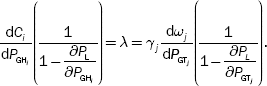
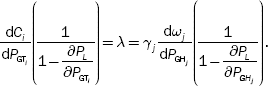
- None of these.
- As far as possible, hydro-plants are used for base-load operation since:
- Their capital cost is high.
- Their operation is easy.
- Their capital cost is low.
- Their efficiency is low.
- A thermal plant gives minimum cost per unit of energy generated when used as a _____ plant.
- Peak load.
- Base-load plant.
- Simultaneously as base-load and peak load plant.
- None of these.
- In the combined operation of steam plant and run-off river plants, the sites of hydro and steam plants can be found with the help of _____.
- Demand curve.
- Input–output curve.
- Load curve.
- Chronological load curve.
- Long-term hydro-thermal co-ordination can be done by:
- Plotting the basic rule curve.
- Plotting no spill-rule curve.
- Plotting the full reservoir storage curve.
- All of these.
- _____ hydro-thermal co-ordination is done for the available water and is to be used in a given period (24 hr).
- Long-term.
- Short-term.
- Both (a) and (b).
- None of these.
- Hydro-thermal co-ordination is necessary only in countries with:
- Ample coal resources.
- Ample water resources.
- Both (a) and (b).
- None of these.
- In short-term hydro-thermal co-ordination,
- No spill-rule curve is used.
- Spill-rule curve is used.
- Here no rule curve is used due to constraints.
- None of these.
- The units of incremental water rate are:
- m3/s-MW.
- m3-s/MW.
- m-s/MW.
- m2-s/MW.
- Hydro-generation is a function of:
- Water head.
- Water discharge.
- Water inflow.
- Both (a) and (b).
- In the long-term hydro-thermal co-ordination,
- Basic rule curve is plotted.
- No spill curve.
- No full reservoir storage curve.
- All of these.
- In the combined operation of a steam and a run-off river plant, the sizes of hydro and steam plants can be obtained with the help of:
- Load curve.
- Demand curve.
- Chronological load curve.
- None of these.
REVIEW QUESTIONS
- Explain the hydro-thermal co-ordination and its importance.
- Describe the types of hydro-thermal co-ordination.
- What are the factors on which economic operation of a combined hydro-thermal system depends?
- What are the important methods of hydro-thermal co-ordination? Explain them in brief.
- Explain the mathematical formulation of long-term hydro-thermal scheduling.
- Explain the solution method of long-term hydro-thermal scheduling by discretization principle.
- Develop an algorithm for the solution of long-term hydro-thermal scheduling problem.
- Derive the condition for optimality of short-term hydro-thermal scheduling problem.
- What are the advantages of hydro-thermal plants combinations?
PROBLEMS
- The system shown in Fig. 6.8(a) is to supply a load shown in Fig. 6.8(b). The data of the system are as follows:
CT = (16 + 0.01PGT)PGTRs./hr
w2 = (4 + 0.0035PGH)PGHm3/s
The maximum capacity of a hydro-plant and a steam plant are 400 and 270 MW, respectively. Determine the generating schedule of the system so that 130.426 million m3 water is used during the 24-hr period.
- A thermal station and a hydro-station supply an area jointly. The hydro-station is run 12 hr daily and the thermal station is run throughout 24 hr. The incremental fuel cost characteristic of the thermal plant is
CT = 3 + 5PGT + 0.02PGT Rs/hr
If the load on the thermal station, when both plants are in operation, is 250 MW, the incremental water rate of the hydro-power plant is
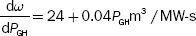
The total quantity of water utilized during the 12-hr operation of a hydro-plant is 450 million m3. Find the generation of the hydro-plant and the cost of water used. Assume that the total load on the hydro-plant is constant for the 12-hr period.
- A two-plant system that has a thermal station near the load center and a hydro-power station at a remote location is shown in Fig. 6.9.
The characteristics of both stations are:
CT = (20 + 0.03PGT)PGTRs./hr
w2 = (8 + 0.002PGH)PGHm3/s
and γ2 = Rs. 5 × 10⁻⁴/m3
The transmission loss co-efficient, B22 = 0.0005.
- if the load is 700 MW for 15-hr a day and 500 MW for 9 hr on the same day, find the generation schedule, daily water used by hydro-plant, and the daily operating cost of the thermal power.
- Determine the power generation at each station and the power received by the load when λ = 50 Rs./MWh.
- A two-plant system that has a hydro-station near the load center and a thermal power station at a remote location is shown in Fig. 6.10.
The characteristics of both stations are
CT = (20 + 0.03PGT)PGTRs./hr
w2 = (8 + 0.002PGH)PGHm3/s
and γ2 = Rs. 5.5/m3
The transmission loss co-efficient, B22 = 0.0005.
- If the load is 700 MW for 15 hr a day and 500 MW for 9 hr on the same day, find the generation schedule, daily water used by the hydro-plant, and the daily operating cost of thermal power.
- Determine the power generation at each station and the power received by the load when λ = 50 Rs. /MWh.
FIG. 6.8 Illustration for Problem 1; (a) two-plant system; (b) daily load curve
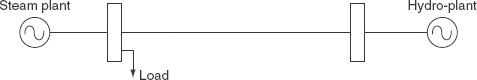
FIG. 6.9 Two-plant system
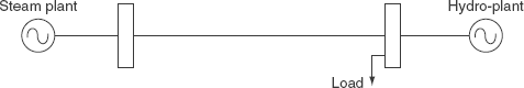
FIG. 6.10 Two-plant system