
5
Optimal Power-Flow Problem—Solution Technique
OBJECTIVES
After reading this chapter, you should be able to:
- know the optimal power flow problem concept
- study the major steps for optimal power flow solution techniques
- formulate the mathematical modeling for optimal power flow problem with and without inequality constraints
- develop algorithms for optimal power flow problems with and without inequality constraints
5.1 INTRODUCTION
The problem of optimizing the performance of a power system network is formulated as a general optimization problem. It is required to state from which aspect the performance of the power system network is optimized.
In optimization problem, the objective function becomes ‘to minimize the overall cost of generation in economic scheduling and unit commitment problem’:
- It is based on allocating the total load on a station among various units in an optimal way with cases being taken into consideration in a load-scheduling problem.
- It is based on allocating the total load on the system among the various generating stations.
The optimal power flow problem:
- refers to the load flow that gives maximum system security by minimizing the overloads,
- aims at minimum operating cost and minimum losses,
- should be based on operational constraints, and
- is a static optimization problem with the cost function as a scalar objective function.
The solution technique for an optimal power flow problem was first proposed by Dommel and Tinney and has following three major steps:
- It is based on the load flow solution by the Newton–Raphson (N–R) method.
- A first-order gradient method consists of an algorithm that adjusts the gradient for minimizing the objective function.
- Use of penalty functions to account for inequality constraints on dependent variables.
The optimization problem of minimizing the instantaneous operating costs in terms of real and reactive-power flows is studied in this unit.
The optimal power flow problem without considering constraints, i.e., unconstrained optimal power flow problem, is first studied and then the optimal power flow problem with inequality constraints is studied. The inequality constraints are introduced first on control variables and then on dependent variables.
5.2 OPTIMAL POWER-FLOW PROBLEM WITHOUT INEQUALITY CONSTRAINTS
The primary objective of the optimal power flow solution is to minimize the overall cost of generation. This is represented by an objective function (or) cost function as:
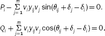
subject to power (load) flow constraints:
and
where Vi = |Vi|∠δi is the voltage at bus ‘i’, Vj = |Vj|∠δj the voltage at bus ‘j’, Yij = |Yij|∠θij the mutual admittance between the i th and j th buses, Pi the specified real-power at bus i, Qi the specified reactive power at bus i, the net real power injected into the system at the i th bus, Pi = PGi – PDi, and the net reactive power injected into the system at the i th bus, Qi = QGi – QDi.
For load buses (or) P–Q buses, P and Q are specified and hence Equations (5.2) and (5.3) form the equality constraints.
For P–V buses, P and |V| are specified as the function of some vectors and are represented as:
f(x, y) = 0
where x is a vector of dependent variables and is represented as

and y is a vector of independent variables and is represented as
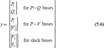
Out of these independent variables (Equation (5.6)), certain variables are chosen as control variables, which are to be varied to yield an optimal value of the objective function. The remaining independent variables are called fixed or disturbance or uncontrollable parameters.
Let ‘u’ be the vector of control variables and ‘p’ the vector of fixed or disturbance variables.
Hence, the vector of independent variables can be represented as the combination of vector of control variables ‘u’ and vector of fixed or disturbance or uncontrollable variables ‘p’ and is expressed as
The choice of ‘u’ and ‘p’ depends on what aspect of power system is to be optimized. The control parameters may be:
- voltage magnitude at P–V buses,
- PGi at generator buses with controllable power,
- slack bus voltage and regulating transformer tap setting as additional control variables, and
- in the case of buses with reactive-power control, QGi is taken as a control variable.
Now, the optimal power flow problem can be stated as
subject to equality constraints:
Define the corresponding Lagrangian function ![]() by augmenting the equality constraint to the objective function through a Lagrangian multiplier λ as
by augmenting the equality constraint to the objective function through a Lagrangian multiplier λ as
where λ is a vector of the Lagrangian multiplier of suitable dimension and is the same as that of equality constraint, f (x, u, p).
The necessary conditions for an optimal solution are as follows:
Equation (5.13) is the same as equality constraints, and the expressions for ![]() and
and ![]() are not very involved.
are not very involved.
Consider the general load flow problem of the N–R method by considering a set of ‘n’ non-linear algebraic equations,
fi(x1, x2 … xn) = 0 for i = 1, 2 … n (5.14)
Let x10, x20, … xn0 be the initial values.
and let ∆x10, ∆x20, … ∆xn0 be the corrections, which on being added to the initial guess, give an actual solution:
∴ fi(x10 + Δx10, + x20 + Δx20, …, xn0 + Δxn0) = 0 for i = 1, 2 … n (5.15)
By expanding these equations according to Taylor’s series around the initial guess, we get
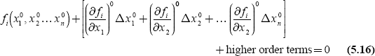
where ![]() are the derivatives of fi with respect to x1, x2 … xn evaluated at (x10, x20, … xn0).
are the derivatives of fi with respect to x1, x2 … xn evaluated at (x10, x20, … xn0).
Neglecting higher order terms, we can write Equation (5.16) in a matrix form as

or in a vector matrix form as
where J 0 is known as the Jacobian matrix and is obtained by differentiating the function vector ‘f ’ with respect to ‘x’ and evaluating it at x 0.
By comparing Equations (5.11), (5.12), and (5.13) with Equations (5.17) and (5.18), it is observed that ![]() is the Jacobian matrix and the partial derivatives of equality constraints with respect to dependent variables are obtained as Jacobian elements in a load flow solution.
is the Jacobian matrix and the partial derivatives of equality constraints with respect to dependent variables are obtained as Jacobian elements in a load flow solution.
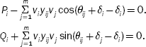
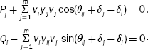
The equality constraints are basically the power flow equations, i.e., real and reactive-power flow equations:
![]() equality constraints for P–Q bus
equality constraints for P–Q bus
Pi is the equality constraint for P–V bus
‘x’ is the dependent variable like |Vi|, δi
Then, ![]() may be expressed as partial derivatives of
may be expressed as partial derivatives of ![]()
The Equations (5.11), (5.12), and (5.13) are non-linear algebraic equations and can be solved iteratively by employing a simple technique that is a ‘gradient method’ and is also called the steepest descent method.
The basic technique employed in the steepest descent method is to adjust the control parameters ‘u’ so as to move from one feasible solution point to a new feasible solution point in the direction of the steepest descent (or negative gradient). Here, the starting point of feasible solution is one where a set of values ‘x’ (i.e., dependent variables) satisfies Equation (5.13) for given ‘u’ and ‘p’. The new feasible solution point refers to a location where the lower objective function is achieved.
These moves are to be repeated in the direction of negative gradient till minimum value is reached. Hence, this method of obtaining a solution to non-linear algebraic is also called the negative gradient method.
5.2.1 Algorithm for computational procedure
The algorithm for obtaining an optimal solution by the steepest descent method is given below:
Step 1: Make an initial guess for control variables (u0).
Step 2: Find the feasible load flow solution by the N–R method. The N–R method is an iterative method and the solution does not satisfy the constraint equation (5.13). Hence, to satisfy Equation (5.12), ‘x’ is improved as follows:
xr + 1 = xr + Δx
∆x is obtained by solving the set of linear equations of the Jacobian matrix of Equation (5.18) as given below:
f (xr + Δx, y) = f (xr, y) + ![]() (xr, y) Δx = 0
(xr, y) Δx = 0
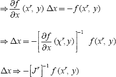
The final results of Step-2 provide a feasible solution of ‘x’ and the Jacobian matrix.
Step 3: Solve Equation (5.11) for λ and it is obtained as
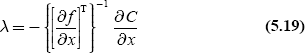
Step 4: Substitute λ from Equation (5.19) into Equation (5.12) and calculate the gradient:
For computing the gradient, the Jacobian matrix, ![]() , is already known from Step 2.
, is already known from Step 2.
Step 5: If the gradient ∇![]() is nearly zero within the specified tolerance, the optimal solution is obtained. Otherwise,
is nearly zero within the specified tolerance, the optimal solution is obtained. Otherwise,
Step 6: Find a new set of control variables as
where Δu = − α∇![]() . (5.22)
. (5.22)
Here, ∆u is a step in the negative direction of the gradient.
The parameter α is a positive scalar, which controls the step i’s (size of steps), and the choice of α is very important.
Too small a value of α guarantees the convergence but slows down its rate. Too high a value of it causes oscillations around the optimal solution. Several methods are suggested for determining the best value of α for a given problem and for an optimum choice of step size.
α is a problem-dependent constant. Experience and proper judgment are necessary in choosing a value of it. Steps 1, 2, and 5 are repeated for a new value of ‘u’ till an optimal solution is reached.
5.3 OPTIMAL POWER-FLOW PROBLEM WITH INEQUALITY CONSTRAINTS
5.3.1 Inequality constraints on control variables
In Section 5.2, the unconstrained optimal power flow problem and the computational procedure for obtaining the optimal solution are discussed. Now, in this section, the inequality constraints are introduced on control variables, and then the method of obtaining a solution to the optimal power flow problem is discussed.
The permissible values of control variables, in fact, are always constrained, such that
For example, if the real power or reactive-power generation are taken as control variables, then inequality constraints become
|
PGi (min) ≤ PGi ≤ PGi (max) |
|
|
QGi (min) ≤ QGi ≤ QGi (max) |
(5.24) |
In finding the optimal power flow solution, Step 6 of the algorithm of Section 5.2.1 gives the change in control variable as
Δu = − α∇![]()
where ![]() and the new control variable, unew = uold + ∆u.
and the new control variable, unew = uold + ∆u.
This new value of control variable must be checked whether it violates the inequality constraints on the control variable or not:
i.e., ui(min) ≤ ui(new) ≤ ui(max)
If the correction ∆u causes to exceed one of the limits, ‘ui’ is set equal to the corresponding limit, i.e., the new value of ui is determined as
otherwise set ui(new) = ui(old) + ∆ui
After a control variable reaches any of the limits, its component in the gradient should continue to be computed in later iteration, as the variable may come within limits at some later stages.
The optimality condition under inequality constraints can be rewritten as Kuhn–Tucker conditions given below:
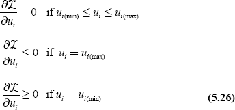
Therefore, now, in Step 5 of the algorithm of Section 5.2.1, the gradient vector has to satisfy the optimality condition given by Equation (5.26).
5.3.2 Inequality constraints on dependent variables—penalty function method
In this section, the optimal solution to an optimal power flow problem will be obtained with the introduction of inequality constraints on dependent variables and penalties for their violation.
The inequality constraints on dependent variables specified in terms of upper and lower limits are
where x is a vector of dependent variables.
For example, if the bus voltage magnitude |Vi| is taken as a dependent variable, the inequality constraint becomes
The above-mentioned inequality constraints can be handled conveniently by a method known as the penalty function method. In this method, the objective function is augmented by penalties for the violations of inequality constraints. Due to this augmented objective function, the solution lies sufficiently close to the constraint limits when the violations of these limits have taken place. The penalty function method, in this case, is valid since these constraints are seldom rigid limits in the strict sense but are, in fact, soft limits (e.g., |V| ≤ 1.0 on a P–Q bus really means |V| should not exceed 1.0 too much and |V| = 1.01 may still be permissible).
When inequality constraints are violated, the objective function can be modified by augmenting penalties as
where ωj is the penalty introduced for each of the violated inequality constraints.
A suitable penalty function is defined as
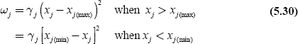
where γj is called a penalty factor since it controls the degree of penalty and is a real positive number.
A plot of the penalty function, which is proposed, is shown in Fig. 5.1. The plot clearly indicates how the rigid limits are replaced by soft limits. The necessary optimality conditions:
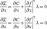
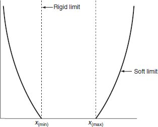
FIG. 5.1 Penalty function
would now be modified as given below, while the condition of Equation (5.13), i.e., load flow equations, remains unchanged:
In the above equations, the vector ![]() can be calculated from the penalty function ωj.
can be calculated from the penalty function ωj.
The vector ![]() can be obtained from Equation (5.30) and would contain one non-zero term corresponding to dependent variable xj .
can be obtained from Equation (5.30) and would contain one non-zero term corresponding to dependent variable xj .
The vector ![]() , since the penalty functions on dependent variables are independent of control variables.
, since the penalty functions on dependent variables are independent of control variables.
If we choose a higher value for γj, the penalty function ωj can be made steeper so that the solution lies closer to the rigid limits, but the convergence becomes poorer. In normal practice, it is required to start with a lower value of γj and then increase it during the optimization process if the solution violates constraints above a certain tolerance limit.
It is concluded that the solution to optimal power flow problem can be achieved by superimposing the N–R method of load flow on the optimal power flow problem with respect to relevant inequality constraints. These solutions are often required for system planning and operation.
KEY NOTES
- The optimal power flow problem:
- refers to load flow, which gives maximum system security by minimizing the overloads,
- aims at minimum operating cost and minimum losses,
- should be based on operational constraints, and
- is a static optimization problem with cost function as the scalar objective function.
- The solution technique for optimal power flow problem proposed by Dommel and Tinney has the following three major steps:
- it is based on the load flow solution by the N–R method.
- a first-order gradient method consists of an algorithm that adjusts the gradient for minimizing the objective function.
- use of penalty functions to account for inequality constraints on dependent variables.
- For P–V buses, P and |V| are specified as functions of some vectors and are represented as f (x, y) = 0 where x is a vector of dependent variables and y is a vector of independent variables.
- The vector of independent variables can be represented as the combination of vector of control variables ‘u’ and vector of fixed or disturbance or uncontrollable variables ‘p’ and is expressed as

- The control parameters are:
- voltage magnitude at P–V buses,
- PGi at generator buses with controllable power,
- slack bus voltage and regulating transformer tap setting as additional control variables, and
- in the case of buses with reactive-power control, QGi is taken as control variable.
- Optimal power flow problem can be stated as
min C = C(x, u)
subject to equality constraints:
f(x, u, p) = 0
SHORT QUESTIONS AND ANSWERS
- The solution technique proposed by Dommel and Tinney for the optimal power flow problem is based on three major steps. What are they?
- Load flow solution by N–R method.
- A first-order gradient method.
- Use of penalty functions to account for inequality constraints on dependent variables.
- Write the expressions of power flow equality constraints in terms of optimal power flow problem.

- Write the necessary conditions for obtaining an optimal solution to the optimal power flow problem without inequality constraints.

- What is an optimal power flow problem?
- A general optimization problem refers to load flow, which gives maximum system security by minimizing the overloads.
- Optimal power flow problem is a static optimization problem with cost function as a scalar objective function.
- Which parameters are obtained as Jacobian elements in an optimal power flow problem?
Partial derivatives of equality constraints with respect to dependent variables. i.e.,

- What is the basic technique employed in the steepest descent method?
To adjust the control variables so as to move from one feasible solution point to a new feasible solution point where the lower objective function is achieved.
- Why the steepest descent method is called the negative gradient method?
The moves from one feasible solution point to a new feasible point are to be repeated in the direction of negative gradient till a minimum value is reached.
- What is the effect of too small a value of α and too high value of α on the convergence of a solution?
The too small value of α guarantees the convergence but slows down the rate of convergence, whereas too high a value of it causes an oscillatory solution around the optimal solution.
- When will the Kuhn–Tucker conditions become optimality conditions?
While introducing inequality constraints on control variables.
- When will the penalty function method be adopted in solving optimal power-flow problem?
While introducing inequality constraints on dependent variables.
- What is the effect of choosing a higher value for γj the penalty factor?
The penalty function ωj can be made steeper so that the solution lies closer to the rigid limits, but convergence becomes poorer.
MULTIPLE-CHOICE QUESTIONS
- The solution technique for an optimal power flow problem proposed by Dommel and Tinney has the steps based on:
- load flow solution by the N–R method.
- a first-order gradient method.
- use of penalty functions to account for inequality constraints on dependent variables.
- non-linearities present in the operation methods
- (i) and (iii)
- (ii) and (iii)
- All except (iii)
- All except (iv).
- According to the Dommel and Tinney technique, ________ method is employed for obtaining the optimal solution.
- Divergence method.
- Kuhn–Tucker method.
- First-order gradient method.
- Lagrangian multiplier method.
- In an optimal power flow solution, the objective function min
 subject to the equality constraints:
- The equality constraints of an optimal power flow problem are specified as function f (x, y) = 0, where x is:
- Vector of dependent variables.
- Vector of independent variables.
- Vector of control variables.
- Vector of uncontrolled variables.
- The equality constraints of an optimal power flow problem are specified as function f (x, y) = 0, where y is:
- The independent variables are:
- Control variables.
- Disturbance variables.
- Both (a) and (b).
- None of these.
- The control parameter in an optimal power flow problem is:
- Voltage magnitude at the P–V bus.
- PGi and QGi at the generator bus.
- Slack bus voltage.
- All of these.
- If x is the vector of dependent variables, y is the vector of independent variables, u is the vector of control variables, and p is the vector of disturbance variables, then among the following which is correct?


- None of these.
- In an optimal power flow solution, the equality constraints are basically:
- Voltage equations.
- Power flow equations.
- Current flow equations.
- Both (a) and (c).
- Which of the following is obtained as Jacobian elements in a load-flow solution?
- Partial derivatives of equality constraints with respect to dependent variables,

- Partial derivatives of equality constraints with respect to independent variables,

- Partial derivatives of equality constraints with respect to control variables,

- Partial derivatives of equality constraints with respect to controlled variables,

- Partial derivatives of equality constraints with respect to dependent variables,
- In an optimal power flow problem, the basic technique is to adjust the control variable u so as to move from one feasible solution point to a new solution point with a lower value of objective function. This technique is:
- Steepest descent method.
- Negative gradient method.
- Either (a) or (b).
- None of these.
- The new set of control variables is unew = uold = + ∆u. The change in control variable ∆u is expressed as
- Δu = − α∇

- Δu = − α
- Δu = − ∇α
- None of these.
- Δu = − α∇
- α is a parameter and too small a value of α results in the following:
- Guarantees the convergence.
- Slows down the rate of convergence.
- Increases the rate of convergence.
- Only (a).
- (b) Only.
- (a) and (c).
- (a) and (b).
- ________ value of α causes an oscillatory solution around the optimal solution.
- Too high.
- Too low.
- In between too high and too low.
- None of these.
- The Kuhn–Tucker condition
 if
if
- Ui(min) ≤ Ui ≤ Ui(max).
- Ui = Ui(min).
- Ui = Ui(max).
- None of these.
 if
if
- Ui(min) ≤ Ui ≤ Ui(max).
- Ui = Ui(min).
- Ui = Ui(max).
- None of these.
 if
if
- Ui(min) ≤ Ui ≤ Ui(max).
- Ui = Ui(min).
- Ui = Ui(max).
- None of these.
- The inequality constraints on dependent variables are conveniently handled by ________ method.
- Penalty function.
- Kuhn–Tucker.
- Newton–Raphson.
- None of these.
- The inequality constraint limits are usually not very ________ limit (soft /rigid) but are in fact ________ limits (soft /rigid).
- In the above, the penalty introduced (ωj) for each violation of ________ constraint.
- Equality.
- Inequality.
- Either (a) or (b).
- None of these.
- For the optimal power flow problem, the equality constraints are specified as function, f (x, y) = 0, where:
- x is a vector of a dependent variable.
y is a vector of an independent variable.
- x is a vector of an independent variable.
y is a vector of a dependent variable.
- x is a vector of a dependent and an independent variable.
y is a vector of a constant.
- x is a vector of a control variable.
y is a vector of an uncontrolled variable.
- x is a vector of a dependent variable.
- To obtain the optimal solution to an optimal power flow problem, a simple technique that can be employed is
- A positive gradient method.
- Negative gradient method.
- Fast decoupled method.
- Priority ordering.
- The penalty introduced for each violated inequality constraint is ωj. For a higher value of ωj,
- The penalty function can be made steeper.
- The solution lies closer to the rigid limits.
- Rate of convergence becomes poorer.
- Rate of convergence becomes higher.
- (a) and (b).
- (a) and (c).
- All except (d).
- All of these.
- In an optimal power flow solution, the equality constraints are specified as a function of:
- Vector of dependent variables.
- Vector of independent variables.
- Vector of constants.
- Both (a) and (b).
- Control variable ‘u’ and disturbance variable ‘p’ come under:
- Dependent variables.
- Independent variables.
- Both (a) and (b).
- None of these.
- The optimal power flow problem with inequality constraints on dependent variables can be solved conveniently by
- Negative gradient method.
- Cost function method.
- Penalty function method.
- Steepest descent method.
- Penalty functions on dependent variables are ________ of the control variables.
- The optimal power flow problem:
- Refers to the load flow that gives maximum system security by minimizing the overloads.
- Aims at minimum operating cost and minimum losses.
- Should be based on operational constraints.
- All of these.
- The optimal power flow problem is:
- A static optimization problem with the cost function as a scalar objective function.
- A dynamic optimization problem with the cost function as a scalar objective function.
- Fully static and partially dynamic optimization problem with the cost function as an objective function.
- None of these.
- For a higher value of the penalty factor,
- The penalty function can be made steeper.
- The solution lies closer to the rigid limit.
- Convergence becomes poorer.
- All of these.

REVIEW QUESTIONS
- Discuss optimal power flow problems without inequality constraints.
- Obtain an optimal power flow solution with inequality constraints on control variables.
- Explain the penalty function method of obtaining an optimal power flow solution with inequality constraints on dependent variables.
- Develop an algorithm for obtaining the optimal power flow solution without inequality constraints by the steepest descent method.