
2
Economic Load Dispatch-I
OBJECTIVES
After reading this chapter, you should be able to:
study the different characteristics of steam and hydro-power generation units
know the meaning of economical load dispatch
develop the mathematical model for economical load dispatch
discuss the different computational methods for optimization
2.1 INTRODUCTION
Power systems need to be operated economically to make electrical energy cost-effective to the consumer in the face of constantly rising prices of fuel, wages, salaries, etc. New generator-turbine units added to a steam power plant operate more efficiently than other older units. The contribution of newer units to the generation of power will have to be more. In the operation of power systems, the contribution from each load and from each unit within a plant must be such that the cost of electrical energy produced is a minimum.
2.2 CHARACTERISTICS OF POWER GENERATION (STEAM) UNIT
In analyzing the economic operation of a thermal unit, input–output modeling characteristics are significant. For this function, consider a single unit consisting of a boiler, a turbine, and a generator as shown in Fig. 2.1. This unit has to supply power not only to the load connected to the power system but also to the local needs for the auxiliaries in the station, which may vary from 2% to 5%. The power requirements for station auxiliaries are necessary to drive boiler feed pumps, fans and condenser circulating water pumps, etc.
The total input to the thermal unit could be British thermal unit (Btu)/hr or Cal/hr in terms of heat supplied or Rs./hr in terms of the cost of fuel (coal or gas). The total output of the unit at the generator bus will be either kW or MW.
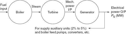
FIG. 2.1 Thermal generation system
2.3 SYSTEM VARIABLES
To analyze the power system network, there is a need of knowing the system variables. They are:
- Control variables.
- Disturbance variables.
- State variables.
2.3.1 Control variables (PG and QG)
The real and reactive-power generations are called control variables since they are used to control the state of the system.
2.3.2 Disturbance variables (PD and QD)
The real and reactive-power demands are called demand variables since they are beyond the system control and are hence considered as uncontrolled or disturbance variables.
2.3.3 State variables (V and δ)
The bus voltage magnitude V and its phase angle δ dispatch the state of the system. These are dependent variables that are being controlled by the control variables.
2.4 PROBLEM OF OPTIMUM DISPATCH—FORMULATION
Scheduling is the process of allocation of generation among different generating units. Economic scheduling is a cost-effective mode of allocation of generation among the different units in such a way that the overall cost of generation should be minimum. This can also be termed as an optimal dispatch.
Let the total load demand on the station = PD and the total number of generating units = n.
The optimization problem is to allocate the total load PD among these ‘n’ units in an optimal way to reduce the overall cost of generation.
Let PGi, PG2, PG3, …,PGn be the power generated by each individual unit to supply a load demand of PD.
To formulate this problem, it is necessary to know the ‘input–output characteristics of each unit’.
2.5 INPUT–OUTPUT CHARACTERISTICS
The idealized form of input–output characteristics of a steam unit is shown in Fig. 2.2. It establishes the relationship between the energy input to the turbine and the energy output from the electrical generator. The input to the turbine shown on the ordinate may be either in terms of the heat energy requirement, which is generally measured in Btu/hr or kCal/hr or in terms of the total cost of fuel per hour in Rs./hr. The output is normally the net electrical power output of that steam unit in kW or MW.
In practice, the curve may not be very smooth, and from practical data, such an idealized curve may be interpolated. The steam turbine-generating unit curve consists of minimum and maximum limits in operation, which depend upon the steam cycle used, thermal characteristics of material, the operating temperature, etc.
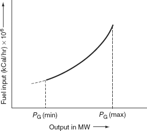
FIG. 2.2 Input–output characteristic of a steam unit
2.5.1 Units of turbine input
In terms of heat, the unit is 106 kcal/hr (or) Btu/hr or in terms of the amount of fuel, the unit is tons of fuel/hr, which becomes millions of kCal/hr.
2.6 COST CURVES
To convert the input–output curves into cost curves, the fuel input per hour is multiplied with the cost of the fuel (expressed in Rs./million kCal).
i.e., ![]()
|
= |
million kCal/hr × Rs./million kCal |
|
= |
Rs./hr |
2.7 INCREMENTAL FUEL COST CURVE
From the input–output curves, the incremental fuel cost (IFC) curve can be obtained.
The IFC is defined as the ratio of a small change in the input to the corresponding small change in the output.
Incremental fuel cost ![]()
where ∆ represents small changes.
As the ∆ quantities become progressively smaller, it is seen that the IFC is ![]() and is expressed in Rs./MWh. A typical plot of the IFC versus output power is shown in Fig. 2.3(a).
and is expressed in Rs./MWh. A typical plot of the IFC versus output power is shown in Fig. 2.3(a).
The incremental cost curve is obtained by considering the change in the cost of generation to the change in real-power generation at various points on the input–output curves, i.e., slope of the input–output curve as shown in Fig. 2.3(b).
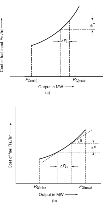
FIG. 2.3 (a) Incremental cost curve; (b) Incremental fuel cost characteristic in terms of the slope of the input–output curve
The IFC is now obtained as
(IC)i = slope of the fuel cost curve
i.e., tan β ![]()
The IFC (IC) of the ith thermal unit is defined, for a given power output, as the limit of the ratio of the increased cost of fuel input (Rs./hr) to the corresponding increase in power output (MW), as the increasing power output approaches zero.

where Ci is the cost of fuel of the ith unit and PG i is the power generation output of that ith unit.
Mathematically, the IFC curve expression can be obtained from the expression of the cost curve.
Cost-curve expression,
![]() (Second-degree polynomial)
(Second-degree polynomial)
The IFC,
![]() (linear approximation) for all i = 1, 2, 3, …, n
(linear approximation) for all i = 1, 2, 3, …, n
where ![]() is the ratio of incremental fuel energy input in Btu to the incremental energy output in kWh, which is called ‘the incremental heat rate’.
is the ratio of incremental fuel energy input in Btu to the incremental energy output in kWh, which is called ‘the incremental heat rate’.
The fuel cost is the major component and the remaining costs such as maintenance, salaries, etc. will be of very small percentage of fuel cost; hence, the IFC is very significant in the economic loading of a generating unit.
2.8 HEAT RATE CURVE
The heat rate characteristic obtained from the plot of the net heat rate in Btu/kWh or kCal/kWh versus power output in kW is shown in Fig. 2.4.
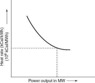
FIG. 2.4 Heat rate curve
The thermal unit is most efficient at a minimum heat rate, which corresponds to a particular generation PG. The curve indicates an increase in heat rate at low and high power limits.
Thermal efficiency of the unit is affected by the following factors: condition of steam, steam cycle used, re-heat stages, condenser pressure, etc.
2.9 INCREMENTAL EFFICIENCY
The reciprocal of the incremental fuel rate or heat rate, which is defined as the ratio of output energy to input energy, gives a measure of fuel efficiency for the input.
i.e., Incremental efficiency ![]()
2.10 NON-SMOOTH COST FUNCTIONS WITH MULTIVALVE EFFECT
For large steam turbine generators, the input–output characteristics are shown in Fig. 2.5(a).
Large steam turbine generators will have a number of steam admission valves that are opened in sequence to obtain an ever-increasing output of the unit. Figures 2.5(a) and (b) show input–output and incremental heat rate characteristics of a unit with four valves. As the unit loading increases, the input to the unit increases and thereby the incremental heat rate decreases between the opening points for any two valves. However, when a valve is first opened, the throttling losses increase rapidly and the incremental heat rate rises suddenly. This gives rise to the discontinuous type of characteristics in order to schedule the steam unit, although it is usually not done. These types of input–output characteristics are non-convex; hence, the optimization technique that requires convex characteristics may not be used with impunity.


FIG. 2.5 Characteristics of a steam generator unit with multivalve effect: (a) Input–output characteristic and (b) incremental heat rate characteristic
2.11 NON-SMOOTH COST FUNCTIONS WITH MULTIPLE FUELS
Generally, a piece-wise quadratic function is used to represent the input–output curve of a generator with multiple fuels. Figure 2.6 represents the incremental heat rate characteristics of a generator with multiple fuels.
2.12 CHARACTERISTICS OF A HYDRO-POWER UNIT
A simple hydro-power plant is shown in Fig. 2.7(a).
The input–output characteristics of a hydro-power unit as shown in Fig. 2.7(b) can be obtained in the same way as for the steam units assuming the water head to be constant. The ordinates are water input or discharge (m3/s) versus output power (kW or MW).
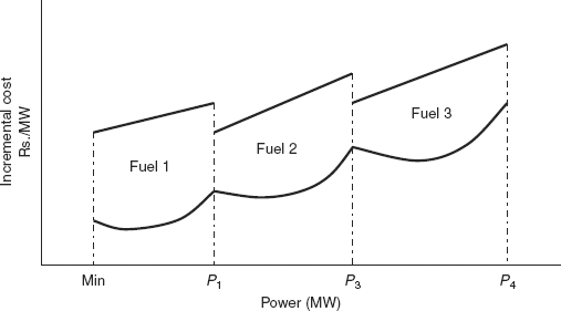
FIG. 2.6 Incremental heat-rate characteristics of a steam generator with multiple fuels

FIG. 2.7 (a) A typical system of a hydro-power plant; (b) Input–output characteristics of a hydro-unit; (c) Effect of water head on water discharge; (d) Incremental water rate characteristic of a hydro-unit; (e) Incremental cost characteristic of a hydro-unit
From Fig. 2.7(b), it is observed that there is a linear water requirement upto the rated load and after that greater discharge is needed to meet the increased load demand such that the efficiency of the unit decreases.
2.12.1 Effect of the water head on discharge of water for a hydro-unit
Figure 2.7(c) shows the effect of the water head on water discharge. It is observed that when the head of the water falls, the input–output characteristic of a hydro-power plant moves vertically upwards, such that a higher discharge of water is needed for the same power generation. The reverse will happen when the head rises.
2.12.2 incremental water rate characteristics of hydro-units
A typical incremental water rate characteristic is shown in Fig. 2.7(d). It can be obtained from the input–output characteristic of a hydro-unit as shown in Fig. 2.7(b).
From Fig. 2.7(d), it is seen that the curve is a straight horizontal line upto the rated load indicating a constant slope and after that it rises rapidly. When the load increases more than the rated, more units will be put into operation (service).
2.12.3 Incremental cost characteristic of a hydro-unit
Actually, the input of a hydro-plant is not dependent on the cost. But the input water flow costs are due to the capacity of storage, requirement of water for the agricultural purpose, and running of the plant during off season (dry season). The artificial storage requirement (i.e., cost of construction of dams, canals, conduits, gates, penstocks, etc.) imposes a cost on the water input to the turbine as well as the cost of control on the water output from the turbine due to agricultural need.
The incremental cost characteristic can be obtained from the incremental water rate characteristic by multiplying it with cost of water in Rs./m3.
Incremental cost |
= |
(Incremental water rate) × cost of water in Rs./m3 |
|
= |
m3/MWh × Rs./m3 |
|
= |
Rs./MWh |
The incremental cost characteristic (or) incremental production cost characteristic is shown in Fig. 2.7(e).
The analytical expression of an incremental cost characteristic is
(IC)H |
= |
C1, (0 ≤ PGH ≤ PGH1) |
|
= |
m PGH + C1, ( PGH1 ≤ PGH ≤ PGH2) |
where PGH is the power generation of a hydro-unit and m is the slope of characteristic between PGH1 and PGH2.
2.12.4 Constraints of hydro-power plants
The following constraints are generally used in hydro-power plants.
(i) Water storage constraints
Let γ j be the storage volume at the end of interval j, γmin ≤ γ j ≤ γmax.
(ii) Water spillage constraints
Even though there may be circumstances where allowing water spillage (SPj) > 0 for some interval j, prohibition of spillage is assumed so that all SPj = 0 might reduce the cost of operation of a thermal plant.
(iii) Water discharge flow constraints
The discharge flow may be constrained both in rate and in total as
2.13 INCREMENTAL PRODUCTION COSTS
The incremental production cost of a given unit is made up of the IFC plus the incremental cost of items such as labor, supplies, maintenance, and water.
It is necessary for a rigorous analysis to be able to express the costs of these production items as a function of output. However, no methods are presently available for expressing the cost of labor, supplies, or maintenance accurately as a function of output.
Arbitrary methods of determining the incremental costs of labor, supplies, and maintenance are used, the commonest of which is to assume these costs to be a fixed percentage of the IFCs.
In many systems, for purposes of scheduling generation, the incremental production cost is assumed to be equal to the IFC.
2.14 CLASSICAL METHODS FOR ECONOMIC OPERATION OF SYSTEM PLANTS
Previously, the following thumb rules were adopted for scheduling the generation among various units of generators in a power station:
- Base loading to capacity: The turbo-generators were successively loaded to their rated capacities in the order of their efficiencies.
- Base loading to most efficient load: The turbo-generator units were successively loaded to their most efficient loads in the increasing order of their heat rates.
- Proportional loading to capacity: The turbo-generator sets were loaded in proportion to their rated capacities without consideration to their performance characteristics.
If the incremental generation costs are substantially constant over the range of operation, then without considering reserve and transmission line limitations, the most economic way of scheduling generation is to load each unit in the system to its rated capacity in the order of the highest incremental efficiency. This method, known as the merit order approach to economic load dispatching, requires the preparation of the order of merit tables based upon the incremental efficiencies, which should be updated regularly to reflect the changes in fuel costs, plant cycle efficiency, plant availability, etc. Active power scheduling then involves looking into the tables without the need for any calculations.
2.15 OPTIMIZATION PROBLEM—MATHEMATICAL FORMULATION (NEGLECTING THE TRANSMISSION LOSSES)
An optimization problem consists of:
- Objective function.
- Constraint equations.
2.15.1 Objective function
The objective function is to minimize the overall cost of production of power generation.
Cost in thermal and nuclear stations is nothing but the cost of fuel. Let n be the number of units in the system and Ci the cost of power generation of unit ‘i ’:
∴ Total cost C = C1 + C2 + C3 + … + Cn
i.e., ![]()
The cost of generation of each unit in thermal power plants is mainly a fuel cost. The generation cost depends on the amount of real power generated, since the real-power generation is increased by increasing the fuel input.
The generation of reactive power has negligible influence on the cost of generation, since it is controlled by the field current.
Therefore, the generation cost of the i th unit is a function of real-power generation of that unit and hence the total cost is expressed as
i.e., C = C1 (PG1) + C2 (PG2) + C3 (PG3) + … + Cn (PGn)
This objective function consists of the summation of the terms in which each term is a function of separate independent variables. This type of objective function is called a separable objective function.
The optimization problem is to allocate the total load demand (PD) among the various generating units, such that the cost of generation is minimized and satisfies the following constraints.
2.15.2 Constraint equations
The economic power system operation needs to satisfy the following types of constraints.
(1) Equality constraints
The sum of real-power generation of all the various units must always be equal to the total real-power demand on the system.
i.e., ![]()
or
where ![]() total real-power generation and PD is the total real-power demand. Equation (2.2) is known as the real-power balance equation when losses are neglected.
total real-power generation and PD is the total real-power demand. Equation (2.2) is known as the real-power balance equation when losses are neglected.
(2) Inequality constraints
These constraints are considered in an economic power system operation due to the physical and operational limitations of the units and components.
The inequality constraints are classified as:
(a) According to the nature
According to nature, the inequality constraints are classified further into the following constraints:
- Hard-type constraints: These constraints are definite and specific in nature. No flexibility will take place in violating these types of constraints.
e.g.,: The range of tapping of an on-load tap-changing transformer.
- Soft-type constraints: These constraints have some flexibility with them in violating.
e.g.,: Magnitudes of node voltages and the phase angle between them.
Some penalties are introduced for the violations of these types of constraints.
(b) According to power system parameters
According to power system parameters, inequality constraints are classified further into the following categories.
- Output power constraints: Each generating unit should not operate above its rating or below some minimum generation. This minimum value of real-power generation is determined from the technical feasibility.
PGi(min) ≤ PGi ≤ PGi(max) (2.3a)
Similarly, the limits may also have to be considered over the range of reactive-power capabilities of the generator unit requiring that:
QGi(min) ≤ QGi ≤ QGi(max) for i = 1, 2, 3, …, n (2.3b)and the constraint P2Gi + Q2Gi ≤ (S irated)2 must be satisfied, where Si is the rating of the generating unit for limiting the overheating of stator.
- Voltage magnitude and phase-angle constraints: For maintaining better voltage profile and limiting overloadings, it is essential that the bus voltage magnitudes and phase angles at various buses should vary within the limits. These can be illustrated by imposing the inequality constraints on bus voltage magnitudes and their phase angles.
Vi (min) ≤ Vi ≤ Vi (max) for i = 1, 2, …, n
δij (min) ≤ δij ≤ δij (max) for i = 1, 2, …, n
where j = 1, 2, …, m, j ≠ i, n is the number of units, and m the number of loads connected to each unit.
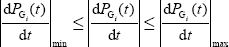
- Dynamic constraints: These constants may consider when fast changes in generation are required for picking up the shedding down or increasing of load demand. These constraints are of the form:
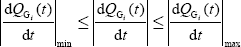
In addition, in terms of reactive-power generation,
- Spare capacity constraints: These constraints are required to meet the following criteria:
- Errors in load prediction.
- The unexpected and fast changes in load demand.
- Unplanned loss of scheduled generation, i.e., the forced outages of one or more units on the system.
The total power generation at any time must be more than the total load demand and system losses by an amount not less than a specified minimum spare capacity (PSP)
i.e., PG ≥ (PD + PL) + PSP
where PG is the total power generation, PD + PL is the total load demand and system losses, and PSP is the specified minimum spare power.
- Branch transfer capacity constraints: Thermal considerations may require that the transmission lines be subjected to branch transfer capacity constraints:
Si (min) ≤ Sbi ≤ Si (max) for i = 1, 2, …, nb
where nb is the number of branches and Sbi the i th branch transfer capacity in MVA.
- Transformer tap position/settings constraints: The tap positions (or) settings of a transformer (T) must lie within the available range:
T(min) ≤ T ≤ T(max)
For an autotransformer, the tap setting constraints are:
0 ≤ T ≤ 1
where the minimum tap setting is zero and the maximum tap setting is 1.
For a 2-winding transformer, tap setting constraints are 0 ≤ T ≤ K, where K is the transformation (turns) ratio.
For a phase-shifting transformer, the constraints are of the type:
θi (min) ≤ θi ≤ θi (max)
where θi is the phase shift obtained from the i th transformer.
- Transmission line constraints: The active and reactive power flowing through the transmission line is limited by the thermal capability of the circuit.
TCi ≤ TCi (max)
where TCi (max) is the maximum loading capacity of the i th line.
- Security constraints: Power system security and power flows between certain important buses are also considered for the solution of an optimization problem.
If the system is operating satisfactorily, there is an outage that may be scheduled or forced, but some of the constraints are naturally violated. It may be mentioned that consideration of each and every possible branch for an outage will not be a feasible proportion. When a large system is under study, the network security is maintained such that computation is to be made with the outage of one branch at one time and then the computation of a group of branches or units at another time.
So, the optimization problem was stated earlier as minimizing the cost function (C) given by Equation (2.1), which is subjected to the equality and inequality constraint (Equations (2.2) and (2.3)).
2.16 MATHEMATICAL DETERMINATION OF OPTIMAL ALLOCATION OF TOTAL LOAD AMONG DIFFERENT UNITS
Consider a power station having ‘n’ number of units. Let us assume that each unit does not violate the inequality constraints and let the transmission losses be neglected.
The cost of production of electrical energy
where Ci is the cost function of the i th unit.
This cost is to be minimized subject to the equality constraint given by
where PGi is the real-power generation of the ith unit.
This is a constrained optimization problem.
To get the solution for the optimization problem, we will define an objective function by augmenting Equation (2.4) with an equality constraint (Equation (2.5)) through the Lagrangian multiplier (λ) as
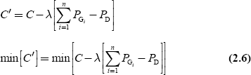
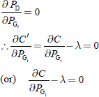
The condition for optimality of such an augmented objective function is
![]()
From Equation (2.6),
Since PD is a constant and is an uncontrolled variable,

Since the expression of C is in a variable separable form, i.e., the overall cost is the summation of cost of each generating unit, which is a function of real-power generation of that unit only:

In Equation (2.8), each of these derivatives represents the individual incremental cost of every unit. Hence, the condition for the optimal allocation of the total load among the various units, when neglecting the transmission losses, is that the incremental costs of the individual units are equal. It a called a co-ordination equation.
Assume that one unit is operating at a higher incremental cost than the other units. If the output power of that unit is reduced and transferred to units with lower incremental operating costs, then the total operating cost decreases. That is, reducing the output of the unit with the higher incremental cost results in a more decrease in cost than the increase in cost of adding the same output reduction to units with lower incremental costs. Therefore, all units must run with same incremental operating costs.
After getting the optimal solution, in the case that the generation of any one unit is below its minimum capacity or above its maximum capacity, then its generation becomes the corresponding limit. For example, if the generation of any unit violates the minimum limit, then the generation of that unit is set at its minimum specified limit and vice versa. Then, the remaining demand is allocated among the remaining units as for the above criteria.
In the solution of an optimization problem without considering the transmission losses, we make use of equal incremental costs, i.e., the machines are so loaded that the incremental cost of production of each machine is the same.
It can be seen that this method does not sense the location of changes in the loads. As long as the total load is fixed, irrespective of the location of loads, the solution will always be the same and, in fact, for this reason the solution may be feasible in the sense that the load voltages may not be within specified limits. The reactive-power generation required may also not be within limits.
2.17 COMPUTATIONAL METHODS
Different types of computational methods for solving the above optimization problem are as follows:
- Analytical method.
- Graphical method.
- Using a digital computer.
The method to be adopted depends on the following:
- The mathematical equation representing the IFC of each unit, which can be determined from the cost of generation of that unit.
The cost of the ith unit is given by

∴ The IFC of the ith unit
(IC)i = aiPGi + bi (Linear model) (2.10)
where ai is the slope of the IFC curve and bi the intercept of the IFC curve.
- Number of units (n).
- Need to represent the discontinuities (if any due to steam valve opening) in the IFC curve.
2.17.1 Analytical method
When the number of units are small (either 2 or 3), incremental cost curves are approximated as a linear or quadratic variation and no discontinuities are present in the incremental cost curves.
We know that the IFC of the i th unit
![]()
For an optimal solution, the IFC of all the units must be the same (neglecting the transmission losses):
The analytical method consists of the following steps:
- Choose a particular value of λ.
i.e., λ = aiPG1 + bi
- Compute

- Find total real-power generation
 for all i = 1, 2, …, n.
 - Repeat the procedure from step (ii) for different values of λ.
- Plot a graph between total power generation and λ.
- For a given power demand (PD), estimate the value of λ from Fig. 2.8.
That value of λ will be the optimal solution for optimization problem.
2.17.2 Graphical method
For obtaining the solution in this method, the following procedure is required:
- (i) Consider the incremental cost curves of all units:
i.e., (IC)i = ai PGi + bi for all i = 1, 2, …, n
and the total load demand PD is given.

FIG. 2.8 Estimation of optimum value of λ—analytical method

FIG. 2.9 Graphical method
- For each unit, draw a graph between PG and (IC) as shown in Fig. 2.9.
- Choose a particular value of λ and ∆λ.
- Determine the corresponding real-power generations of all units:
i.e., PG1, PG2, …, PGn
- Compute the total real-power generation

- Check the real-power balance of Equation (2) as follows:
- If
 , then the λ chosen will be the optimal solution and incremental costs of all units become equal.
 - If
 , increase λ by ∆λ and repeat the procedure from step (iv).
 - If
 , decrease λ by ∆λ and repeat the procedure from step (iv).
- If
- This process is repeated until
 is within a specified tolerance (ε), say 1 MW.
2.17.3 Solution by using a digital computer
For more number of units, the λ-iterative method is more accurate and incremental cost curves of all units are to be stored in memory.
information about the IFC curves is given for all units:
i.e., λ = (IC)i = aiPGi + bi
or ![]() (when losses are neglected)
(when losses are neglected)
and so on.
for i = 1, 2, …, n
The number of terms included depends on the degree of accuracy required and coefficients αi, βi, and γi are to be taken as input.
Algorithm for λ –Iterative Method
- Guess the initial value of λo with the use of cost-curve equations.
- Calculate PoG1, according to Equation (2.14), i.e., PoG1 = αi + βi (λo)i + γi(λo)2i + …
- Calculate

- Check whether
 :
:

- If
 set a new value for λ, i.e., λ′ = λo + ∆λ and repeat from step (ii) till the tolerance value is satisfied.
 - If
 set a new value for λ, i.e., λ′ = λo – ∆λ and repeat from step (ii) till the tolerance value is satisfied.
 - Stop.
Example 2.1: The fuel cost functions in Rs./hr for three thermal plants are given by
C1 = 400 + 8.4P1 + 0.006P12
C2 = 600 + 8.93P2 + 0.0042P22
C3 = 650 + 6.78P3 + 0.004P32
where P1, P2, and P3 are in MW. Neglecting line losses and generator limits, determine the optimal scheduling of generation of each loading using the iterative method.
- PD = 550 MW.
- PD = 820 MW.
- PD = 1,500 MW.
Solution:
For (i) PD = 550 MW:
%MATLAB PROGRAM FOR ECONOMIC LOAD DISPATCH NEGLECTING LOSSES AND
GENERATOR LIMITS(dispatch1.m)
clc;
clear;
|
%undo |
d |
b |
a |
Cost data = |
[1 |
400 |
8.4 |
0.006; |
|
2 |
600 |
8.93 |
0.0042; |
|
3 |
650 |
6.78 |
0.004]; |
Ng = length(cost data(:,1));
for i = 1:ng
uno(i) = cost data(i,1);
a(i) = cost data(i,2);
b(i) = cost data(i,3);
d(i) = cost data(i,4);
end
lambda = 9.0;
pd = 550;
delp = 0.1;
dellambda = 0;
iter = 0;
while(abs(delp)> = 0.001)
iter = iter+1;
lambda = lambda + dellambda;
sum = 0;
totgam = 0;
for i = 1:ng
p(i) = (lambda-b(i))/(2*d(i));
sum = sum + p(i);
totgam = totgam + 0.5*(1/d(i));
ifc(i) = lambda;
end
delp = pd–sum;
dellambda = delp/totgam;
end
totgencost = 0;
for i = 1:ng
totgencost = totgencost + (a(i)+ b(i)*p(i)+ d(i)*p(i)*p(i));
end
disp(‘OUTPUT OF MATLAB PROGRAM dispatch1.m’);
lambda
disp(‘GENERATING UNIT OPTIMAL GENERATION(MW)’);
[uno; p]’
disp(‘INCREMENTAL FUEL COST’);
ifc(1)
OUTPUT OF MATLAB PROGRAM dispatch1.m
lambda = 9.6542
GENERATING UNIT |
OPTIMAL GENERATION(MW) |
1 |
104.5152 |
2 |
86.2121 |
3 |
359.2727 |
INCREMENTAL FUEL COST (Rs./MWhr) = 9.6542
TOTAL GENERATION COST(Rs./hr) = 6346.70
For (ii) PD = 820 MW:
OUTPUT OF MATLAB PROGRAM dispatch1.m
lambda = 10.4789
GENERATING UNIT |
OPTIMAL GENERATION(MW) |
1.0000 |
173.2424 |
2.0000 |
184.3939 |
3.0000 |
462.3636 |
INCREMENTAL FUEL COST(Rs./MWhr) = 10.4789
TOTAL GENERATION COST(Rs./hr) = 9064.70
For (iii) PD = 1,500 MW:
OUTPUT OF MATLAB PROGRAM dispatch1.m
lambda = 12.5560
GENERATING UNIT |
OPTIMAL GENERATION(MW) |
1.0000 |
346.3333 |
2.0000 |
431.6667 |
3.0000 |
722.0000 |
INCREMENTAL FUEL COST(Rs./MWhr) = 12.5560
TOTAL GENERATION COST(Rs./hr) = 16897.00
2.18 ECONOMIC DISPATCH NEGLECTING LOSSES AND INCLUDING GENERATOR LIMITS
The output power of any generator should neither exceed its rating nor should it be below that necessary for the stable operation of a boiler. Thus, the generations are restricted to lie within given minimum and maximum limits. The problem is to find the active power generation of each plant such that the objective function (i.e., total production cost) is minimum, subject to the equality constraint, and the inequality constraints are
respectively.
The solution algorithm for this case is the same as discussed in Section 2.17.3 with minor modifications. If any generating unit violates the above inequality constraints, set its generation at its respective limit as given below. In addition, the balance of the load is then shared between the remaining units on the basis of equal incremental cost.
The necessary conditions for optimal dispatch when losses are neglected:
![]() for PGi(min) ≤ PGi ≤ PGi(max)
for PGi(min) ≤ PGi ≤ PGi(max)
![]() for PGi = ≤ PGi(max)
for PGi = ≤ PGi(max)
![]() for ≤ PGi = ≤ PGi(min)
for ≤ PGi = ≤ PGi(min)
Example 2.2: The fuel cost functions in Rs./hr. for three thermal plants are given by
C1 = 400 + 8.4P12, |
100 ≤ P1 ≤ 600 |
C2 = 600 + 8.93P22, |
60 ≤ P2 ≤ 300 |
C3 = 650 + 6.78P32, |
300 ≤ P3 ≤ 650 |
where P1, P2, and P3 are in MW. Neglecting line losses and including generator limits, determine the optimal scheduling of generation of each loading using the iterative method.
- PD = 550 MW.
- PD = 820 MW.
- PD = 1,500 MW.
Solution:
For (i) P D = 550 MW:
%MATLAB PROGRAM FOR ECONOMIC LOAD DISPATCH NEGLECTING LOSSES AND
INCLUDING
%GENERATOR LIMITS(dispatch2.m)
clc;
clear;

ng = length(cost data(:,1));
for i = 1:ng
uno(i)= cost data(i,1);
a(i)= cost data(i,2);
b(i)= cost data(i,3);
d(i)= cost data(i,4);
pmin (i)= cost data(i,5);
pmax (i)= cost data(i,6);
end
lambda = 9.0;
pd = 550;
delp = 0.1;
dellambda = 0;
for i = 1:ng
pv(i) = 0;
pvfin(i) = 0;
end
while(abs(delp)>= 0.0001)
lambda = lambda + dellambda;
sum = 0;
totgam = 0;
for i = 1:ng
p(i) = (lambda–b(i))/(2*d(i));
sum = sum + p(i);
totgam = totgam+0.5*(1/d(i));
end
delp = pd – sum;
dellambda = delp/totgam;
ifc = lambda;
end
limvio = 0;
for i = 1:ng
if(p(i) < pmin(i)|p(i) > pmax(i))
limvio = 1;
break;
end
end
if limvio = = 0
disp(‘GENERATION IS WITHIN THE LIMITS’);
end
if (1imvio = = 1)
sum = 0;
totgam = 0;
delp = 0.1;
loprep = 1;
while(abs(delp) >= 0.01 & loprep = 1)
disp(‘GENERATION IS NOT WITHIN THE LIMITS’);
disp(‘VIOLATED GENERATOR NUMBER’);
i
if p(i) < pmin(i)
disp(‘GENERATION OF VIOLATED UNIT(MW)’);
p(i)
disp(‘CORRESPONDING VOILATED LIMIT IS pmin’);
elseif p(i) > pmax(i)
disp(‘GENERATION OF VIOLATED UNIT(MW)’);
p(i)
disp(‘CORRESPONDING VIOLATED LIMIT IS pmax’);
end
sum = 0;
totgam = 0;
for i = 1:ng
pv(i) = 0;
end
for i = 1:ng
if (p(i) < pmin(i)|p(i) > pmax(i))
if p(i) < pmin(i)
p(i) = pmin(i);
else
p(i) = pmax(i);
end
pv(i) = 1;
pvfin(i) = 1;
break;
end
end
for i = 1:ng
sum = sum + p(i);
if (pvfin(i) ~= 1)
totgam = totgam + 0.5*(1/d(i));
end
end
delp = pd – sum;
dellambda = delp/totgam;
lambda = lambda+dellambda;
ifc = lambda;
for i = 1:ng
if pvfi n(i) ~ = 1
p(i) = (lambda–b(i))/(2*d(i));
end
sum = sum + p(i);
end
delp = pd–sum;
loprep = 0;
for i = 1:ng
if p(i) < pmin(i)|p(i) > pmax(i)
loprep = 1;
break;
end
end
end
end
totgencost = 0;
for i = 1:ng
totgencost = totgencost+(a(i)+b(i)*p(i)+d(i)*p(i)*p(i));
end
disp(‘FINAL OUTPUT OF MATLAB PROGRAM dispatch2.m’);
lambda
disp(‘GENERATING UNIT OPTIMAL GENERATION(MW)’);
[uno; p]’
disp(‘INCREMENTAL FUEL COST(Rs./MWhr)’);
ifc
disp(‘TOTAL GENERATION COST(Rs./hr.)’);
totgencost
Results for (i) Pd = 550 MW:
GENERATION IS WITHIN THE LIMITS
FINAL OUTPUT OF MATLAB PROGRAM dispatch2.m
lambda = 9.6542
GENERATING UNIT |
OPTIMAL GENERATION(MW) |
1.0000 |
104.5152 |
2.0000 |
86.2121 |
3.0000 |
359.2727 |
INCREMENTAL FUEL COST (Rs./MWhr) = 9.6542
TOTAL GENERATION COST(Rs./hr) = 6346.70
Results for (ii) Pd = 820 MW:
GENERATION IS WITHIN THE LIMITS
FINAL OUTPUT OF MATLAB PROGRAM dispatch2.m
lambda = 10.4789
GENERATING UNIT |
OPTIMAL GENERATION(MW) |
1.000 |
173.2424 |
2.0000 |
184.3939 |
3.0000 |
462.3636 |
INCREMENTAL FUEL COST (Rs./MWhr)=10.4789
TOTAL GENERATION COST (Rs./hr) = 9064.70
Results for (iii) Pd = 1,500 MW:
GENERATION IS NOT WITHIN THE LIMITS
VIOLATED GENERATOR NUMBER = 2
GENERATION OF VIOLATED UNIT (MW) = 431.6667
CORRESPONDING VIOLATED LIMIT IS pmax
GENERATION IS NOT WITHIN THE LIMITS
VIOLATED GENERATOR NUMBER = 3
GENERATION OF VIOLATED UNIT (MW) = 801
CORRESPONDING VIOLATED LIMIT IS pmax
FINAL OUTPUT OF MATLAB PROGRAM dispatch2.m
lambda = 15
GENERATING UNIT |
OPTIMAL GENERATION(MW) |
1 |
550 |
2 |
300 |
3 |
650 |
INCREMENTAL FUEL COST (Rs./MWhr) = 15
TOTAL GENERATION COST (Rs./hr) = 17239
2.19 FLOWCHART FOR OBTAINING OPTIMAL SCHEDULING OF GENERATING UNITS BY NEGLECTING THE TRANSMISSION LOSSES
The optimal scheduling of generating units is represented by the flowchart as shown in Fig. 2.10.
2.20 ECONOMICAL LOAD DISPATCH—IN OTHER UNITS
The economical load dispatch problem has been solved for a power system area consisting of fossil fuel units. For an area consisting of a mix of different types of units, i.e.— fossil fuel units, nuclear units, pumped storage hydro-units, hydro-units, etc.—solving the economical load dispatch problem will become different.
2.20.1 Nuclear units
For these units, the fixed cost is high and operating costs are low. As such, nuclear units are generally base load plants at their rated outputs, i.e., the reference power setting of turbine governors for nuclear units is held constant at the rated output. Therefore, these units do not participate in economical load dispatch.
2.20.2 Pumped storage hydro-units
These units are operated as synchronous motors to pump water during off-peak hours. During peak load hours, the water is released and the units are operated as synchronous generators to supply power. The economic operation of the area is done by pumping during off-peak hours when the area incremental cost (λ) is low, and by generating during peak load hours when λ is high. Some techniques are available for incorporating pumped storage hydro-units into the economic dispatch of fossil units.
2.20.3 Hydro-plants
For an area consisting of hydro-plants located along a river, the objective of the economic dispatch problem becomes maximizing the power generation over the yearly water cycle rather than minimizing the total operating costs. For these types of plants, reservoirs are provided to store the water during rainy seasons. There are some constraints on the level of water such as flow of river, irrigation, etc. Optimal strategies are available for co-ordinating the outputs of such plants along a river. There are also some economic dispatch strategies available for the mix of fossil fuel and hydro-systems.

2.20.4 Including reactive-power flows
In this case, both active and reactive powers are selected to minimize the operating costs. In particular, reactive-power injections from generators, switched capacitor banks, and static VAr systems along with transformer settings can be selected to minimize the transmission losses.
Example 2.3: A system consists of two units to meet the daily load cycle as shown in Fig. 2.11.
The cost curves of the two units are:
C1 = 0.15 P2G1 + 60 PG1 + 135 Rs./hr
C1 = 0.25 P2G2 + 40 PG2 + 110 Rs./hr
The maximum and minimum loads on a unit are to be 220 and 30 MW, respectively.
Find out:
- The economical distribution of a load during the light-load period of 7 hr and during the heavy-load periods of 17 hr. In addition, find the operation cost for this 24-hr period operation of two units.
- The operation cost when removing one of the units from service during 7 hr of light-load period.
Assume that a cost of Rs. 525 is incurred in taking a unit off the line and returning it to service after 7 hr. - Comment on the results.
Solution:
(i) When both units are operating throughout a 24-hr period,
Total time = 24 hr
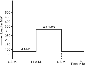
FIG. 2.11 Daily load cycle
Total load = 84 MW for 7 hr + 400 MW for 17 hr
(from 4 A.M. to 11 A.M.) (from 11 A.M. to 4 A.M.)
For a heavy load of 400 MW:
Heavy-load period, th =17 hr
load, PDh = 400 MW
We have to find the optimal scheduling of two units with this load.
We have the cost curves of two units:
For Unit 1:
C1 = 0.15 P2G1 + 60 PG1 + 135 Rs./hr
Incremental fuel cost, ![]()
= 0.3 PG1 + 60 Rs./MWh
For Unit 2:
C2 = 0.25 P2G2 + 40 PG2 + 110 Rs./hr
![]() 0.25 × 2 PG2 + 40
0.25 × 2 PG2 + 40
= 0.5 PG2 + 40 Rs./MWh
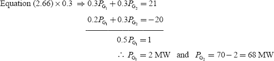
For the optimal distribution of a load,
![]()
0.3PG1 + 60 = 0.5 PG2 + 40
0.3PG1 − 0.5 PG2 = − 20 (2.15)
PG1 + PG2 = 400 (given) (2.16)
From Equations (2.15) and (2.16), we have

Substituting the PG1 value in Equation (2.16), we get
Here, PG1 = 225 MW and PG1 > PGmax; hence, set PG1 at its maximum generation limit
i.e., PG1 = 220 MW
∴ PG2 = 400 - 220 = 180 MW
The operation cost for a heavy-load period (i.e., from 11 A.M. to 4 A.M.) with this optimal distribution is
C |
= |
(C1 + C2) × th |
|
= |
[(0.15 × 2202 + 60 × 220 + 135) + (0.25 × 1802 + 40 × 180 + 110)] × 17 |
|
= |
Rs. 6,12,085 |
For a light load of 84 MW:
Period, tl = 7 hr
load, PD = 84 MW
For optimal load sharing,
i.e., 0.3 PG1 + 60 = 0.5 PG2 + 40
0.3 PG1 − 0.5 PG2 = − 20 (2.17)
PG1 + PG2 = 84 (2.18)
By solving Equations (2.17) and (2.18), we get
PG1 = 27.5 MW; PG2 = 56.5 MW
Here, PG1 = 27.5 MW < PGmin = 30 MW
Therefore, the load shared by Unit-1 is set to PG1 = 30 MW and PG2 = 84 - 30 = 54 MW.
The operation cost for a light-load period (i.e., from 4 A.M. to 11 A.M.) with this optimal distribution:
= [(0.15) × (30)2 + 60 ×30 + 135) + (0.25 × 542 + 40 × 54 + 110)] × 7
= Rs. 35,483
Hence, the total fuel cost when both the units are operating throughout the 24-hr period
= Rs. (6,12,085 + 35,483)
= Rs. 6,47,568
(ii)If only one of the units is run during the light-load period,
i.e., Period, tl = 7 hr
load, PD = 84 MW
When Unit-1 is to be run,
Cost of operation |
= |
C1 × t1 |
|
= |
[0.15 × 842 + 60 × 84 + 135] × 7 |
|
= |
Rs 43,633.80 |
When Unit-2 is to be run,
Cost of operation |
= |
C2 × t1 |
|
= |
[0.15 × 842 + 40 × 84 + 110] × 7 |
|
= |
Rs 36,638 |
From the above, it is verified that it is economical to run Unit-2 during a light-load period and to put off Unit-1 from service.
The operating cost with only Unit-2 in operation = Rs. 36,638
The operating cost for the operation of both units in a heavy-load period and Unit-2 only in a light-load period = Rs. (6,47,568 + 36,638) = Rs. 6,48,723
In addition, given that a cost of Rs. 525 is incurred in taking a unit off the line and returning it to service after 7 hr,
Total operating cost = operating cost + start-up cost = Rs. (6,48,723 + 525) = Rs. 6,49,248.
(iii) Total operating cost for (i) = Rs. 6,47,568
Total operating cost for (ii) = Rs. 6,49,248
It is concluded that the total operating cost when both units running throughout 24-hr periods is less than the operating cost when one of the units is put off from the line and returned to the service after a light-load period. Hence, it is economical to run both units throughout 24 hr.
Example 2.4: A constant load of 400 MW is supplied by two 210-MW generators 1 and 2, for which the fuel cost characteristics are given as below:
C1 = 0.05 P2G1 + 20 PG1 + 30.0 Rs./hr
C2 = 0.06 P2G2 + 15 PG1 + 40.0 Rs./hr
The real-power generations of units PG1 and PG2 are in MW. Determine: (i) the most economical load sharing between the generators. (ii) The saving in Rs./day thereby obtained compared to the equal load sharing between two generators.
Solution:
The IFCs are
![]() = 0.10 PG1 + 20.0
= 0.10 PG1 + 20.0
![]() = 0.12 PG2 + 15.0
= 0.12 PG2 + 15.0
(i) For optimal sharing of load, the condition is
![]()
|
0.10 PG1 + 20.0 = 0.12 PG1 + 15.0 |
|
or |
0.10 PG1 − 0.12 PG1 = 15.0 − 20.0 |
|
or |
0.10 PG1 − 0.12 PG1 = − 5.0 |
(12.19) |
|
Given: PG1 + PG2 = 400 |
(12.20) |
Solving Equations (2.19) and (2.20), we have
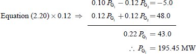
Substituting PG1 = 195.45 MW in Equation (2.20), we get
PG2 = 400 – 195.45 = 204.55 MW
The load of 400 MW is economically shared by the two generators with PG1 = 195.45 MW and PG2 = 204.55 MW.
(ii) When the load is shared between the generators equally, then
PG1 = 200 MW and PG2 = 200 MW
With this equal sharing of load, the PG1 value is increased from 195.45 with economical sharing to 200 MW.
∴ Increase in operation cost of generator 1

The PG2 value is decreased from 204.55 to 200 MW.
∴ Decrease in operation cost of Generator 2
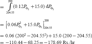
∴ Saving in cost = 180.96 – 178.69 = 2.27 Rs./hr
The saving in cost per day = 2.27 × 24
Example 2.5: Consider the following three IC curves:
PG1 |
= |
− 100 + 50(IC1) + 2(IC1)2 |
PG2 |
= |
− 150 + 60(IC2) − 2(IC2)2 |
PG3 |
= |
− 80 + 40(IC3) − 1.8(IC3)2 |
where IC’s are in Rs./MWh and PG’s are in MW.
The total load at a certain hour of the day is 400 MW. Neglect transmission losses and develop a computer program for optimum generation scheduling within the accuracy of ± 0.05 MW.
Note: All PG’s must be real and positive.
α1 = −100, |
β1 = 50, |
γ1 = 2 (∵ Assume d1, d2, d3 are neglected) |
α2 = −150, |
β2 = 60, |
γ2 = −2.5 |
α3 = −80, |
β3 = 40, |
γ3 = −1.8 |
αi = ![]()
∴ a1 = 0.02; a2 = 0.0166; a3 = 0.025
b1 = 2; b2 = 2.49; b3 = 2
![]()
![]()
![]()
For optimal load distribution among the various units,

0.02 PG1 + 2 = 0.0166 PG2 + 2.49 |
|
⇒ 0.02 PG1 − 0.0166 PG2 = 0.49 |
(2.21) |
![]()
0.0166PG2 + 2.49 = 0.025 PG3 + 2 |
|
0.0166 PG2 − 0.025 PG3 = − 0.49 |
(2.22) |
![]()
0.02 PG1 + 2 = 0.025 PG3 + 2
0.02 PG1 − 0.025 PG3 = 0 (2.23)
Given: PG1 + PG2 + PG3 = 400 (2.24)
or PG2 + PG3 = 400 − PG1 (2.25)
Solving Equations (2.22) and (2.25), we have

0.0166 PG1 + 0.0416 PG3 = 7.13 (2.26)
Solving Equations (2.23) and (2.26), we get
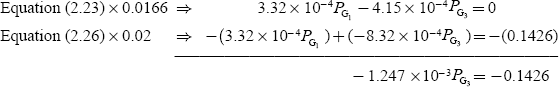
![]()
Substituting PG3 |
= |
14.35 MW in (2.26), we get |
PG1 |
= |
142.9375 MW |
Substituting PG1 |
= |
142.9375 MW and PG3 = 114.35 MW in (2.25), we get |
PG2 |
= |
142. 93175 MW |
Therefore, for optimal generation, the three units must share a total load of 400 MW as follows:
Cost of generation of 142.9375 MW by Unit-1
(C1) = ![]() (142.9375)2 + 2 (142.9375)
(142.9375)2 + 2 (142.9375)
C1 = 490.186 Rs. / MWh
Similarly,

and C3 = ![]() × 0.025 × (114.35)2 + (2 × 114.35)
× 0.025 × (114.35)2 + (2 × 114.35)
= 392.149 Rs. / MWh
Total cost of generation of 400 MW with economical load sharing
C = C1 + C2 + C3
= 490.186 + 525.359 + 392.149
= 1,407.694 Rs. / MWh
= Rs. 33,784.656 / day
Total cost per day with an equal distribution of load
= 1,412.838 × 24
= Rs. 33,908.112 / day
∴ Saving in cost = Rs. 33,908.112 – 33,784.856 = Rs. 123.256 / day
Example 2.6: The fuel cost of two units are given by
C1 = C1 (PG1) = 1.0 + 25 PG1 + 0.2 P2G1 Rs/hr
C2 = C2 (PG2) = 1.5 + 35 PG2 + 0.2 P2G2 Rs/hr
If the total demand on the generators is 200 MW, find the economic load scheduling of the two units.
Solution:
The condition for economic load scheduling when neglecting the transmission losses is

For economical load dispatch,
![]()
25 + 0.4 PG1 = 35 + 0.4 PG2 |
|
or 0.4PG1 − 0.4 PG2 = 10 MW |
(2.27) |
and PG1 + PG2 = 200 MW (2.28)
Multiplying both sides of Equation (2.28) by 0.4, we get
0.4PG1 + 0.4PG2 = 80 (2.29)
By adding Equations (2.27) and (2.29), we get
Substituting PG1 = 112.5MW in Equation (2.28)
112.5 + PG2 = 200
∴ PG2 = 87.5 MW
Example 2.7: The incremental cost curves of three units are expressed in the form of polynomials:
PG1 |
= |
− 150 + 50(IC1) − 2(IC1)2 |
PG2 |
= |
− 100 + 50(IC2) − 2(IC2)2 |
PG3 |
= |
− 150 + 50(IC3) − 2(IC3)2 |
The total demand at a certain hour of the day equals 200 MW. Develop a computer program that will render a solution for the optimum allocation of load among three units.
Solution:
Step 1: Assume λo = 10.
Step 2: Compute P(o)G1 corresponding to λo, i = 1, 2, 3.
P(0)G1 = −150 + 50 λo − 2(λo)2 = − 150 + 50(10) − 2(100) = 150 MW
P(0)G2 = −100 + 50 λo − 2(λo)2 = − 100 + 50(10) − 2(100) = 200 MW
P(0)G3 = −150 + 50 λo − 2(λo)2 = − 150 + 50(10) − 2(100) = 150 MW
Step 3: Compute ![]() :
:
i.e., PoG1 + PoG2 + PoG3 = 500 MW
Step 4: Check if ![]() :
:
We find ![]()
i.e., 500 > 200
Step 5: Reduce λ by Δλ=3:
i.e., λ′ = λo – Δλ = 10 - 3 = 7
Step 6: Now find the generation P1G1, P1G2, and P1G3
Step 7: Go to step 4.
By repeating the above procedure, the following results are obtained and the above equations converge at λ = 5

Example 2.8: Two units each of 200 MW in a thermal power plant are operating all the time throughout the year. The maximum and minimum load on each unit is 200 and 50 MW, respectively. The incremental fuel characteristics for the two units are given as
![]()
![]()
If the total load varies between 100 and 400 MW, find the IFC and allocation of load between two units for minimum fuel cost for various total loads.
Solution:
For the minimum load of 100 MW,
PG1 = =50 MW, PG2 = 50 MW
From Equations (2.30) and (2.31), it is noted that at a total minimum load of 100 MW, Unit-1 is operating at a higher IFC than Unit-2. Therefore, additional load on Unit-2 should be increased till (IC)2 = λ = 19 and at that point,
13 + 0.1 PG2 = 19
∴ PG2 = 60
Hence, the total load being delivered at equal incremental costs of 19 Rs./MWh is 110 MW, i.e., PG1 = 50 and PG2 = 60.
Go on increasing the load on each unit so that the units operate at the same incremental cost, and these operating conditions are found by assuming various values of λ and by calculating the output for each unit.
Example 2.9: Determine the saving in fuel cost in Rs./hr for the economic distribution of the total load of 100 MW between two units of the plant as given in Example 2.8. Compare with equal distribution of the same total load.
Solution:
For the optimal distribution of the total load between the two units,
![]()
∴ 0.08 PG1 + 15 = 0.1 PG2 + 13
or 0.08 PG1 − 0.1 PG2 = 13 − 15 = − 2 (2.32)
Given PG1 + PG2 = 110 0.08 PG1 − 0.1 PG2 = 13 − 15 = − 2 (2.33)
By solving Equations (2.32) and (2.33), we get
Equation (2.33) × 0.1 ⇒ 
or PG1 = 50 MW
Substituting PG1 in Equation (2.32), we get
PG2 = 60 MW
Operating cost of Unit-1,
![]()
Operating cost of Unit-2,
![]()
The operating costs of Unit-1 and Unit-2 are
C1 = 0.04 (50)2 + 15(50) = 850 Rs./hr
C2 = 0.05(60)2 + 13(60) = 960 Rs./hr
For the equal distribution of load ⇒ PG1 = 55 MW and PG2 = 55 MW.
The operating costs of Unit-1 and Unit-2 are
C1 = 0.04(55)2 + 15(55) = 946 Rs./hr
C2 = 0.05(55)2 + 13(55) = 866.25 Rs./hr
The increase in cost for Unit-1 when the delivering power increases from 50 to 55 MW is 946 – 850 = 96 Rs./hr and for Unit-2 decreases in cost due to decrease in power generation from 60 to 55 MW is 960 – 866.25 = –93.75 Rs./hr.
∴ Saving in cost = 96 – 93.75 = 3.75 Rs./hr.
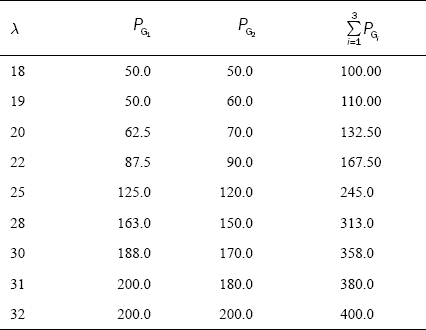
Example 2.10: Three power plants of a total capacity of 500 MW are scheduled for operation to supply a total system load of 350 MW. Find the optimum load scheduling if the plants have the following incremental cost characteristics and the generator constraints:
![]()
![]()
![]()
Solution:
For economic load scheduling among the power plants, the necessary condition is
![]()
For three plants,
![]()
Given total load = PG1 + PG2 + PG3 = 350 MW (2.34)
40 + 0.25 PG1 = 50 + 0.30 PG2 = 20 + 0.20 PG3 = λ (2.35)
![]()
⇒ 40 + 0.25 PG1 = 50 + 0.30 PG2
or 0.25 PG1 − 0.30 PG1 = 50 − 40 = 10 (2.36)
and 40 + 0.25 PG1 = 20 + 0.2 PG1
or 0.25 PG1 − 0.2 PG1 = 20 − 40 = −20 (2.37)
From Equation (2.36), we have

Substituting Equation (2.38) in Equation (2.34)
PG1 + 0.833 PG1 − 33.33 + PG3 = 350
or 1.833 PG1 + PG3 = 383.33 (2.39)
Solving Equations (2.37) and (2.39)
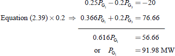
Substituting the value of PG1 in Equation (2.39),
1.833 × 91.98 + PG3 = 383.33 G3
or PG3 = 214.73 MW
Substituting the values of PG1 and PG2 in Equation (2.34), we get
91.98 + PG2 + 214.73 = 350
or PG2 = 43.29 MW
∴ For economic scheduling of the load, the generations of three plants must be
PG1 = 91.98 MW, PG2 = 43.29 MW, and PG3 = 214.73MW
Example 2.11: The fuel cost of two units are given by
C1 = 0.1 P2G1 = 25 PG1 + 1.6 Rs./hr
C2 = 0.1 P2G2 + 32 PG2 + 2.1 Rs./hr
If the total demand on the generators is 250 MW, find the economical load distribution of the two units.
Solution:
Given
![]()
![]()
Given the total load, PD = 250 MW. For economical distribution of total load, the condition is
![]()
0.2 PG1 + 25 = 0.2 PG2 + 32
or 0.2 PG1 − 0.2 PG2 = 7 (2.40)
and PG1 + PG2 = 250 (Given) (2.41)
By solving Equations (2.40) and (2.41), we get
2 PG1 = 285
or PG1 = 142.5 MW
Substituting the PG1 value in Equation (2.41), we get
PG2 = 250 − PG1 = 107.5 MW
Example 2.12: A plant has two generators supplying the plant bus, and neither is to operate below 20 or above 125 MW. Incremental costs of the two units are
![]()
![]()
For economic dispatch, find the plant cost of the received power in Rs./MWh (λ) when PG1 + PG2 equals: (a) 40 MW, (b) 100 MW, and (c) 225 MW.
Solution:
For economic operation,
![]()
(a) When PG1 + PG2 = 40 MW 2 (2.42)
![]()
0.15 PG1 − 20 = 0.225 PG2 + 17.5
or 0.15 PG1 − 0.225 PG2 = − 2.5 (2.43)
Equation (2.42) × 0.15 ⇒ 0.15 PG1 + 0.15 PG2 = 6.0 (2.44)
Solving Equations (2.43) and (2.44), we get
− 0.375 PG2 = − 8.5
PG2 = 22.66 MW
Substituting PG2 = 22.66 MW in Equation (2.42)
PG1 = 40 − 22.666
= 17.34 MW
![]()
0.225 PG2 + 17.5 = λ
or 0.225(226) + 17.5 = λ
∴ = 22.59 Rs./MWh
(b) When PG1 + PG2 = 100 MW (2.45)
Equation (2.45) × 0.15 ⇒ 0.15 PG1 + 0.15 PG1 = 15 (2.46)
By solving Equations (2.43) and (2.46), we get

Substituting the PG2 value in Equation (2.45), we get
PG1 = 53.34 MW
∴ 0.15 PG1 + 20 = λ or 0.225 PG2 + 17.5 = λ
0.15(53.34) + 20 = λ or λ = 0.225(46.66) + 17.5
⇒ λ = 28 Rs./MWh; λ = 28 Rs./MWh
(c) When PG1 + PG2 = 225 MW (2.47)
Equation (2.47) × 0.15 ⇒ − 0 15 PG1 + 0 15PG2 =33 75 (2.48)
By solving Equations (2.43) and (2.48), we get
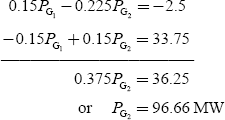
Substituting the PG2 value in Equation (2.47), we get
PG1 = 128.34 MW
∴ λ = 0.255 PG2 + 17.5
= 0.225(96.66) + 17.5
= 39.24 Rs./M Wh
Example 2.13: The cost curves of two generators may be approximated by second-degree polynomials:
C1 = 0.1 P2G1 + 20 PG1 + α1
C2 = 0.1 P2G2 + 30 PG2 + α2
where α1 and α2 are constants
If the total demand on the generators is 200 MW, find the optimum generator settings. How many rupees per hour would you lose if the generators were operated about 15% of the optimum settings?
Solution:
For economic operation,
![]()
0.2 PG1 + 20 = 0.2 PG2 + 30
or 0.2 PG1 + 0.2 PG2 = 10
or PG1 − PG2 = 50 (2.49)
and given that PG1 + PG2 = 200 (2.50)
Solving Equations (2.49) and (2.50), we get
2 PG1 = 250
or PG1 = 125 MW
Substituting the PG1 value in Equation (2.50), we get
PG2 = 200 – 125 = 75 MW
If the generators were operated about 15% of the optimum settings,
PG1 = 125 − 125 × ![]() = 125 − 18.75 = 106.25 MW
= 125 − 18.75 = 106.25 MW
and PG2 = 75 − ![]() = 75 − 11.25 = 63.75 MW
= 75 − 11.25 = 63.75 MW
The decrease in cost for Generator-1 is

The decrease in cost for Generator-2 is
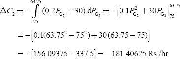
The loss of amount |
= |
ΔC1 − ΔC2 |
|
= |
− 58.59 − (− 181.40625) |
|
= |
− 122.81Rs./hr |
Example 2.14: Determine the saving in fuel cost in Rs./hr for the economic distribution of a total load of 225 MW between the two units with IFCs:
![]()
![]()
Compare with equal distribution of the same total load.
Solution:
Given: PG1 + PG2 = 225 MW (2.51)
For optimal operation:
![]()
⇒ 0.075 PG1 + 15 = 0.085 PG2 + 12
or 0.075 PG1 − 0.085 PG2= −3 (2.52)
Equation (2.51) × 0.085 ⇒ 0.085 PG1 + 0.285 PG2 = 225 × 0.085 = 19.125 (2.53)
By solving Equations (2.52) and (2.53), we get
0.16 PG1 = 16.125
or PG1 = 100.78 MW
Substituting the PG1 value in Equation (2.51), we get
PG2 = 225 – 100.78 = 124.218 MW
With equal distribution of the total load,
⇒ PG1 = 112.5 MW and PG2 = 112.5 MW
The increase in cost for Unit-1 is
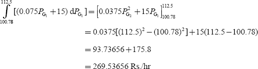
For Unit-2,

The negative sign indicates a decrease in cost.
∴ Saving in fuel cost = Rs. 269.53656 − 258.505
= 11.03156 Rs./hr
Example 2.15: Three plants of a total capacity of 500 MW are scheduled for operation to supply a total system load of 310 MW. Evaluate the optimum load scheduling if the plants have the following cost characteristics and the limitation:
C1 = 0.06 P2G1 + 30 PG1 + 10, 30 ≤ PG1 ≤ 150
C2 = 0.10 P2G2 + 40 PG2 + 15, 20 ≤ PG2 ≤ 100
C3 = 0.075 P2G3 + 10 PG3 + 20, 50 ≤ PG3 ≤ 250
Solution:
The IFCs of the three plants are
![]()
![]()

For optimum scheduling of units,
![]()
0.12PG1 + 30 = 0.20 PG2 + 40 = 0.15 PG3 + 10
![]()
⇒ 0.12 PG1 + 30 = 0.15 PG3 + 10
or PG1 − 0.15 PG2 = − 20 (2.54)
and given that PG1 + PG3 = 310 − PG2 (2.55)
Solving Equations (2.54) and (2.55), we have

or 0.27 PG1 + 0.15 PG2 = 26.5 (2.56)
and ![]()
0.12 PG1 + 30 = 0.2 PG2 + 40
0.12 PG1 − 0.2 PG2 = 10 (2.57)
Solving Equations (2.56) and (2.57), we get
Substituting the PG1 value in Equation (2.54), we get
0.12 (94.444) − 0.15 PG3 = − 20
11.33 − 0.15 PG3 = − 20
31.33 = 0.15 PG3
or PG3 = 208.86 MW
Substituting the PG1 and PG3 values in Equation (2.55), we get
94.44 + 208.86 + PG2 = 310
∴ PG2 = 6.7 MW
The optimal power generation is
PG1 = 94.44 MW
PG2 = 6.7 MW
and PG3 = 208.86 MW
It is observed that the real-power generation of Unit-2 is 6.7 MW and it is violating its minimum generation limit. Hence, we have to fix its value at its minimum generation, i.e., PG2 = 20 MW.
Given: PG1 + PG2 + PG3 = 310 MW
P1 + PG3 = 310 − 20 = 290 MW
The remaining load of 290 MW is to be distributed optimally between Unit-1 and Unit-3 as follows:
![]()
0.12 PG1 + 30 = 0.15 PG3 + 10
or 0.12 PG1 − 0.15 PG2 = − 20 (2.58)
and PG1 + PG3 = 290 (2.59)
Solving Equations (2.58) and (2.59), we get:
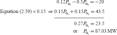
Substituting the PG1 value in Equation (2.59), we get
PG3 = 290 − 67.14 = 202.96 MW
The total load of 310 MW is distributed optimally among the units as
PG1 = 87.03 MW
PG2 = 20 MW
and PG3 = 202.96 MW
Example 2.16: The incremental cost characteristics of two thermal plants are given by
![]()
![]()
Calculate the sharing of a load of 200 MW for most economic operations. If the plants are rated 150 and 250 MW, respectively, what will be the saving in cost in Rs./hr in comparison to the loading in the same proportion to rating.
Solution:
For economic operation,
![]()
0.2 PG1 + 60 = 0.3 PG3 + 40
or 0.2 PG1 − 0.3 PG2 = − 20 (2.60)
or PG1 + PG2 = 200 (given) (2.61)
Solving Equations (2.60) and (2.61), we get
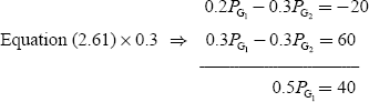
∴ PG1 = 80MW
Substituting the PG1 value in Equation (2.61), PG2 = 120 MW. If the plants are loaded in the same proportion to the rating,
i.e., PG1 = 150 MW, PG2 = 250 MW
Increase in the operation cost for Plant-1 is
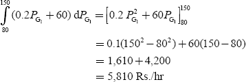
Increase in the operation cost for Plant-2 is

∴ Saving in operation cost = 12,415 − 5,810 = 66 Rs./hr
Example 2.17: The IFCs of two units in a generating station are as follows:
![]()
![]()
Assuming continuous running with a total load of 150 MW, calculate the saving per hour obtained by using the most economical division of load between the units as compared with loading each equally. The maximum and minimum operational loadings are the same for each unit and are 125 and 20 MW, respectively.
Solution:
Given: ![]()
![]()
Total load = PG1 + PG2 = 150 MW (2.62)
For optimality, ![]()
0.15 PG1 + 35 = 0.20 PG2 + 28
or 0.15 PG1 − 0.20 PG2 = −7 (2.63)
Solving Equations (2.62) and (2.63), we get
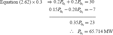
Substituting the PG1 value in Equation (2.62), we get
With an equal sharing of load, PG1 = 75 MW and PG2 = 75 MW.
With an equal distribution of load, the load on Plant-1 is increased from 65.714 to 75 MW.
The increase in cost of operation for Plant-1 is
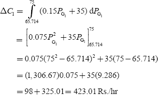
The load on Plant-2 is decreased from 84.286 to 75 MW.

∴ The solving in cost =423.01 − 407.921
= 15.089 Rs./hr
Example 2.18: If two plants having cost characteristics as given
C1 = 0.1 P2G1 + 60 PG1 + 135 Rs./hr
C1 = 0.15 P2G1 + 40 PG2 + 100 Rs./hr
have to meet the following daily load cycle:
0 to 6 hrs – 7 MW
18 to 24 hrs – 70 MW
find the economic schedule for the different load conditions. If a cost of Rs. 450 is involved in taking either plant out of services or to return to service, find whether it is more economical to keep both plants in service for the whole day or to remove one of them during light-load service.
Solution:

For 0–6 hr: Total load = 7 MW
i.e., PG1 + PG2 = 7 MW (2.64)
The condition for the optimal distribution of load is
![]()
0.2 PG1 + 60 = 0.3 PG2 + 40
0.2 PG1 − 0.3 PG2 = − 40 (2.65)
Solving Equations (2.64) and (2.65), we get
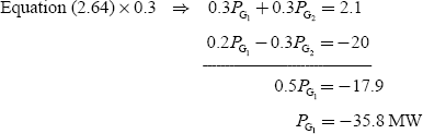
Since the real-power generation of Plant-1 is PG1 = — 35.8 MW, it violates the minimum generation limit. Hence, to meet the load demand of 7 MW, it is necessary to run Unit-2 only with generation of 7 MW.
Operation cost of Unit-2 during 0–6 hr is
C2 = 0.15(7)2 + 40(7) + 100
= 7.35 + 280 + 100
= 387.35 Rs./hr
For 18–24 hr:
Total load = 70 MW
i.e., PG1 + PG2 = 70 MW (2.66)
Solving Equations (2.66) and (2.65), we get
The cost of operation of Plant-1 with 2-MW generation is
C1 = 0.1PG1 + 60 PG1 + 135
= 0.1(2)2 + 60(2) + 135 = 255.4 Rs./hr
The cost of operation of Pant-2 with 68-MW generation is
C2 = 0.15(68)2 + 40(68) + 100 = 3,513.6 Rs./hr
The operating cost during 18–24 hr = 255.4 + 3,513.6 = 3,769 Rs./hr
The total operating cost during an entire 24-hr period is
387.35 × 6 + 3,769 × 6 = Rs. 24,938.10
A cost of Rs. 450 is incurred as the start-up cost.
∴ Total operating cost = 24,938.1 + 450 = Rs. 25,388.10
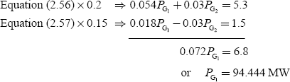
Example 2.19: The IFCs in rupees per MWh for a plant consisting of two units are
![]()
![]()
Calculate the extra cost increased in Rs./hr, if a load of 220 MW is scheduled as PG1 = PG2 = 110 M.
Solution:
For optimal scheduling of units,
![]()
0.20 PG1 + 40.0 = 0.25 PG2 + 30
or 0.20 PG1 − 0.25 PG2 = 10 (2.67)
Given: PG1 + PG2 = 220 (2.68)
Solving Equations (2.67) and (2.68), we get

Substituting the PG1 value in Equation (2.68), we get
∴ PG2 = 220 − PG1 = 120 MW
For an equal distribution of load,PG1 = 110 MW and PG2 = 110 MW. The operation cost of Unit-1 is increased as the load shared by it is increased from 100 to 110 MW.
∴ Increase in operation cost of Unit-1

The operation cost of Unit-2 is decreased as the load shared by it is decreased from 120 to 110 MW.
∴ Decrease in operation cost of Unit-2

The extra cost incurred in Rs./hr if the load is equally shared by Unit-1 and Unit-2 is
Example 2.20: The fuel cost characteristics of two generators are obtained as under:
C1 (PG1) = 1,000 + 50 PG1 + 0.01 P2G1 Rs./hr
C2 (PG2) = 2,500 + 45 PG2 + 0.005 P2G2 Rs./hr
If the total load supplied is 1,000 MW, find the optimal load division between two generators.
Solution:
C1 (PG1) = 1,000 + 50 PG1 + 0.01 P2G1 Rs./hr
C2 (PG2) = 2,500 + 45 PG2 + 0.005 P2G1 Rs./hr
The IFC characteristics are
![]()
![]()
The condition for optimal load division is
![]()
50 + 0.02 PG1 = 45 + 0.01 PG2
or 0.02PG1 + PG2 = − 5.0 (2.69)
PG1 + PG2 = 1,000 (given) (2.70)
Solving Equations (2.69) and (2.70), we get
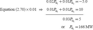
Substituting the PG1 value in Equation (2.70), we get
PG2 = 833 MW
Substituting the PG1 and PG1 values in ![]() equation, we get
equation, we get
λ = 53.33 Rs./MWh
∴ The total load of 1,000 MW optimally divided in between the two generators is
PG1 = 166 MW
PG2 = 833 MW
And IFC, λ = 53.33 Rs./MWh
Example 2.21: Determine the economic operation point for the three thermal units when delivering a total of 1,000 MW:
Unit A: |
Pmax = 600 MW, Pmin = 150 MW |
|
CA = 500 + 7 PGA + 0.0015 P2GA |
Unit B: |
Pmax = 500 MW, Pmin = 125 MW |
|
CB = 300 + 7.88 PGB + 0.002 P2GB |
Unit C: |
Pmax = 300 MW, Pmin = 75 MW |
|
CC = 80 + 7.99 PGC + 0.05 P2GC |
Fuel costs:
Unit A = 1.1 unit of price/MBtu
Unit B = 1.0 unit of price/MBtu
Unit C = 1.0 unit of price/MBtu
Find the values of PGA, PGB and PGC for optimal operation.
Solution:
Cost curves are:
CA (PGA) = HA × 1.1 = 550 + 7.7 PA + 0.00165 P2A
CB (PGB) = HB × 1.0 = 300 + 7.88 PB + 0.002 P2B
CC (PGC) = HC × 1.0 = 80 + 7.799 PC + 0.005 P2C
Now IFCs are:
![]()
![]()
![]()
For an economic system operation,
![]()
![]()
7.7 + 0.0033 PGA = 7.99 + 0.001 PG1
or 0.0033PGA − 0.01PGC = 0.29 (2.71)
PGA + PGB + PGC = 1, 000 (given)
or PGA = 1,000 − (PGB + PGC) (2.72)
Substituting PGA from Equation (2.72) in Equation (2.71), we get
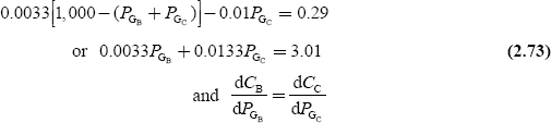
7.88 + 0.004 PGB = 7.99 + 0.01 PGC
or 0.004 PGB + 0.0133 PGC = 0.11 (2.74)

Substituting the PGB value in Equation (2.73), we get
0.0033(366.16) + 0.0133PGC = 3.01
or PGC = 135.464 MW
Substituting PGB and PGC values in Equation (2.72), we get
PGA = 498.376 MW
For a total load of 1,000 MW, the economic scheduling of three units are:
PGA = 498.376 MW |
(150 MW < PGA < 600 MW) |
PGB = 366.16 MW |
(125 MW < PGB < 500 MW) |
and PGC = 135.464 MW |
(75 MW < PGC < 300 MW) |
Example 2.22: The fuel cost curve of two generators are given as:
CA (PGA) = 800 + 45 PGA + 0.01 PGA
CB (PGB) = 200 + 43 PGB + 0.003 PGB
and if the total load supplied is 700 MW, find the optimal dispatch with and without considering the generator limits where the limits have been expressed as:
50 MW ≤ PGA ≤ 200 MW
50 MW ≤ PGB ≤ 600 MW
Compare the system’s increment at cost with and without generator limits considered.
Solution:
![]()
![]()
For economic operation, ICA = ICB = λ
Considering along with the given constraint equations:
λ |
= |
45 + 0.02 PGA |
λ |
= |
43 + 0.02 PGB |
PGA + PGB |
= |
700 MW |
Solving these equations,
λ =46.7
PGA = 84.6 MW
PGB = 615.4 MW
In the above illustration, generator limits have not been included. If these limits are now included, it may be seen that Generator-B has violated the limit. Fixing it at the uppermost limits, let
|
PGB |
= |
600 MW |
And obviously by so that |
PGA |
= |
100 MW (since PGA + PGB = 700 MW) |
∴ |
λA |
= |
45 + 0.02 × 100 = 47 |
|
λB |
= |
43 + 0.006 × 600 = 46.6 |
Hence, it is observed that λA ≠ λB, i.e., economic operation is not strictly maintained in this particular condition; incremental cost of Unit-A is now marginally more than that of Unit-B. However, in practice, this difference of λA and λB is not much; hence, the system operation is justified under this condition.
Example 2.23: The fuel cost curve of two generators are given as
C1 = 625 + 35 PG1 + 0.06 P2G1
C2 = 175 + 30 PG2 + 0.005 P2G1
if the total load supplied is 550 MW, find the optimal dispatch with and without considering the generator limits:
35 MW ≤ PG1 ≤ 175 MW
35 MW ≤ PG2 ≤ 600 MW
and also comment about the incremental cost of both cases.
Solution:
Given that total load = PG1 + PG2 = 550 MW (2.75)
Cost of first unit, C1 = 625 + 35 PG1 + 0.06P2G1
The IFC of first unit, ![]()
Cost of second unit, C2 = 175 + 30 PG2 + 0.005P2G2
The IFC of second unit, ![]()
Case-I: Without considering generator limits:
For optimal dispatch of load, the necessary condition is
![]()
0.12 PG1 + 35 = 0.01 PG2 + 30
0.12 PG2 + 0.01 PG2 = − 5 (2.76)
Solving Equations (2.75) and (2.76), we get
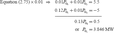
Substituting the PG1 value in Equation (2.75), we get
PG1 = 550 − 3.846 = 546.154 MW
The above results are for the case without considering the generator limits.
The IFCs are

The IFC, λ = 35.46 Rs./MWh
Case-II: Considering the generator limits:
35 MW ≤ PG1 ≤ 175 MW
30 MW ≤ PG2 ≤ 600 MW
From Case-I, the obtained power generations are
PG1 = 3.846 MW
PG2 = 546.154 MW
It is observed that the real-power generation of Unit-1 is violating the minimum generation limit. To achieve the optimum operation, fix up the generation of the first unit at its minimum generation, i.e.,PG1 = 35 MW. Hence, for the load of 550 MW, PG1 = 35 MW and PG2 = 550-35 = 515 MW.
Then, the IFCs are
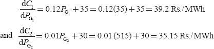
Hence, it is observed that λ1 ≠ λ2, i.e., economic operation is not strictly maintained in this particular condition.
Comment on the results: When the generator limits are not considered, the economic operation of generating units is obtained at an IFC of 33.45 Rs./MWh. Their economic operation is not obtained when considering the generation limits, since the IFC of the first unit is somewhat marginally greater than that of the second unit.
KEY NOTES
- Economic operation of a power system is important in order to maintain the cost of electrical energy supplied to a consumer at a reasonable value.
- In analyzing the economic operation of a thermal unit, input–output modeling characteristics are of great significance.
- For operational planning, daily operation, and for economic scheduling, the data normally required are as follows:
For each generator
- Maximum and minimum output capacities.
- Fixed and incremental heat rate.
- Minimum shutdown time.
- Minimum stable output.
- Maximum run-up and run-down rates.
For each station
- Cost and calorific value of the fuel.
- Factors reflecting recent operational performance of the station.
- Minimum time between loading and unloading.
For the system
- Load cycle.
- Specified constraints imposed on transmission system capability.
- Spare capacity requirement.
- Transmission system parameters including maximum capacities and reliability factors.
- To analyze the power system network, there is a need of knowing the system variables. They are:
- Scheduling is the process of allocation of generation among different generating units. Economic scheduling is the cost-effective mode of allocation of generation among the different units in such a way that the overall cost of generation should be minimum.
- Input–output characteristics establish the relationship between the energy input to the turbine and the energy output from the electrical generator.
- Incremental fuel cost is defined as the ratio of a small change in the input to the corresponding small change in the output.
- Incremental efficiency is defined as the reciprocal of incremental fuel rate.
- The input–output characteristics of hydro-power unit co-ordinates are water input or discharge (m3/s) versus output power (kW or MW).
Constraint Equations
The economic power system operation needs to satisfy the following types of constraints:
- Equality constraints.
- Inequality constraints.
(a) According to the nature:
- Hard-type constraints.
- Soft-type constraints.
(b) According to the power system parameters:
- Output power constraints.
- Voltage magnitude and phase-angle constraints.
- Transformer tap position/settings constraints.
- Transmission line constraints.
SHORT QUESTIONS AND ANSWERS
- Justify the production cost being considered as a function of real-power generation.
The production cost in the case of thermal and nuclear power stations is a function of fuel input. The real-power generation is a function of fuel input. Hence, the production cost would be a function of real-power generation.
- Give the expression for the objective function used for optimization of power system operation.

- State the equality and inequality constraints on the optimization of product cost of a power station.
The equality constraint is the sum of real-power generation of all the various units that must always be equal to the total real-power demand on the system.
The inequality constraint in each generating unit should not be operating above its rating or below some minimum generation.
i.e., PGi(min) ≤ PGi ≤ PGi (max),
for i = 1, 2, 3, …, n
- What is an incremental fuel cost and what are its units?
Incremental fuel cost is the cost of the rate of increase of fuel input with the increase in power input. Its unit is Rs./MWh.
- How is the inequality constraint considered in the determination of optimum allocation?
If one or several generators reach their limit values, the balance real-power demand, which is equal to the difference between the total demand and the sum of the limit value, is optimally distributed among the remaining units by applying the equal incremental fuel cost rule.
- On what factors does the choice of a computation method depend on the determination of optimum distribution of load among the units?
The factors depend upon the following:
- Number of generating units.
- The degree of polynomial representing the IC curve.
- The presence of discontinuities in the IC curves.
- What does the production cost of a power plant correspond to?
The production cost of a power plant corresponds to the least of minimum or optimum production costs of various combinations of units, which can supply a given real-power demand on the station.
- To get the solution to an optimization problem, what will we define an objective’s function?
Minimize the cost of production, min C′ = min C(PGn)
- Write the condition for optimality in allocating the total load demand among the various units.
The condition for optimality is the incremental fuel cost,

- Write the separable objective function and why it is called so.
The above objective function consists of a summation of terms in which each term is a function of a separate independent variable. Hence, it is called separable objective function.
- Briefly discuss the optimization problem.
Minimize the overall cost of production, which is subjected to equality constraints and inequality constraints.
Equality constraint is:

Inequality constraint is
PGi(min) ≤ PGi ≤ PGi(max)
- What is the reliable indicator of a country’s or state’s development?
It is the per capita consumption of electrical energy.
- State in words the condition for minimum fuel cost in a power system when losses are neglected.
The minimum fuel cost is obtained when the incremental fuel cost for all the stations is the same in the power system.
- What is the need of system variables and what are the variables?
To analyze the power system network, there is a need of knowing the system variables. They are:
- Control variables—PG and QG.
- Disturbance variables—PD and QD.
- State variables—V and δ.
- Define the control variables.
The real and reactive-power generations are called control variables since they are used to control the state of the system.
- Define the disturbance variables.
The real and reactive-power demands are called demand variables and they are beyond system control and are hence called uncontrolled or disturbance variables.
- (Define the state variables.
The bus voltage magnitude V and its phase angle δ dispatch the state of the system. They are dependent variables that are being controlled by the control variables.
- What is the need of input–output characteristics of a steam unit?
It establishes the relationship between the energy input to the turbine and the energy output from the electrical generator.
- Define the incremental fuel or heat rate curve.
It is defined as the ratio of a small change in the input to the corresponding small change in the output.
Incremental fuel rate
- How do you get incremental cost curve?
The incremental cost curve is obtained by considering at various points, the change in cost of generation to the change in real-power generation, i.e., slope of the input–output curve.
- How you get the heat rate characteristic?
The heat rate characteristic is obtained from the plot of net heat rate in kCal/kWh versus power output in kW.
- Define the incremental efficiency.
It is defined as the reciprocal of incremental fuel rate and is given by
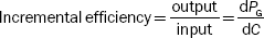
- What are hard-type constraints? Give examples.
Hard-type constraints are definite and specific in nature. No flexibility will be taken place in violating these types of constraints.
E.g., The tapping range of an on-load tap-changing transformer.
- What are soft-type constraints? Give examples.
Soft-type constraints have some flexibility with them in violating these type of constraints.
E.g., Magnitudes of node voltages and the phase angle between them.
- What is the need of spare capacity constraints?
These constraints are required to meet:
- Errors in load prediction.
- The unexpected and fast changes in load demand.
- Unplanned loss of scheduled generation, i.e., the forced outages of one or more alternators on the system.
MULTIPLE-CHOICE QUESTIONS
- In a thermal-electric generating plant, the overall efficiency is improved when:
- Boiler pressure is increased.
- The difference between initial pressure and temperature and exhaust pressure and temperature are held at a maximum.
- Load on the units is increased.
- Its operating time is increased.
- When load on a thermal unit is increased, fuel input:
- Increases.
- Does not change.
- Decreases.
- None of these.
- Incremental heat rate curves, for thermal generating units, are used to determine the:
- Fuel cost in rupees per hour.
- Values at which the units should be loaded to result in minimum fuel costs.
- Cost per unit of electrical output.
- Heat produced per hour.
- When generating units are loaded to equal incremental costs, it results in:
- Minimum fuel costs.
- Fuel costs are at a maximum.
- Fuel costs are not affected.
- Maximum loading of generating units.
- One advantage of computer control of generating units is that:
- Net output of the units is minimized.
- All units under the control of the computer will be loaded to the same load.
- Loading of the units will be frequently adjusted to maintain them at equal incremental costs.
- Both (b) and (c).
- If the fuel cost of one unit, operating in parallel with other units, is increased and it is desired to maintain average fuel cost, the load on the unit will be:
- Increased.
- Held constant.
- Decreased.
- None of these.
- In a power system using both hydro- and thermal-generation, the proportion of hydro-generation can be increased by:
- Increasing the price (gamma) of water.
- Reducing the price of water.
- Increasing the field currents of the hydro-generators.
- None of these.
- Economic operation of power system is:
- Unit commitment.
- Load scheduling.
- Controlling of voltage and its magnitude.
- Both (a) and (b).
- Lagrangian multiplier method converts a non-linear constrained optimization problem into _____ non-linear optimization problem.
- Gradient.
- Linear.
- Unconstrained.
- All of these.
- Unit of heat rate curve is _____.
- Million kCal/hr.
- Rs.-hr.
- Rs./MWh.
- Rs./hr.
- Power balance equation is _____ constraint.
- Equality.
- Inequality.
- Security constraints.
- Branch transfer capacity constraint.
- Optimization problems with only objective function and without constraints is a _____ function.
- Single-valued.
- Multi-valued.
- Both (a) and (b).
- Either (a) or (b).
- Unit of λ is _____.
- Rs./hr.
- Rs./MW.
- Rs./MWh.
- MW/Rs.
- Which of the following has a negligible effect on the production cost?
- Generation of real power.
- Real and reactive-power demands.
- System voltage and angle.
- Generation of reactive power.
- (i) and (ii).
- Except (iii).
- (ii) and (iv).
- All of these.
- An analytical method of getting the solution to optimization problem, the following graph is to be drawn:
- Total real-power demand versus λ.
- Total real-power generation versus total real- power demand.
- Total real-power generation versus λ.
- Total real-power generation versus fuel input.
- The control variables are:
- PD and QD.
- PG and QG.
- V and δ.
- Q and δ.
- PD and QD are:
- Control variables.
- State variables.
- Disturbance variables.
- Constants.
- PD and QD are:
- Disturbance variables.
- Demand variables.
- Uncontrollable variables.
- All of these.
- Cost curves can be obtained by:
- Multiply the fuel input with cost of fuel.
- Subtract the fuel input with cost of fuel.
- Add the fuel input with cost of fuel.
- None of these.
- Cost curves are expressed as:
- Rs./million cal.
- Million cal/hr × Rs./million cal.
- Rs./hr.
- (b) and (c).
- The curve obtained by considering the change in cost of generation to change in real-power generation at various points is:
- Fuel cost curve.
- Input–output curve.
- Incremental cost curve.
- All of these.
- Incremental fuel cost, IC is given by:
- Rs./MWh.
- Slope of the fuel cost curve.
- Tan β = ∆C/∆PG.
- ∆i/p/∆o/p.
- (i) and (ii).
- (ii) and (iii).
- All except (iv).
- All of these.
- Incremental production cost of a given unit is made up of:
- IC - incremental cost of labor, supplies, maintenance, etc.
- IC + incremental cost of labor, supplies, maintenance, etc.
- IC × incremental cost of labor, supplies, maintenance, etc.
- IC% incremental cost of labor, supplies, maintenance, etc.
- The optimization problem is:
- To allocate total load demand among various units such that the cost of generation is maintained constant.
- To allocate total load demand among various units such that the cost of generation is minimized.
- To allocate total load demand among various units such that the cost of generation is enormously increased.
- To allocate total load demand among various units such that there is no effect with cost of generation.
- The method adopted to get an optimal solution to optimal scheduling problem depends on:
- The mathematical equation representing IC.
- No. of units.
- Need to represent any discontinuity in incremental cost curve.
- Change in location.
- Only (i).
- Only (ii).
- All expect (iv).
- All expect (ii).
- In a digital computer method of getting the solution to an optimization problem,
- The number of terms included in expression for
 depends on the degree of accuracy.
 - α, β, γ coefficients are to be taken
as output. - α, β, γ coefficients are to be taken as input.
- Both (i) and (ii).
- Both (i) and (iii).
- Only (i).
- Only (iii).
- The number of terms included in expression for
- If the real-power inequality constraints are violated for any generator, then:
- It is tied to the corresponding limit and the rest of the load is economically distributed among the remaining units.
- It is tied to the corresponding limit and the total load is economically distributed among all the units.
- It is not considered and the total load is economically distributed among all the units.
- Any of the above methods.
- The method of getting the solution to an optimization problem with neglected transmission losses:
- To get an optimal solution to an optimization problem, we will define an objective function as:
- The condition for optimality is:
 .
. .
. .
.- (d) Both (a) and (b).
- Which of the following is the real indicator of the state of development of a country?
- Population.
- Facilities.
- Politics.
- Per capita consumption of electricity.
- Equality and inequality constraints are
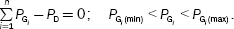
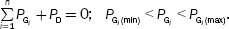

- (d) None of the above.
- In a mathematical determination, the optimization problem should be modified as:
- Constrained optimization problem.
- Normalized optimization problem.
- Conditional optimization problem.
- All the above.
REVIEW QUESTIONS
- Explain the important characteristics of a steam unit.
- Describe the need of economic dispatch.
- Explain why the production cost of electrical energy is treated as a function of real-power generation.
- Obtain the condition for optimum operation of a power system with ‘n’ plants.
- Bring out the difference between optimal operation of generators in thermal stations and optimal scheduling of hydro-thermal systems.
- Explain how the incremental production cost of a thermal power station can be determined.
- Explain the various factors to be considered in allocating generation to different power stations for optimum operation.
- Explain the significance of equality and inequality constraints in the economic allocation of generation among different plants in a system.
PROBLEMS
- Three power plants of a total capacity of 425 MW are scheduled for operation to supply a total system load of 300 MW. Find the optimum load scheduling if the plants have the following incremental cost characteristics and the generator constraints.

- A plant consists of two units. The incremental fuel characteristics for the two units are given as:
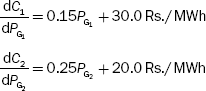
Find the optimal load sharing of two units when a total load of 300 MW is connected to the system. Also calculate the extra cost increased in Rs./hr if the total load is shared equally between them.
- The cost curves of the three plants are given as follows:
C1 = 0.04 P2G1 + 20 PG1 + 230 Rs./hr
C2 = 0.06 P2G2 + 18 PG2 + 200 Rs./hr
C3 = 0.05 P2G3 + 15 PG3 + 180 Rs./hr
Determine the optimum sharing of a total load of 180 MW for which each plant would take up for minimum input cost of received power in Rs/MWh.
- The incremental fuel costs in rupees per MWh for a plant consisting of two units are:
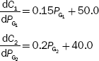
Calculate the extra cost increased in Rs./hr, if a load of 210 MW is scheduled as PG1 = PG2 = 105 MW.