13

Power System Security and State Estimation

13.1 INTRODUCTION

The concept of control is fundamental to the proper functioning of any system. Irrespective of whether it is an engineering system or an economic system or a social system, it is essential to exert some kind of control, such as quality control, inventory control, or population control, to achieve certain objectives like better quality of output or better economics, etc. It is only natural that power system, which is one of the most complex man-made systems, calls for the implementation of a number of controls for satisfactory operation. Power system control has gone through a lot of changes over the past three decades. Beginning with simple governor control at the machine level, it has now grown into a sophisticated multilevel control needing, a real-time computer process, and system-wide instrumentation.

The ultimate objective of power system control is to maintain continuous electric supply of acceptable quality by taking suitable measures against the various disturbances that occur in the system. These disturbances can be classified into two major heads, namely, small-scale disturbances and large-scale disturbances. Small-scale disturbances comprise slowly varying small-magnitude changes occurring in the active and reactive demands of the system. Large-scale disturbances are sudden, large-magnitude changes in system operating conditions such as faults on transmission network, tripping of a large generating unit or sudden connection or removal of large blocks of demand. While the small-scale disturbances can be overcome by regulatory controls using governors and exciters, the large-scale disturbances can only be overcome by proper planning and adopting emergency switching controls.

13.2 THE CONCEPT OF SYSTEM SECURITY

‘Security control’ or a ‘security control system’ may be defined as a system of integrated automatic and manual controls for the maintenance of electric power service under all conditions of operation. It may be noted from this definition that security control is a significant departure from the conventional generation control or supervisory control systems. First, the proper integration of all the necessary automatic and manual control functions requires a total systems approach with the human operator being an integral part of the control system design. Second, the mission of security control is all-encompassing, recognizing that control decisions by the main computer system must be made not only when the power system is operating normally but also when it is operating under abnormal conditions. As power systems have become more tightly coupled, the problem of making the operating decisions under varying conditions has become extremely difficult.

To keep the system always secure, it is necessary to perform a number of security-related studies, which can be grouped into three major areas, namely, long-term planning, operational planning, and on-line operation.

Certain significant applications in each of these areas are listed as follows:

13.2.1 Long-term planning

• Evaluation of generation capacity requirements.
• Evaluation of interconnected system power exchange capabilities.
• Evaluation of transmission system adequacy.

13.2.2 Operational planning

• Determination of spinning reserve requirements in the unit commitment process.
• Scheduling of hourly generation as well as interchange scheduling among neighboring systems.
• Outage dispatching of transmission lines and transformers for maintenance and system operation.

13.2.3 On-line operation

• Monitoring and estimation of the operating state of the system.
• Evaluation of steady-state, transient, and dynamic securities.
• Quantitative assessment of security indices.
• Security enhancement through constrained optimization.

13.3 SECURITY ANALYSIS

Security analysis is the determination of the a security of the system based on a next-contingency set. This involves verifying the existence and normalcy of the post-contingency states. If all the post-contingency states exist and are found to be normal, the state is secure. On the other hand, the non-existence of even one of the post-contingency states or emergency nature of an existing post-contingency state indicates that the current state is insecure.

Though it may be theoretically possible to conduct a security analysis for both the steady-state emergency and dynamic instability, the trend has been to have a separate analysis for each of these two types of emergency. The main reason for this is the extreme difficulty in implementing a dynamic-security analysis with the present methods of stability analysis. On the other hand, for the steady-state security (SSS) analysis, several approaches are possible and are in use. Basically, these approaches start with a knowledge of the present state of the system as obtained from the security monitoring function. The system is then tested for various next-contingencies by, in effect, solving for the changes in the system conditions for a given contingency and checking the new values against the operating constraints.

‘Transient security analysis’ refers to an on-line procedure whose objective is to determine whether or not a postulated disturbance will cause transient instability of the power system. A transient instability condition implies the loss of synchronism or oscillations, which increase in amplitude, leading to cascading outages and subsequent system breakup. As against the SSS analysis where the next-contingencies to be considered are only outages of lines/transformers or generators, in the case of transient security analysis, a much wider range of possible contingencies must be considered such as:

• Single-phase, two-phase, and three-phase fault conditions.
• Faults with or without reclosing.
• Proper operation or failure of protective relays.
• Circuit breaker operation or failure to clear the fault.
• Loss of generation or a large block of load.

Direct methods for transient security analysis have been suggested, but none of these have yet passed the experimental stage. The current industry practice is to express the security constraints associated with transient stability as steady-state operating limits on power transfer or phase-angle difference across selected transmission lines. The general approach for imposing transient security constraints on an operating power system consists of the following steps:

1. Perform extensive off-line transient stability studies for a range of operating conditions and postulated contingencies.
2. On the basis of these studies and pre-determined reliability criteria (e.g., the system must withstand three-phase faults with normal clearing), establish steady-state operating limits for line power flows or line phase-angle differences.
3. Operate the system within the constraints determined in the previous step.

Transient stability analysis of a large system, though done using a crude machine model of constant emf behind transient reactance, requires quite a lot of computer time because of the large number of differential algebraic equations involved. When one goes for a model of higher degree of complexity, which may include an excitation system model, detailed generator electrical model, governor control model, and turbine model and if one considers simulation for each of the contingencies in the next-contingency set, then the computation time needed becomes prohibitive. In recent years, considerable amount of research has been devoted to developing efficient and effective techniques for on-line transient stability analysis. The suggested techniques can be classified according to the following basic approaches:

1. Digital simulation.
2. Hybrid computer simulation.
3. Lyapunov methods.
4. Pattern recognition.

13.3.1 Digital simulation

Digital simulation techniques, though very adaptable and flexible, are slow in speed and hence it appears that they will use on-line analysis in a complementary role with faster, but possibly less accurate, techniques. Recent advances in digital methods have been directed toward implicit integration techniques and the simultaneous solution of the whole set of differential-algebraic equations using sparsity techniques. It is claimed that a method like ‘variable integration step transient analysis’ (VISTA) can reduce the simulation time as much as five times as compared with the conventional explicit integration methods.

13.3.2 Hybrid computer simulation

Hybrid computer simulation of a transient stability problem could be made many times faster than real time. Although hybrid computers have been able to provide matchless solution speeds, their application to power system operation is limited by disadvantages such as very large initial investment in the case of large systems; applicable only to a limited number of select on-line computation functions and limited flexibility due to the normal patching of the analog computers.

13.3.3 Lyapunov methods

The second method of Lyapunov has received a considerable amount of attention for determining power system transient stability, particularly for on-line application. This method involves the derivation of a scalar Lyapunov V(X), where X is the dynamic-state vector of the system set of differential equations, which has the following properties:

    V(0) = 0,    i.e., X = 0 is the equilibrium state

    V(X) > 0,   X ∈ Ω, X ≠ 0

    V(X) ≤ 0,   X ∈ Ω

where Ω is a region around the stable point X = 0, which is called the region of stability. While this method can offer considerable gain in computational speed, the drawbacks of this method as follows are:

• Too conservative, especially for systems with more than three or four machines.
• Computational requirements have made the study of large-scale power systems infeasible.
• Requires a simplified system model.

The last limitation is not as severe as the first two since much useful information can be obtained from analytical studies with the simplified models. Very recent developments indicate that a breakthrough in overcoming the first two problems is now possible. First, an efficient method of calculating the unstable equilibrium point has been developed using a modified Newton-Raphson load flow. Second, there is now an increased amount of awareness as to why the second method of Lyapunov is highly conservative.

13.3.4 Pattern recognition

Pattern recognition is another approach aimed at overcoming the high computational requirements of on-line transient stability studies. A large number of off-line stability studies are performed to form a ‘training set’ and certain important features are selected. An on-line classifier compares the actual operating conditions with the training set and, on the basis of this comparison, classifies the existing state as either secure or insecure. This method is very appealing for on-line assessment because of its tremendous speed and the minimum on-line data that it requires.

However, the disadvantages of this method are:

1. The accuracy of the classification method is not as good as that of the direct solution methods since it is basically an interpolation technique.
2. A very large number of samples (and hence simulation) may be required for the formation of an adequate training set.
3. It has difficulty in handling abnormal conditions, which may arise due to unusual load patterns and/or network configurations.

If the duration of the analysis to be conducted is longer than 1–3 s, the dynamics of the boilers, turbines, and other power plant components cannot be ignored. In addition to this, the dynamics of AGC and SVC should be taken into account along with the control action of impedance and under-frequency load-shedding relays. As a result, the effect of a fault-initiated disturbance may continue past the transient stability phase to the so-called long-term dynamic stability phase, which can be of the order of 10–20 min or more. The objectives of a long-term dynamic response assessment are:

1. Evaluation of dynamic reserve response characteristics including the distribution of reserves and effect of fast-starting units.
2. Evaluation of emergency control strategies like load-shedding by under-frequency relays, fast valuing, dynamic braking, and others.

These objectives fall primarily under system planning, control system design, as well as post-disturbance analysis. However, the operating implications cannot be neglected, in view of the fact that serious blackouts that have occurred over the past 15–20 years were generally the result of long-term instability and sequences of cascading events.

13.4 SECURITY ENHANCEMENT

Security enhancement is a logical adjunct to security analysis and it involves on-line decisions aimed at improving (or maintaining) the level of security of a power system in operation. Security enhancement includes a collection of control actions, each aimed at the elimination of security constraint violations. These controls may be classified as:

1. Preventive controls in the normal operating state, when on-line security analysis has detected an insecure condition with respect to a postulated next-contingency.
2. Correctable emergency controls (simply called ‘corrective controls’) in an emergency state, when an out-of-bound operating condition already exists but may be tolerated for a limited time period.

In either case, the primary objective is to find feasible and practical ways to remedy a potentially dangerous operating condition once the security analysis program reveals the existence of such a condition.

Security enhancement implies the utilization of available generation and transmission capacity to improve the security of a power system. There are five generic approaches to the use of available system resources for security enhancement, namely:

1. Manipulation of real-power flows in certain parts of the system through rescheduling of generation along with other control variables such as phase-shifter ratios.
2. Manipulation of reactive-power flows in the system to maintain a good ‘voltage profile’ through excitation control of generators along with other control variables such as shunt capacitor or reactor switching, off-nominal tap ratios of transformers, etc.
3. Utilizing heat capacity of components like transformers and underground cables to permit short-term overloading of certain pieces of equipment.
4. Changing the network topology via switching actions.
5. Modifying the settings of protective relays or control logic.

All the five options given above involve some trade-offs between the economy and the security of power system operation. For example, generation shifting or rescheduling power transactions usually result in higher operating costs. Hence, for those preventive control actions that drastically affect the economy of operation, the operator may decide not to execute the recommended control actions until the postulated contingency actually takes place, depending on the general operating philosophy of the particular system and the nature of the predicated constraint violations.

Security-constrained optimization may be used as a convenient framework for discussing approaches to system security enhancement, especially for SSS. The constrained optimization problem of obtaining the ‘best’ operating condition that satisfies not only the load constraints and the operating constraints but also the security constraints may be stated as follows:

Minimize

f (X, U) objective function

Subject to:

G(X, U) = 0, load constraints

H(X, U) ≥ 0, operating constraints

S(X, U) ≤ 0, security constraints

where f is a scalar-valued function.

The security constraints reflect all the operating and load constraints associated with the postulated post-contingency states; these ‘logical constraints’ can be rigorously formulated and expressed as a set of inequality constraints as indicated above. These functional constraints, too large in number, make the problem very complex. Two non-linear programming techniques, namely the penalty function technique and the generalized reduced gradient technique, have been identified as most suitable for solving the constrained optimization problem. For a quick on-line solution, the dual linear programming technique using the linear model as well as the successive linear programming technique using linearized models have been found to be most useful.

Only a limited amount of research has been directed at the development of control algorithms for transient security enhancement. Since on-line implementation of control algorithms to enhance system security is very difficult to achieve, one can consider the intermediate step of computing and presenting suitable security indices to the operators who will in turn take control decisions. A number of security indices, both for SSS as well as for transient security, have been proposed along with a suitable technique of obtaining them from the on-line security analysis.

13.5 SSS ANALYSIS

Though SSS analysis is only a part of the overall security assessment process, its importance should not be underestimated. The reasons for its prominence are: first, it is the only simple simulation process that can be implemented on-line. It should be noted that at this time of writing when on-line security analysis is not yet in common use, except for a few pioneering applications, the SSS analysis is either in the early stages of on-line implementation or planned for several new energy control centers in developed countries. Second, it is advantageous to know whether (or not) the post-contingency state of the system would be acceptable from steady-state considerations, even before investigating the transient and dynamic performance. Third, an approximate check of transient stability could also be incorporated by imposing on the post-contingency steady states, appropriate power flow, or other constraints derived from off-line transient stability studies. Hence, it is logical to devote more attention on the various aspects of the SSS analysis.

The objective of the SSS analysis is to determine whether, following a postulated disturbance, there exists a new steady-state operating point where the perturbed power system will settle after the post-fault dynamic oscillations have been damped out. An on-line algorithm simulates the predicted steady-state conditions for a specified set of next-contingencies and checks for operating constraint violations. If the normal system fails to pass any one of the contingency tests, it is declared to be ‘steady-state insecure’ and the particular contingencies with the attendant limit excursions are noted. More precisely, SSS is defined as the ability of the system to operate steady-state-wise within the specified limits of safety and supply quality following a contingency, in the time period after the fast-acting automatic control devices have restored the system load balance, but before the slow-acting controls, e.g., transformer tapings and human decisions, have responded.

13.5.1 Requirements of an SSS assessor

The SSS assessor is defined as an on-line process using real-time data for conducting SSS analysis on the current state of the system. Each contingency is solved approximately as a steady-state AC power flow problem. Except for simulated outages, the network is the same as the actual operating system and the bus power injection (defined as generation minus load) schedule corresponds to the currently estimated state of the system. The results of each solution are checked against pre-determined constraints. If a contingency causes a constraint violation or if a solution for a contingency is impossible, this information is transferred from the SSS assessor to another function in the control center in which appropriate control actions will be taken to enhance the security of the system.

The SSS assessor will be one of several interrelated programs in an automated dispatch center. The ways in which it can be integrated with other functions are not considered here. However, a simplified schematic diagram for the flow of information is shown in Fig. 13.1. The most critical input is the state vector from the state estimator. This estimate is transmitted in the form of the state vector V consisting of complex voltages at each node of the monitored system.

Other essential inputs are explained as follows.

13.5.1.1 Network Data

The passive network is modeled by the bus admittance matrix [], which is developed from a detailed list of basic network components including transmission lines, transformers, capacitors, and reactors. It is essential to have real-time information on the status of these components at the beginning of each solution cycle. A solution cycle is the solution and checking of results for all contingent outages in a specified contingency list. The change of status of every network component is transmitted to the control computer and whenever a component is switched in or out, its effect is reflected by a change in the admittance matrix.

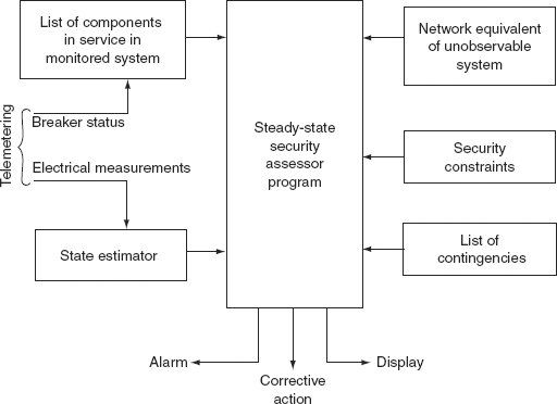
FIG. 13.1 Flow of information in a security assessor

13.5.1.2 Bus Power Injections

For a line outage, the injections should correspond to the actual state of the system. The injection schedule is computed once at the beginning of each solution cycle based on the network admittances and the state vector. The injection at every bus k is computed as

where P_k and Q_k are the real and reactive powers, and are elements of the state vector is an element of the bus admittance matrix [], and α _k is the set of all nodes adjacent to node k.

For physical as well as mathematical reasons, it is necessary to fix the voltage angle at the slack bus and allow the variation in losses to be supplied by the injection at this bus.

13.5.1.3 Security Constraints

The constraints are transmission line power flows, bus voltages, and reactive limits. These constraints may originate from customer requirements, relay settings, insulation levels, equipment ratings, or other sources. Constraints can also be established by off-line simulation studies. Line flow constraints are usually expressed either in terms of maximum continuous current or power ratings (normally for shorter lines), or in terms of the allowable maximum steady-state phase-single differences between connected buses (normally for longer lines). As stated earlier, SSS constraints can be derived to suit transient stability requirements. However, these constraints are difficult to specify, since the transient stability properties of a line depend on: the generation / load pattern throughout the entire network, the precise nature of the contingency, the configuration of the post-fault system, etc.

In some systems, it may be desirable to alter the constraints according to the state of the system, with different constraints applying under different operating conditions or contingencies. Establishing appropriate constraints for the SSS assessor is an important sub-problem that requires more investigation.

13.5.1.4 Contingency List

For the purpose of SSS analysis, the following contingencies should be considered:

1. Loss of a generating unit.
2. Sudden loss of a load.
3. Sudden change in flow in an inter-tie.
4. Outage of a transmission line.
5. Outage of a transformer.
6. Outage of a shunt capacitor or reactor.

These outages can be grouped into two categories: ‘network outage’ and ‘power outage’. A network outage involves only changes in the network admittance parameters and includes items (iv) to (vi) given above. A power outage involves only changes in bus power injections and hence includes items (i) to (iii) given above.

The usual practice in SSS analysis is to assume that the network configuration and the injection schedule at the contingency state remain the same as in the base case state except for the simulated outages. However, in dealing with power outages that involve the loss of certain generating units, the injection schedule at the contingency state should take into account the redistribution of lost generation to the remaining generators in service. This may be done with the help of a generation allocation function. Since the analysis is concerned with the new study after the outage transients have settled, the generation allocation will be determined by the natural governor characteristics of the available units in the system. However, if it is required to check the power flows immediately after the outage, then all the remaining generators in the system will share, temporarily, the lost generation in proportion to their inertias.

13.6 TRANSIENT SECURITY ANALYSIS

In recent years, a considerable amount of research has been devoted to developing efficient and effective techniques for on-line transient stability analysis. Transient stability assessment consists of determining if the system’s oscillations following a short-circuit fault will cause loss of synchronism among generators. The primary physical phenomenon involved here is that of inertial interaction among the generators as governed by the transmission network and busloads. This phenomenon is of short duration (1–3 s) in general. For longer durations, the dynamics of boilers, turbines, and other power plant components cannot be ignored. The suggested techniques to solve transient stability problems can be classified according to the following basic approaches:

1. Digital simulation.
2. Pattern recognition.
3. Lyapunov method.
4. Hybrid computer simulation.

13.6.1 Digital simulation

Several numerical integration approaches have been proposed and used. As in all integration schemes, the usual limiting factor is the smallest time constant of the system, which is normally caused by synchronizing oscillations. The use of implicit predictor-corrector methods has generally allowed larger step sizes while maintaining a high level of numerical stability. Normally, the transient stability program will alternate between an integration step and a load flow solution to solve the network equations. Thus, sparse matrix methods can be quite effective and useful in this context.

13.6.2 Pattern recognition

It is another approach aimed at overcoming the high computational requirements of online transient stability solutions. A large number of off-line stability studies are performed to form a ‘training set’ and certain important features are selected. An on-line classifier compares the actual operating conditions with the training set and, on the basis of this comparison, classifies the existing system as either secure or insecure. Consequently, the bulk of the computation load is transferred to the off-line studies’ time frame. This method leads to the generation of a function known as a ‘security function’, which is used to assess the security of the system.

13.6.3 Lyapunov method

The second method of Lyapunov has received considerable attention for determining power system transient stability, particularly for on-line application. However, the results of this research have been of little practical value to date, due to three basic problems. The classical Lyapunov method yields sufficient but not necessary conditions for stability; these conditions are discussed in detail in the following sections.

13.7 STATE ESTIMATION

The state of a power system is defined in terms of the voltage magnitude and phase angle of every bus in the power system. The state estimation plays a very vital role in power system operation, monitoring and control in terms of avoiding system failures and regional blackouts. The main objective of state estimation is to obtain the best possible values of the magnitudes of bus voltages and their angles and it requires the measurement of electrical quantities, such as real and reactive-power flows in transmission lines and real and reactive-power injections at the buses.

State estimation is an available data processing scheme to find the best state vectors, using the weighted least square method to fit a scatter of data. In order to obtain a higher degree of accuracy of the solution of the state estimation technique, two modifications are introduced. First, it is recognized that the numerical values of the available data to be processes for the state estimation are generally noisy due to the presence of errors. Second, it is noted that there are a large number of variables in the system (active and reactive-power line flows), which can be measured but not utilized in the load flow analysis. Thus, the process involves imperfect measurements that are redundant and the process of system state estimation is based on a statistical criterion that estimates the true values of the state variables either to minimize or maximize the selected criterion. A commonly used criterion is that of minimizing the sum of the squares of the differences between the estimated and measured true values of a function.

All the system information is collected by the centralized automation control of power system dispatch through remote terminal units (RTUs). The RTUs sample the analog variables and convert them into a digital form. These digital signals are interrogated periodically for the latest values and are transmitted by telephone and microwave communication link to the control center.

The control center operation must depend on measurements that are incomplete, inaccurate, delayed, and unreliable. The state estimation technique is used to process all the available data and hence the best possible estimate of the true value of the system is found.

13.7.1 State estimator

It processes real-time system data, which is redundant and computes the magnitudes of bus voltages and bus voltage phase angles with the help of a computer program. The inputs to an estimator are imperfect (noisy) power system measurements. It is designed to give the best estimate of system state variables (i.e., bus voltage magnitudes and phase angles).

The state estimator detects bad or inaccurate data by using statistical techniques. For this, state estimators are designed such that they have well-defined error limits and are based on the number, types, and accuracy of measurements.

The state estimator approximates the power flows and voltages at a bus whose measurements are not available because of RTU failure or breakdown of telephone or a communication link. Under such a condition, the state estimator is required to make available a set of measurements to replace missing or defective data.

13.7.2 Static-state estimation

There are two different modes of state estimation as applied to power systems:

1. Static-state estimation.
2. Dynamic-state estimation.

Static-state estimation pertains to the estimation of a system state frozen at a particular point in time. Figuratively speaking, it is a snapshot of the system. In the steady-state operation of a system (e.g., the sudden opening of one of the phases of a transmission line is reflected in the power flow in the two healthy phases much lesser than the average power flow indicated by the last-state estimation), the state estimator is required to detect a change in network configuration and convey a signal indicating the change in circuit configuration and to prepare the operator for corrective action on the first data scan. On the other hand, dynamic-state estimation is a continuous process, which takes into account the dynamics of the system and gives an estimate of the system state as it evolves in time. At the present moment, most of the state estimators in power systems, which are operational, belong to the first category.

On the face of it, it may appear as if there is not much of a difference between load flow calculations and static-state estimation. But, this is a superficial point of view. In load flow studies, it is taken for granted that the date on which calculations are based are absolutely free from error. On the other hand, in state-estimation methods, accuracy of measurement on modeling errors are taken into account by ensuring redundancy of input data. This means that the number of input data ‘m’ on which calculations are based are much more than the number of unknown variables ‘n’ whose knowledge completely specifies the system. The more the redundancy, the better it is from an estimation point of view. But redundancy has a price to pay in terms of installation of additional measuring equipment and communication facilities.

13.7.3 Modeling of uncertainty

From a mathematical viewpoint, the simplest way of describing a random vector ‘v’ is by assigning a Gaussian distribution to it. The probability density function for ‘v’ is then given by

Here, the expected value of v is assumed to be zero and R denotes the covariance matrix of v. The random vector v represents the following errors:

1. Instrumentation errors (meter errors, incomplete instrumentation, and bad data).
2. Operational uncertainties (unexpected system changes, measurement delay).
3. Incompleteness of the mathematical model (modeling errors, inaccuracy in network parameters).

13.7.4 Some basic facts of state estimation

There are three important quantities of interest in state estimation. They are:

1. The variable to be estimated.
2. The observations.
3. The mathematical model showing how the observations are related to the variables of interest (which are to be estimated) and the ever-present uncertainties.

The variables to be estimated are the state variables x, the observations are represented by z, and the mathematical model is given by

 

 

In Equation (13.3), ‘h’ represents a known non-linear relation connecting z and x. For pedagogical reasons, the above quantities are represented specifically as

 

x_true = true value of state x

z_actual = actual value of observation

v_actual = actual value of observation uncertainty

 

Further, for simplicity of explanation, let us assume that the non-linear relation in Equation (13.3) is replaced by a linear relation viz.,

 

 

where

In Equation (13.4), we know that

We note that even though x_true and v_actual are not known, the mathematical model conveys some information on their values, i.e., there is a model for their uncertainty. Now define:

 

: estimate of value x_true

The estimate depends on the value z and the mathematical model (and the uncertainty models for x_true and v_actual). Usually, it is desirable to view the estimate as some specified function of the observation z_actual. This function is called an estimator. The nature of this estimator can be determined from h and the models of x_true and v_actual. It can therefore be specified before observations are actually made. The estimator for linear systems is often a linear matrix operator W.

 

 

In general, is not equal to x_true. Hence, the first problem is to choose the best estimator (the best W), which minimizes, in some sense, the error (x_true − ). Assuming that such a W has been chosen, the second problem is to determine how close is to x_true. Since the numerical value of the error (x_true − ) is not known, the problem is to develop an uncertainty model for the same. The uncertainty in (x_true − ) depends upon h, the uncertainty in x_true and v_actual and of course the estimator W. Hence, in general terms, the basic estimation problem involves the following steps:

1. Find the estimator W
   
   such that is as close to x_true as possible.
2. Determine the model for the uncertainty in (x_ture − ). This model depends on the chosen W.

There are two models for the uncertainty x_true and they are:

1. A priori model: The model for x_true, which models the uncertainty before the observation is made.
2. A posteriori model: It is the model for (x_true−), which models the uncertainty in x_true after the observation has been made and processed to yield .

The choice of estimator such as W depends on the a priori model. The a posteriori model depends on which estimator W is chosen. In what is to follow, we drop the notation x_true and z_actual in favor of x and z.

There are many ways of modeling the uncertainty of x and v. Some of the more important ways are:

 

(i) Bayesian model	:	x and v are random vectors.
(ii) Fisher model	:	x is completely unknown; ‘v’ is random vector.
(iii) Weighted least squares	:	No models for x and v.
(iv) Unknown but bounded	:	x and v are constrained to lie in specified sets.

13.7.5 Least squares estimation

Consider the relation:

z = h(x) + v

or     v = [z − h(x)]                 (13.6)

and from Equation (13.2),

The optimal estimate is given by that value of x for which the scalar function of the weighted squares:

 

 

has a minimum value. The weighting matrix R⁻¹ is the inverse of the covariance matrix of the observation noise v.

Applying the first-order necessary conditions for minimizing J, we have

The second partial derivative of J with resect to ‘x’ viz., is a matrix known as the Hessian matrix and is denoted here by G(x):

The second-order sufficiency condition demands that G(x) be positive, definite at the minimum.

As usual in such problems, we follow the iterative procedure to successively close in on the minimum point , which in this case, is the least square estimate.

Therefore, assume the iterative form:

 

 

As k tends to infinity, hopefully x_k → x_{k + 1} and A_k g(x_k) → 0, which implies for non-singular A_k that g(x_k) = 0. This is precisely the condition to be satisfied by Equation (13.8) and hence the desired result is obtained.

There are several methods to arrive at the matrix A_k. A_k is a scalar multiple of unit matrix in the steepest descent method; it is the inverse of the Hessian matrix G(x_k) in Newton’s method. It is possible to choose A_k by taking Taylor’s series expansion of h(x) about a initial point x₀:

i.e.,     h(x) = h(x₀) + h(x₀) (x − x₀) + higher order terms                                                     (13.11)

 

Substituting this approximate value from Equation (13.11) after neglecting higher order terms in the objective function J given by Equation (13.7), we get

J₁ = [z − h(x₀) − H(x₀)(x − x₀)]′     R⁻¹ [z − h(x₀) − H(x₀)(x − x₀)]

Here,

H′ R⁻¹ [z − h(x₀) − HΔx]

where     Δx = (x − x₀)

Using the optimality condition we get

h′ R₋₁ [z − h(x₀) − hΔx] = 0

Hence,     Δx = [H′ R⁻¹ H]⁻¹ H′ R⁻¹ [z − h(x₀)]                                                                 (13.13)

The vector x = (x₀ + Δx) yields the absolute minimum of J₁, but does not yield the minimum for the function J. This calls for further iterations till the value |x_k – x_{k + 1}| is within prescribed bounds.

Specifically,

x_{k + 1} = x_k + Δx_k

  = x_k [H′ R⁻¹ H⁻¹] H′ R⁻ [z − h(x_k)] + x_k   (13.14)

But by Equation (13.10),

We may also identify with A_k of Equation (13.10). Hence, x_{k + 1} = x_k – A_k g(x_k), which is the general form originally postulated.

To start with, we assume a suitable value for x₀. This may be obtained either from a previous load flow study or may be arbitrarily chosen, e.g., choose V_i = e_i + j f_i with e_i = 1 and f_i = 0 for all i ranging from 1 to N. The algorithm given by Equation (13.12) is not an easily implemented table for the following two reasons:

1. The Jacobian H has to be evaluated for every iteration.
2. Each iteration requires a matrix inversion.

For example, considerable simplification may be achieved if the matrix [H′R ^{− 1}H]⁻¹ of Equation (13.14) is evaluated only once for the initial state x₀.

Let

Then Equation (13.14) becomes

 

 

This simplification, no doubt, reduces the convergence speed as compared to Equation (13.14) but this is offset by the greatly reduced computing time.

13.7.6 Applications of state estimation

Static-state estimation may be successfully used in estimating the status of the circuit breakers and other switches in the system. In a complex power system, the network topology continuously changes. The data regarding the wrong information of switch positions may be easily checked by comparing estimation runs obtained at different instants. It is also possible to decide on the quantum of additional instrumentation by merely comparing the minimum values of the objective function J(x) for different instrumentation configurations, the uses to which state estimation may be:

1. Data processing and display [bad data detection, sampling rate].
2. Security monitoring [overload limits, rescheduling, switching, and load shedding].
3. Optimal control [load frequency control (LFC), economic load dispatch].

• ‘Security control’ or a ‘security control system’ may be defined as a system of integrated automatic and manual controls for the maintenance of electric power service under all conditions of operation.
• To keep the system always secure, it is necessary to perform a number of security-related studies, which can be grouped into three major areas, namely: long-term planning, operational planning, and on-line operation.
• Security analysis is the determination of the security of the system based on a next-contingency set. This involves verifying the existence and normalcy of the post-contingency states.
• The possible contingencies considered in transient security analysis are:
  1. Single-phase, two-phase, and three-phase fault conditions.
  2. Faults with or without reclosing.
  3. Proper operation or failure of protective relays.
  4. Circuit breaker operation or failure to clear the fault.
  5. Loss of generation or a large block of load.
• Transient stability analysis techniques are based on:
  1. Digital simulation.
  2. Hybrid computer simulation.
  3. Lyapunov methods.
  4. Pattern recognition.
• The objective of an SSS analysis is to determine whether, following a postulated disturbance, there exists a new steady-state operating point where the perturbed power system will settle after the post-fault dynamic oscillations have been damped out.
• The main objective of state estimation is to obtain the best possible values of the magnitudes of bus voltages and their angles and it requires the measurement of electrical quantities, such as real and reactive-power flows in transmission lines and real and reactive-power injections at the buses.
• Functions of a state estimator are:
  1. It processes real-time system data, which are redundant and compute the magnitudes of bus voltages and bus voltage phase angles with the help of a computer program.
  2. It detects bad or inaccurate data by using statistical techniques.
• The applications of state estimation are:
  1. Data processing and display.
  2. Security monitoring.
  3. Optimal control.

1. How is the security control system defined?

   ‘Security control’ or a ‘security control system’ may be defined as a system of integrated automatic and manual controls for the maintenance of electric power service under all conditions of operation.

2. How is the security control considered as a significance departure from conventional generation control or supervisory control?

   First, the proper integration of all the necessary automatic and manual control functions requires a total systems approach with the human operator being an integral part of the control system design. Second, the mission of security control is all-encompassing, recognizing that control decisions by the human computer system must be made not only when the power system is operating normally but also when it is operating under abnormal conditions.

3. What are the three major areas of security-related studies?

   To keep the system always secure, it is necessary to perform a number of security-related studies, which can be grouped into three major areas, namely long-term planning, operational planning, and on-line operation.

4. What are the applications of long-term planning?

   The applications of long-term planning are:

   • Evaluation of generation capacity requirements
   • Evaluation of interconnected system power exchange capabilities.
   • Evaluation of transmission system adequacy.
5. What are the applications of operational planning?

   The applications of operational planning are:

   • Determination of spinning reserve requirements in the unit commitment process.
   • Scheduling of hourly generation as well as interchange scheduling among neighboring systems.
   • Outage dispatching of transmission lines and transformers for maintenance and system operation.
6. What are the applications of on-line planning?

   The applications of on-line planning are as follows:

   • Monitoring and estimation of the operating state of the system.
   • Evaluation of steady-state, transient, and dynamic securities.
   • Quantitative assessment of security indices.
   • Security enhancement through constrained optimization.
7. What is security analysis?

   Security analysis is the determination of the security of the system based on a next-contingency set. This involves verifying the existence and normalcy of the post-contingency states.

8. What indicates the insecurity of a current state?

   The non-existence of even one of the post-contingency states or emergency nature of an existing post-contingency state indicates that the current state is insecure.

9. What is the objective of transient security analysis?

   ‘Transient security analysis’ refers to an online procedure whose objective is to determine whether or not a postulated disturbance will cause transient instability of the power system.

10. What are the possible contingencies considered in transient security analysis?

    The possible contingencies considered in transient security analysis are:

    • Single-phase, two-phase, and three-phase fault conditions.
    • Faults with or without reclosing.
    • Proper operation or failure of protective relays.
    • Circuit breaker operation or failure to clear the fault.
    • Loss of generation or a large block of load.
11. What are the steps of general approach for importing transient security constraints on an operating power system?

    The general approach for imposing transient security constraints on an operating power system consists of the following steps:

    1. Perform extensive off-line transient stability studies for a range of operating conditions and postulated contingencies.
    2. On the basis of these studies and pre-determined reliability criteria (e.g., the system must withstand three-phase faults with normal clearing), establish steady-state operating limits for line power flows or line phase-angle differences.
    3. Operate the system within the constraints determined in the previous step.
12. What are the suggested techniques to be carried out in the transient stability analysis?

    The suggested techniques can be classified according to the following basic approaches:

    1. Digital simulation.
    2. Hybrid computer simulation.
    3. Lyapunov methods.
    4. Pattern recognition.
13. What is security enhancement?

    Security enhancement is a logical adjunct to security analysis and it involves on-line decisions aimed at improving (or maintaining) the level of security of a power system in operation. Security enhancement includes a collection of control actions each aimed at the elimination of security constraint violations.

14. What are the two controls used for security enhancement?

    The controls used for security enhancement are classified as:

    1. Preventive controls in the normal operating state, when on-line security analysis has detected an insecure condition with respect to a postulated next-contingency.
    2. Correctable emergency controls (simply called ‘corrective controls’) in an emergency state, when an out-of-bound operating condition already exists but may be tolerated for a limited time period.
15. What are the techniques used for solving the security-constrained optimization problem?

    Two non-linear programming techniques, namely the penalty function technique and the generalized reduced gradient technique have been identified as the most suitable ones for solving the constrained optimization problem. For a quick on-line solution, the dual linear programming technique using linear model as well as the successive linear programming technique using linearized models have been found to be most useful.

16. Define SSS.

    SSS is defined as the ability of the system to operate steady-state-wise within the specified limits of safety and supply quality following a contingency, in the time period after the fast-acting automatic control devices have restored the system load balance, but before the slow-acting controls, e.g., transformer tapings and human decisions, have responded.

17. What are the objectives of SSS analysis?

    The objective of SSS analysis is to determine whether, following a postulated disturbance, there exists a new steady-state operating point where the perturbed power system will settle after the post-fault dynamic oscillations have been damped out.

18. What are the security constraints?

    The constraints are transmission line power flows, bus voltages, and reactive limits.

19. What are the contingencies that should be considered for SSS analysis?

    For the purpose of SSS analysis, the following contingencies should be considered:

    1. Loss of a generating unit.
    2. Sudden loss of a load.
    3. Sudden change in flow in an inter-tie.
    4. Outage of a transmission line.
    5. Outage of a transformer.
    6. Outage of a shunt capacitor or reactor.
20. What is the main objective of state estimation?

    The main objective of state estimation is to obtain the best possible values of the magnitudes of bus voltages and their angles and it requires the measurement of electrical quantities, such as real and reactive-power flows in transmission lines and real and reactive-power injections at the buses.

21. What are the two modifications introduced to obtain a higher degree of accuracy of the solution to the state estimation technique?

    In order to obtain a higher degree of accuracy of the solution to the state estimation technique, two modifications are introduced. First, it is recognized that the numerical values of the available data to be processed for the state estimation are generally noisy due to the presence of errors. Second, it is noted that there are a large number of variables in the system (active and reactive-power line flows), which can be measured but not utilized in the load flow analysis.

22. What is the function of a state estimator?
    • It processes real-time system data, which are redundant and compute the magnitudes of bus voltages and bus voltage phase angles with the help of a computer program.
    • It detects bad or inaccurate data by using statistical techniques.
23. What do you mean by static-state and dynamic-state-estimation modes?

    Static-state estimation pertains to the estimation of a system state frozen at a particular point in time. Dynamic-state estimation is a continuous process, which takes into account the dynamics of the system and gives an estimate of the system state as it evolves in time.

24. What are the applications of state estimation?

    The applications of state estimation are:

    1. Data processing and display.
    2. Security monitoring.
    3. Optimal control.

1. Security control system is a system of:
   1. manual control.
   2. integrated automatic control.
   3. conventional generation control.
   4. both (a) and (b).
2. Evaluation of generation capacity requirements is a:
   1. long-term planning of system security.
   2. operational planning of system security.
   3. on-line operation application of system security.
   4. all of these.
3. The operational planning of system security control includes:
   1. spinning reserve requirements determination.
   2. scheduling of hourly generation as well as interchange scheduling.
   3. outage dispatching of transmission lines and transformers.
   4. all of these.
4. The monitoring and estimation of operating state of the system and evaluation of SSS state, transient, and dynamic securities are the applications of:
   1. on-line operation of security control system.
   2. operational planning of security control system.
   3. long-term planning of security control system.
   4. all of these.
5. Security analysis is the determination of the security of a system.
   1. based on a next-contingency set.
   2. involves verifying the existence of post-contingency states.
   3. involves verifying the normalcy of post-contingency states.
   4. all of these.
6. Non-existence of even one of the post-contingency states or emergency nature of an existing post-contingency state indicates:
   1. security of current state.
   2. security of previous state.
   3. insecurity of current state.
   4. insecurity of previous state.
7. In SSS analysis, the next contingencies to be considered are:
   1. outages of lines or transformers or generators.
   2. faults with or without reclosing.
   3. circuit breaker operation or failure to clear the fault.
   4. loss of generation.
8. Security enhancement involves:
   1. on-line decisions aimed at maintaining the level of security.
   2. a collection of control actions aimed at the elimination of security constraint violations.
   3. failure of even one of post-contingencies.
   4. both (a) and (b).
9. For getting quick on-line solution to a security-constrained optimization problem, the technique used is:
   1. dual linear programming technique using linearized model.
   2. successive linear programming technique using linearized model.
   3. both (a) and (b).
   4. none of these.
10. If the normal system fails to pass any one of the contingency tests, it is declared to be:
    1. Steady-state secure.
    2. steady-state insecure.
    3. transient-state secure.
    4. transient-state insecure.
11. The SSS assessor is an on-line process using real-time data for conducting SSS analysis on:
    1. the previous state of the system.
    2. the current state of the system.
    3. the post-state of the system.
    4. all of these.
12. A network outage involves:
    1. only changes in the network admittance parameters.
    2. outages of transmission line or transformer or shunt capacitor or reactor.
    3. only changes in bus power injections.
    4. both (a) and (b).
13. A power outage involves:
    1. only changes in network admittance parameters.
    2. only change in bus power injections.
    3. loss of a generating unit or sudden loss of load.
    4. both (b) and (c).
14. The main objective of state estimation is:
    1. to obtain the best values of the magnitudes of bus voltages and angles.
    2. to maintain constant frequency.
    3. to reduce the load levels.
    4. to increase the power generation capacity.
15. State estimation process requires the measurement of:
    1. real and reactive-power flows in transmission lines.
    2. real and reactive-power injections at the buses.
    3. only reactive power absorbed by load.
    4. both (a) and (b).
16. State estimation is:
    1. an available data-sharing scheme.
    2. an available data-measuring scheme.
    3. an available data-processing scheme.
    4. an available data-sending scheme.
17. State estimation scheme uses:
    1. Lagrangian function method.
    2. Negative gradient method.
    3. Lyapunov method.
    4. weighted least square method.
18. In the state estimation scheme, all the system information is collected by the centralized automation control of power system dispatch through:
    1. remote terminal units.
    2. transmitters.
    3. digital signal processors.
    4. all of these.
19. The inputs to state estimation are:
    1. perfect power system measurements.
    2. imperfect power system measurements.
    3. depends on load connected to power system.
    4. all of these.
20. Most of the state estimators in power systems at present belong to:
    1. static-state estimators.
    2. dynamic-state estimators.
    3. either (a) or (b).
    4. both (a) and (b).

1. Explain the concept of system security.
2. Discuss the significance applications of system security.
3. Explain the techniques used for transient security analysis.
4. Explain the security enhancement.
5. Explain the mathematical modeling of security-constrained optimization problem.
6. Explain the SSS analysis.
7. Discuss the need of state estimation.
8. Explain the function of a state estimator.
9. Discuss the difference between static-state estimation and dynamic-state estimation.
10. Explain the least square estimation process.
11. Explain the applications of state estimation process.