
1
Economic Aspects
OBJECTIVES
After reading this chapter, you should be able to
know the economic aspects of power systems
analyze the various load curves of economic power generation
define the various terms of economic power generation
understand the importance of load forecasting
1.1 INTRODUCTION
A power system consists of several generating stations, where electrical energy is generated, and several consumers for whose use the electrical energy is generated. The objective of any power system is to generate electrical energy in sufficient quantities at the best-suited locations and to transmit it to the various load centers and then distribute it to the various consumers maintaining the quality and reliability at an economic price. Quality implies that the frequency be maintained constant at the specified value (50 Hz in our country; though 60-Hz systems are also prevailing in some countries) and that the voltage be maintained constant at the specified value. Further, the interruptions to the supply of energy should be as minimum as possible.
One important characteristic of electric energy is that it should be used as it is generated; otherwise it may be stated that the energy generated must be sufficient to meet the requirements of the consumers at all times. Because of the diversified nature of activities of the consumers (e.g., domestic, industrial, agricultural, etc.), the load on the system varies from instant to instant. However, the generating station must be in a ‘state of readiness’ to supply the load without any intimation from the consumer. This ‘variable load problem’ is to be tackled effectively ever since the inception of a power system. This necessitates a thorough understanding of the nature of the load to be supplied, which can be readily obtained from the load curve, load–duration curve, etc.
1.2 LOAD CURVE
A load curve is a plot of the load demand (on the y-axis) versus the time (on the x-axis) in the chronological order.
From out of the load connected, a consumer uses different fractions of the total load at various times of the day as per his/her requirements. Since a power system has to supply load to all such consumers, the load to be supplied varies continuously with time and does not remain constant. If the load is measured (in units of power) at regular intervals of time, say, once in an hour (or half-an-hour) and recorded, we can draw a curve known as the load curve.
A time period of only 24 hours is considered, and the resulting load curve, which is called a ‘Daily load curve’, is shown in Fig. 1.1. However, to predict the annual requirements of energy, the occurrence of load at different hours and days in a year and in the power supply economics, ‘Annual load curves’ are used.
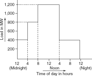
FIG. 1.1 Daily load curve
An annual load curve is a plot of the load demand of the consumer against time in hours of the year (1 year = 8,760 hours).
Significance: From the daily load curve shown in Fig. 1.1, the following information can be obtained:
- Observe the variation of load on the power system during different hours of the day.
- Area under this curve gives the number of units generated in a day.
- Highest point on that curve indicates the maximum demand on the power station on that day.
- The area of this curve divided by 24 hours gives the average load on the power station in the day.
- It helps in selection of the rating and number of generating units required.
1.3 LOAD–DURATION CURVE
The load–duration curve is a plot of the load demands (in units of power) arranged in a descending order of magnitude (on the y-axis) and the time in hours (on the x-axis). The load–duration curve can be drawn as shown in Fig. 1.2.
FIG. 1.2 Load–duration curve
1.4 INTEGRATED LOAD–DURATION CURVE
The integrated load–duration curve is a plot of the cumulative number of units of electrical energy (on the x-axis) and the load demand (on the y-axis).
In the operation of hydro- electric plants, it is necessary to know the amount of energy between different load levels. This information can be obtained from the load–duration curve. Thus, let the duration curve of a particular power station be as indicated in Fig. 1.3(a); obviously the area enclosed by the load–duration curve represents the daily energy generated (in MWh).
The minimum load on the station is d1 (MW). The energy generated during the 24-hour period is 24 d1 (MWh), i.e., the area of the rectangle od1b1a1. So, we can assume that the energy generated varies linearly with the load demand from zero to d1 to d2 MW as indicated in Fig. 1.3(a). As the load demand increases from d1 to d2 MW, the total energy generated will be less than 24 d2 MWh, since the load demand of d2 MW persists for a duration of less than 24 hours. The total energy generated is given by the area od2 b2 a1. So, the energy generated between the load demands of d2 and d1 is (area od2b2a1 – area od1b1a1) = area d1d2b1 (shown cross-latched in Fig. 1.3(a)).
Now, if the total number of units generated was to be plotted as abscissa corresponding to a given load, we shall obtain what is called the integrated load–duration curve. Thus, if the area od2b2a1 were designated as c2 (MWh), then point p has the co-ordinates (e2, d2) on the integrated load–duration curve shown in Fig. 1.3(b).
The integrated load–duration curve is also the plot of the cumulative integration of area under the load curve starting at zero loads to the particular load. It exhibits an increasing slope upto the peak load.
1.4.1 Uses of integrated load–duration curve
- The amount of energy generated between different load levels can be obtained.
- From acknowledgment of the daily energy requirements, the load that can be carried on the base or peak can be easily determined.
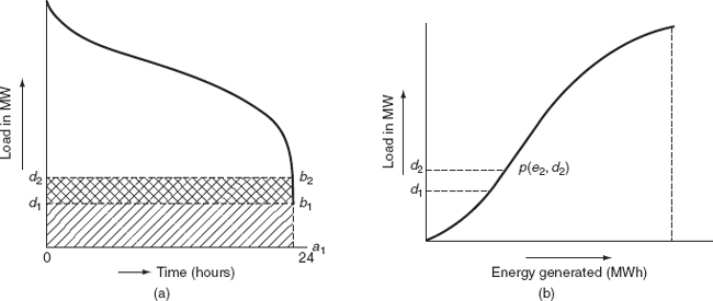
FIG. 1.3 Integrated load–duration curve
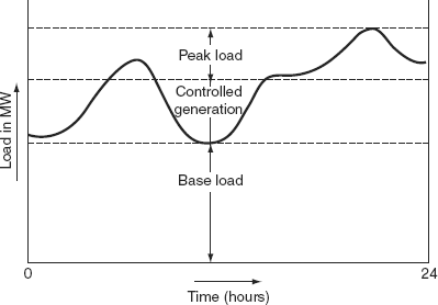
FIG. 1.4 Daily load curve
To have a clear idea of ‘base-load’ and ‘peak load’, let us consider a power system, the daily load curve of which is depicted in Fig. 1.4.
In a power system, there may be several types of generating stations such as hydro-electric stations, fossil-fuel-fired stations, nuclear stations, and gas-turbine-driven generating stations. Of these stations, some act as base-load stations, while others act as peak load stations.
Base-load stations run at 100% capacity on a 24-hour basis. Nuclear reactors are ideally suited for this purpose.
Intermediate or controlled-power generation stations normally are not fully loaded. Hydro-electric stations are the best choice for this purpose.
Peak load stations operate during the peak load hours only. Since the gas-turbine-driven generators can pick up the load very quickly, they are best suited to serve as peak load stations. Where available, pumped-storage hydro-electric plants can be operated as peak load stations.
A base-load station operates at a high-load factor, whereas the peak load plant operates at a low-load factor. So, the base-load station should have low operating costs.
1.5 DEFINITION OF TERMS AND FACTORS
Several terms are used in connection with power supply to an area, whether it be for the first time (as is the case when the area is being electrified for the first time) or subsequently (due to the load growth). These terms are explained below.
1.5.1 Connected load
A consumer, for example, a domestic consumer, may have several appliances rated at different wattages. The sum of these ratings is his/her connected load.
Connected load is the sum of the ratings (W, kW, or MW) of the apparatus installed on a consumer’s premises.
1.5.2 Maximum demand
It is the maximum load used by a consumer at any time. It can be less than or equal to the connected load. If all the devices connected in the consumer’s house run to their fullest extent simultaneously, then the maximum demand will be equal to the connected load. But generally, the actual maximum demand will be less than the connected load since all the appliances are never used at full load at a time.
The maximum demand is usually measured in units of kilowatts (kW) or megawatts (MW) by a maximum demand indicator. (Usually, in the case of high-tension consumers, the maximum demand is measured in terms of kVA or MVA.)
1.5.3 Demand factor
The ratio of the maximum demand to the connected load is called the ‘demand factor’:
Note: Maximum demand and the connected load are to be expressed in the same units (W, kW, or MW).
1.5.4 Average load
If the number of kWh supplied by a station in one day is divided by 24 hours, then the value obtained is known as the daily average load:
Daily average load ![]()
Monthly average load ![]()
Yearly average load ![]()
1.5.5 Load factor
The ratio of the average demand to the maximum demand is called the load factor:
Load factor (LF) ![]()
If the plant is in operation for a period T,
Load factor

The load factor may be a daily load factor, a monthly load factor, or an annual load factor, if the time period is considered in a day or a month or a year, respectively. Load factor is always less than one because average load is smaller than the maximum demand. It plays a key role in determining the overall cost per unit generated. Higher the load factor of the power station, lesser will be the cost per unit generated.
1.5.6 Diversity factor
Diversity factor is the ratio of the sum of the maximum demands of a group of consumers to the simultaneous maximum demand of the group of consumers:
Diversity factor ![]()
A power system supplies load to various types of consumers whose maximum demands generally do not occur at the same time. Therefore, the maximum demand on the power system is always less than the sum of individual maximum demands of the consumers.
A high diversity factor implied that with a smaller maximum demand on the station, it is possible to cater to the needs of several consumers with varying maximum demands occurring at different hours of the day. The lesser the maximum demand, the lesser will be the capital investment on the generators. This helps in reducing the overall cost of the units (kWh) generated.
Thus, a higher diversity factor and a higher load factor are the desirable characteristics of the load on a power station. The load factor can be improved by encouraging the consumers to use power during off-peak hours with certain incentives like offering a reduction in the cost of energy consumed during off-peak hours.
1.5.7 Plant capacity
It is the capacity or power for which a plant or station is designed. It should be slightly more than the maximum demand. It is equal to the sum of the ratings of all the generators in a power station:
1.5.8 Plant capacity factor
It is the ratio of the average demand on the station to the maximum installed capacity of the station.
Plant capacity factor ![]()
1.5.9 Utilization factor (or plant-use factor)
It is the ratio of kWh generated to the product of the plant capacity and the number of hours for which the plant was in operation:
Plant-use factor ![]()
1.5.10 Firm power
It is the power that should always be available even under emergency.
1.5.11 Prime power
It is the maximum power (may be thermal or hydraulic or mechanical) continuously available for conversion into electric power.
1.5.12 Dump power
This is the term usually used in hydro-electric plants and it represents the power in excess of the load requirements. It is made available by surplus water.
1.5.13 Spill power
It is the power that is produced during floods in a hydro-power station.
1.5.14 Cold reserve
It is the reserve-generating capacity that is not in operation, but can be made available for service.
1.5.15 Hot reserve
It is the reserve-generating capacity that is in operation, but not in service.
1.5.16 Spinning reserve
It is the reserve-generating capacity that is connected to bus bars and is ready to take the load.
1.6 BASE LOAD AND PEAK LOAD ON A POWER STATION
Base load: It is the unvarying load that occurs almost during the whole day on the station.
Peak load: It is the various peak demands of load over and above the base load of the station.
Example 1.1: A generating station has a maximum demand of 35 MW and has a connected load of 60 MW. The annual generation of units is 24 × 107 kWh. Calculate the load factor and the demand factor.
Solution:
No. of units generated annually |
= |
24 × 107 kWh |
No. of hours in a year (assuming 365 days in a year) |
= |
365 × 24 |
|
= |
8,760 hours |
∴ Average load on the station
∴ Load Factor
Demand factor
Example 1.2: A generating station supplies four feeders with the maximum demands (in MW) of 16, 10, 12, and 7 MW. The overall maximum demand on the station is 20 MW and the annual load factor is 45%. Calculate the diversity factor and the number of units generated annually.
Solution:
Sum of maximum demands = 16 + 10 + 12 + 7 = 45 MW
Simultaneous maximum demand = 20 MW
∴ Diversity factor
Average demand = (maximum demand) × (load factor)
= 20 × 0.45 = 9 MW
∴ No. of units generated annually = 9 × 8,760 = 78,840 MWh
Alternatively,
Annual load factor ![]()
i.e,
so that the number of units generated annually = 0.45 × 20 × 8,760 MWh
= 78,840 MWh
Example 1.3: The yearly load–duration curve of a power plant is a straight line (Fig. 1.5). The maximum load is 30 MW and the minimum load is 20 MW. The capacity of the plant is 35MW. Calculate the plant capacity factor, the load factor, and the utilization factor.
Solution:
No. of units generated per year = Area OACD = Area OBCD + Area BAC
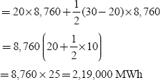
∴ Average annual load
∴ Load factor ![]()
Plant capacity factor ![]()
Utilization factor ![]()
Alternatively,
Utilization factor ![]()

FIG. 1.5 Load–duration curve
Example 1.4: Calculate the total annual energy generated, if the maximum demand on a power station is 120 MW and the annual load factor is 50%.
Solution:
Maximum demand on a power station = 120 MW
Annual load factor = 50%
Load factor ![]()
∴ Energy generated/annum |
= |
maximum demand × LF × hours in a year |
|
= |
(120 × 103) × (0.5) × (24 × 365) kWh |
|
= |
525.6 × 10⁶ kWh |
Example 1.5: Determine the demand factor and the load factor of a generating station, which has a connected load of 50 MW and a maximum demand of 25 MW, the units generated being 40 × 106/annum.
Solution:
Connected load |
= |
50 MW |
Maximum demand |
= |
25 MW |
Units generated |
= |
40 × 106/annum |
Demand factor ![]()
Average demand
Load factor ![]()
Example 1.6: Calculate the annual load factor of a 120 MW power station, which delivers 110 MW for 4 hours, 60 MW for 10 hours, and is shut down for the rest of each day. For general maintenance, it is shut down for 60 days per annum.
Solution:
Capacity of power station |
= |
120 MW |
Power delivered |
= |
110 MW for 4 hours |
|
= |
60 MW for 10 hours |
|
= |
0 for the rest of each day |
And for general maintenance, it is shut down for 60 days per annum.
Energy supplied in 1 day = (110 × 4) + (60 × 10) = 1,040 MWh
No. of working days in a year = 365 − 60 = 305
Energy supplied per year = 1,040 × 305 = 3,17,200 MWh
Annual load factor
Example 1.7: customer-connected loads are 10 lamps of 60 W each and two heaters of 1,500 W each. His/her maximum demand is 2 kW. On average, he/she uses 10 lamps, 7 hours a day, and each heater for 5 hours a day. Determine his/her: (i) average load, (ii) monthly energy consumption, and (iii) load factor.
Solution:
Maximum demand = 2 kW
Connected load = 10 × 60 + 2 × 1,500 = 3,600 W
Daily energy consumption = number of lamps used × wattage of each lamp × working hours per day + number of heaters × wattage of each heater × working hours per day
|
= |
10 × 60 × 7 + 2 × 1,500 × 5 |
|
= |
19.2 kWh |
- Average load

-
Monthly energy consumption
=
daily energy consumption × no. of days in a month
=
19.2 × 30 = 576 kWh
=
576 kWh
- Monthly load factor

Example 1.8: The maximum demand on a generating station is 20 MW, a load factor of 75%, a plant capacity factor of 50%, and a plant-use factor of 80%. Calculate the following:
- daily energy generated,
- reserve capacity of the plant,
- maximum energy that could be produced daily if the plant were in use all the time.
Solution:
Maximum demand, MD |
= |
20 MW |
Load factor, LF |
= |
75% |
Power capacity factor |
= |
50% |
Plant-use factor |
= |
80% |
Average load |
= |
MD × LF |
|
= |
20 × 0.75 = 15 MW |
- Daily energy generated = average load × 24 = 15 × 24 = 360 MWh
- Power station installed capacity =

Plant reserve capacity = installed capacity − maximum demand
= 30 − 20
= 10 MW
- The maximum energy that can be produced daily if the plant is running all the time
Example 1.9: A certain power station’s annual load–duration curve is a straight line from 25 to 5 MW (Fig. 1.6). To meet this load, three turbine-generator units, two rated at 15 MW each and one rated at 7.5 MW are installed. Calculate the following:
- installed capacity;
- plant factor;
- units generated per annum;
- utilization factor.
Solution:
- Installed capacity = 2 × 15 + 7.5
= 37.5 MW
- From the load–duration curve shown in Fig. 1.6,
Average demand

∴ Plant factor

- Units generated per annum = area (in kWh) under load–duration curve
- Utilization factor

FIG. 1.6 Load–duration curve
Example 1.10: A consumer has a connected load of 12 lamps each of 100 W at his/ her premises. His/ her load demand is as follows:
From midnight to 5 A.M.: 200 W.
5 A.M. to 6 P.M.: no load.
6 P.M. to 7 P.M.: 700 W.
7 P.M. to 9 P.M.: 1,000 W.
9 P.M. to midnight: 500 W.
Draw the load curve and calculate the (i) energy consumption during 24 hours, (ii) demand factor, (iii) average load, (iv) maximum demand, and (v) load factor.
Solution:
From Fig. 1.7,
- Electrical energy consumption during the day = area of load curve
= 200 × 5 + 700 × 1 + 1,000 × 2 + 500 × 3
= 5,200 Wh
= 5.2 kWh
- Average load

- Demand factor

- Maximum demand = 1,000 W
- Load factor

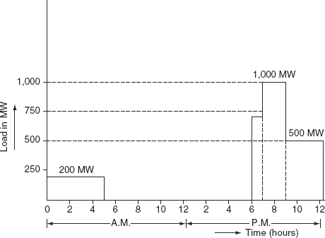
FIG. 1.7 Load curve
Example 1.11: Calculate the diversity factor and the annual load factor of a generating station, which supplies loads to various consumers as follows:
Industrial consumer = 2,000 kW;
Commercial establishment = 1,000 kW
Domestic power = 200 kW;
Domestic light = 500 kW
and assume that the maximum demand on the station is 3,000 kW, and the number of units produced per year is 50×105.
Solution:
Load industrial consumer |
= 2,000 kW |
Load commercial establishment |
= 1,000 kW |
Domestic power load |
= 200 kW |
Domestic lighting load |
= 500 kW |
Maximum demand on the station |
= 3,000 kW |
Number of kWh generated per year |
= 50 × 105 |
Diversity factor ![]()
Average demand

Load factor ![]()
Example 1.12: Calculate the reserve capacity of a generating station, which has a maximum demand of 20,000 kW, the annual load factor is 65%, and the capacity factor is 45%.
Solution:
Maximum demand |
= |
20,000 kW |
Annual load factor |
= |
65% |
Capacity factor |
= |
45% |
Energy generated/annum |
= |
maximum demand LF hours in a year |
|
= |
(20,000) × (0.65) × (8,760) kWh = 113.88 × 10⁶ kWh |
|
|
|
|
|
|
Reserve capacity |
= |
plant capacity − maximum demand |
|
= |
28,888.89 − 20,000 = 8,888.89 kW |
Example 1.13: The maximum demand on a power station is 600 MW, the annual load factor is 60%, and the capacity factor is 45%. Find the reserve capacity of the plant.
Solution:
Utilization factor ![]()
Plant capacity ![]()
Reserve capacity |
= |
plant capacity − maximum demand |
|
= |
800 − 600 |
|
= |
200 MW |
Example 1.14: A power station’s maximum demand is 50 MW, the capacity factor is 0.6, and the utilization factor is 0.85. Calculate the following: (i) reserve capacity and (ii) annual energy produced.
Solution:
Energy generated/annum = maximum demand × load factor × hours in a year
= (50 × LF × 8,760) MWh
Load factor ![]()
Energy generated/annum |
= |
50 × 0.706 × 8,760 |
|
= |
3,09,228 MWh = 0.3 × 10⁶ MWh |
Plant capacity ![]()
Reserve capacity |
= |
plant capacity − maximum demand |
|
= |
58.82 − 50 |
|
= |
8.82 MW |
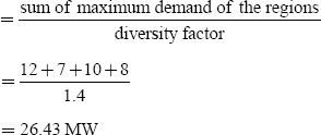
Example 1.15: A power station is to feed four regions of load whose peak loads are 12, 7, 10, and 8 MW. The diversity factor at the station is 1.4 and the average annual load factor is 65%. Determine the following: (i) maximum demand on the station, (ii) annual energy supplied by the station, and (iii) suggest the installed capacity.
Solution:
- Maximum demand on station
- Units generated/annum = max. demand × LF × house in a year
= (26.43 × 103) × 0.65 × 8,760 kWh
= 150.49 × 10⁶ kMh
- The installed capacity of the station should be 15% to 20% more than the maximum demand in order to meet the future growth of load.
Taking the installed capacity to be 20% more than the maximum demand,
Installed capacity = 1.2 × max. demand
= 1.2 × 26.43
= 31.716 ≅ 32 MW
1.7 LOAD FORECASTING
Electrical energy cannot be stored. It has to be generated whenever there is a demand for it. It is, therefore, imperative for the electric power utilities that the load on their systems should be estimated in advance. This estimation of load in advance is commonly known as load forecasting. It is necessary for power system planning.
Power system expansion planning starts with a forecast of anticipated future load requirements. The estimation of both demand and energy requirements is crucial to an effective system planning. Demand predictions are used for determining the generation capacity, transmission, and distribution system additions, etc. Load forecasts are also used to establish procurement policies for construction capital energy forecasts, which are needed to determine future fuel requirements. Thus, a good forecast, reflecting the present and future trends, is the key to all planning.
In general, the term forecast refers to projected load requirements determined using a systematic process of defining future loads in sufficient quantitative detail to permit important system expansion decisions to be made. Unfortunately, the consumer load is essentially uncontrollable although minor variations can be affected by frequency control and more drastically by load shedding. The variation in load does exhibit certain daily and yearly pattern repetitions, and an analysis of these forms the basis of several load-prediction techniques.
1.7.1 Purpose of load forecasting
- For proper planning of power system;
- For proper planning of transmission and distribution facilities;
- For proper power system operation;
- For proper financing;
- For proper manpower development;
- For proper grid formation;
- For proper electrical sales.
(i) For Proper Planning of Power System
- To determine the potential need for additional new generating facilities;
- To determine the location of units;
- To determine the size of plants;
- To determine the year in which they are required;
- To determine that they should provide primary peaking capacity or energy or both;
- To determine whether they should be constructed and owned by the Central Government or State Government or Electricity Boards or by some other autonomous corporations.
(ii) For Proper Planning of Transmission and Distribution Facilities
For planning the transmission and distribution facilities, the load forecasting is needed so that the right amount of power is available at the right place and at the right time. Wastage due to misplanning like purchase of equipment, which is not immediately required, can be avoided.
(iii) For Proper Power System Operation
Load forecast based on correct values of demand and diversity factor will prevent overdesigning of conductor size, etc. as well as overloading of distribution transformers and feeders. Thus, they help to correct voltage, power factor, etc. and to reduce the losses in the distribution system.
(iv) For Proper Financing
The load forecasts help the Boards to estimate the future expenditure, earnings, and returns and to schedule its financing program accordingly.
(v) For Proper Manpower Development
Accurate load forecasting annually reviewed will come to the aid of the Boards in their personnel and technical manpower planning on a long-term basis. Such a realistic forecast will reduce unnecessary expenditure and put the Boards’ finances on a sound and profitable footing.
(vi) For Proper Grid Formation
Interconnections between various state grids are now becoming more and more common and the aim is to have fully interconnected regional grids and ultimately even a super grid for the whole country. These expensive high-voltage interconnections must be based on reliable load data, otherwise the generators connected to the grid may frequently fall out of step causing power to be shut down.
(vii) For Proper Electrical Sales
In countries, where spinning reserves are more, proper planning and the execution of electrical sales program are aided by proper load forecasting.
1.7.2 Classification of load forecasting
The load forecasting can be classified as: (i) demand forecast and (ii) energy forecast.
(i) Demand Forecast
This is used to determine the capacity of the generation, transmission, and distribution system additions. Future demand can be predicted on the basis of fast rate of growth of demand from past history and government policy. This will give the expected rate of growth of load.
(ii) Energy Forecast
This is used to determine the type of facilities required, i.e., future fuel requirements.
1.7.3 Forecasting procedure
Depending on the time period of interest, a specific forecasting procedure may be classified as:
- Short-term.
- Medium (intermediate)-term.
- Long-term technique.
(1) Short-Term Forecast
For day-to-day operation, covering one day or a week, short-term forecasting is needed in order to commit enough generating capacity formatting the forecasting demand and for maintaining the required spinning reserve. Hence, it is usually done 24 hours ahead when the weather forecast for the following day becomes available from the meteorological office. This mostly consists of estimating the weather-dependent component and that due to any special event or festival because the base load for the day is already known.
The power supply authorities can build up a weather load model of the system for this purpose or can consult some tables. The final estimate is obviously done after accounting the transmission and distribution losses of the system. In addition to the prediction of hourly values, a short-term load forecasting (STLF) is also concerned with forecasting of daily peak-system load, system load at certain times of a day, hourly values of system energy, and daily and weekly system energy.
Applications of STLF are mainly:
- To drive the scheduling functions that decide the most economic commitment of generation sources.
- To access the power system security based on the information available to the dispatchers to prepare the necessary corrective actions.
- To provide the system dispatcher with the latest weather predictions so that the system can be operated both economically and reliably.
(2) Long-Term Forecast
This is done for 1–5 years in advance in order to prepare maintenance schedules of the generating units, planning future expansion of the generating capacity, enter into an agreement for energy interchange with the neighboring utilities, etc. Basically, two approaches are available for this purpose and are discussed as follows.
(a) Peak Load Approach
In this case, the simplest approach is to extrapolate the trend curve, which is obtained by plotting the past values of annual peaks against years of operation. The following analytical functions can be used to determine the trend curve.
- Straight line, Y = a + bx
- Parabola, Y = a + bx + cx2
- S-curve, Y = a + bx + cx2 + dx3
- Exponential, Y = ce dx
- Gompertz, logeY = a + ce dx
In the above, Y represents peak loads and x represents time in years. The most common method of finding coefficients a, b, c, and d is the least squares curve-fitting technique.
The effect of weather conditions can be ignored on the basis that weather conditions, as in the past, are to be expected during the period under consideration but the effect of the change in the economic condition should be accommodated by including an economic variable when extrapolating the trend curve. The economic variable may be the predicted national income, gross domestic product, etc.
(b) Energy Approach
Another method is to forecast annual energy sales to different classes of customers like residential, commercial, industrial, etc., which can then be converted to annual peak demand using the annual load factor. A detailed estimation of factors such as rate of house building, sale of electrical appliances, growth in industrial and commercial activities are required in this method. Forecasting the annual load factor also contributes critically to the success of the method. Both these methods, however, have been used by the utilities in estimating their long-term system load.
KEY NOTES
- A load curve is a plot of the load demand (on the y-axis) versus the time (on the x-axis) in the chronological order.
- The load–duration curve is a plot of the load demands (in units of power) arranged in a descending order of magnitude (on the y-axis) and the time in hours (on the x-axis).
- In the operation of hydro-electric plants, it is necessary to know the amount of energy between different load levels. This information can be obtained from the load–duration curve.
- The integrated load–duration curve is also the plot of the cumulative integration of area under the load curve starting at zero loads to the particular load.
- A base-load station operates at a high-load factor while the peak load plant operates at a-low load factor.
- Demand factor is the ratio of the maximum demand to the connected load.
- Load factor is the ratio of the average demand to the maximum demand. Higher the load factor of the power station, lesser will be the cost per unit generated.
- Diversity factor is the ratio of the sum of the maximum demands of a group of consumers and the simultaneous maximum demand of the group of consumers.
- Base load is the unvarying load that occurs almost the whole day on the station.
- Peak load is the various peak demands of load over and above the base load of the station.
SHORT QUESTIONS AND ANSWERS
- What is meant by connected load?
It is the sum of the ratings of the apparatus installed on a consumer’s premises.
- Define the maximum demand.
It is the maximum load used by a consumer at any time.
- Define the demand factor.
The ratio of the maximum demand to the connected load is called the demand factor.
- Define the average load.
If the number of kWh supplied be a station in one day is divided by 24 hours, then the value obtained is known as the daily average load.
- Define the load factor.
It is the ratio of the average demand to the maximum demand.
- Define the diversity factor.
It is the ratio of the sum of the maximum demands of a group of consumers to the simultaneous maximum demand of the group of consumers.
- Define the plant capacity.
It is the capacity or power for which a plant or station is designed.
- Define the utilization factor.
It is the ratio of kWh generated to the product of the plant capacity and the number of hours for which the plant was in operation.
- What is meant by base load?
It is the unvarying load that occurs almost the whole day on the station.
- What is meant by peak load?
It is the various peak demands of load over and above the base load of the station.
- What is meant by load curve?
A load curve is a plot of the load demand versus the time in the chronological order.
- What is meant by load–duration curve?
The load–duration curve is a plot of the load demands arranged in a descending order of magnitude versus the time in hours.
MULTIPLE-CHOICE QUESTIONS
- In order to have a low cost of electrical generation,
- The load factor and diversity factor are high.
- The load factor should be low but the diversity factor should be high.
- The load factor should be high but the diversity factor should be low.
- The load factor and the diversity factor should be low.
- A power plant having maximum demand more than the installed capacity will have utilization factor:
- Less than 100%.
- Equal to 100%.
- More than 100%.
- None of these.
- The choice of number and size of units in a station are governed by best compromise between:
- A plant load factor and capacity factor.
- Plant capacity factor and plant-use factor.
- Plant load factor and use factor.
- None of these.
- If a plant has zero reserve capacity, the plant load factor always:
- Equals plant capacity factor.
- Is greater than plant capacity factor.
- Is less than plant capacity factor.
- None of these.
- If some reserve is available in a power plant,
- Its use factor is always greater than its capacity factor.
- Its use factor equals the capacity factor.
- Its use factor is always less than its capacity factor.
- None of these.
- A higher load factor means:
- Cost per unit is less.
- Less variation in load.
- The number of units generated are more.
- All of these.
- The maximum demand of two power stations is the same. If the daily load factors of the stations are 10 and 20%, then the units generated by them are in the ratio:
- 2:1.
- 1:2.
- 3:3.
- 1:4.
- A plant had an average load of 20 MW when the load factor is 50%. Its diversity factor is 20%. The sum of max. demands of all loads amounts to:
- 12 MW.
- 8 MW.
- 6 MW.
- 4 MW.
- A peak load station:
- Should have a low operating cost.
- Should have a low capital cost.
- Can have a operating cost high.
- (a)and (c).
- (b)and(c).
- Two areas A and B have equal connected loads; however the load diversity in area A is more than in B, then:
- Maximum demand of two areas is small.
- Maximum demand of A is greater than the maximum demand of B.
- The maximum demand of B is greater than the maximum demand of A.
- The maximum demand of A more or less than that of B.
- The area under the daily load curve gives
- The number of units generated in the day.
- The average load of the day.
- The load factor of the day.
- The number of units generated in the year.
- The annual peak load on a 60-MW power station is 50 MW. The power station supplies loads having average demands of 9, 10, 17, and 20 MW. The annual load factor is 60%. The average load on the plant is:
- 4,000 kW.
- 30,000 kW.
- 2,000 kW.
- 1,000 kW.
- A generating station has a connected load of 40 MW and a maximum demand of 20 MW. The demand factor is:
- 0.7.
- 0.6.
- 0.59.
- 0.4.
- A 100 MW power plant has a load factor of 0.5 and a utilization factor of 0.2. Its average demand is:
- 10 MW.
- 5 MW.
- 7 MW.
- 6 MW.
- The value of the demand factor is always:
- Less than one.
- Equal to one.
- Greater than one.
- None of these.
- If capacity factor = load factor, then:
- Utilization factor is zero.
- Utilization capacity is non-zero.
- Utilization factor is equal to one.
- None of these.
- If capacity factor = load factor, then the plant’s
- Reserve capacity is maximum.
- Reserve capacity is zero.
- Reserves capacity is less.
- None of these.
- Installed capacity of power plant is:
- More than the maximum demand.
- Less than the maximum demand.
- Equal to the maximum demand.
- Both and.
- In an interconnected system, diversity factor determining:
- Decreases.
- Increases.
- Zero.
- None of these.
- The knowledge of diversity factor helps in determining:
- Plant capacity.
- Reserve capacity.
- Maximum demand.
- Average demand.
- A power station has an installed capacity of 300 MW. Its capacity factor is 50% and its load factor is 75%. Its maximum demand is:
- 100 MW.
- 150 MW.
- 200 MW.
- 250 MW.
- The connected load of a consumer is 2 kW and his/her maximum demand is 1.5 kW. The load factor of the consumer is:
- 0.75.
- 0.375.
- 1.33.
- none of these.
- The maximum demand of a consumer is 2 kW and his/her daily energy consumption is 20 units. His/her load factor is:
- 10.15%.
- 41.6%.
- 50%.
- 52.6%.
- In a power plant, a reserve-generating capacity, which is not in service but in operation is known as:
- Hot reserve.
- Spinning reserve.
- Cold reserve.
- Firm power.
- The power intended to be always available is known as:
- Hot reserve.
- Spinning reserve.
- Cold reserve.
- Firm power.
- In a power plant, a reserve-generating capacity, which is in service but not in operation is:
- Hot reserve.
- Spinning reserve.
- Cold reserve.
- Firm power.
- Which of the following is a correct factor?
- Load factor = capacity × utilization factor.
- Utilization factor = capacity factor × load factor.
- Utilization factor = load factor/utilization factor.
- Capacity factor = load factor × utilization factor.
- If the rated plant capacity and maximum load of generating station are equal, then:
- Load factor is 1.
- Capacity factor is 1.
- Load factor and capacity factor are equal.
- Utilization factor is poor.
- The capital cost of plant depends on:
- Total installed capacity only.
- Total number of units only.
- Both and.
- None of these.
- The reserve capacity in a system is generally equal to:
- Capacity of the largest generating unit.
- Capacity of two largest generating units.
- The total generating capacity.
- None of the above.
- The maximum demand of a consumer is 5 kW and his/her daily energy consumption is 24 units. His/her % load factor is:
- 5.
- 20.
- 24.
- 48.
- If load factor is poor, then:
- Electric energy produced is small.
- Charge per kWh is high.
- Fixed charges per kWh is high.
- All of the above.
- If a generating station had maximum loads for a day at 100 kW and a load factor of 0.2, its generation in that day was:
- 8.64 MWh.
- 21.6 units.
- 21.6 units.
- 2,160 kWh.
- The knowledge of maximum demand is important as it helps in determining:
- Installed capacity of the plant.
- Connected load of the plant.
- Average demand of the plant.
- Either (a) or(b).
- A power station is connected to 4.5 and 6 kW. Its daily load factor was calculated as 0.2, where its generation on that day was 24 units. Calculate the demand factor.
- 2.6.
- 3.1.
- 3.0.
- 0.476.
- A 50-MW power station had produced 24 units in a day when its maximum demand was 50 Mw. Its plant load factor and capacity factor that day in % were:
- 1 and 2.
- 2 and 3.
- 2 and 2.
- 4 and 3.
- Load curve of a power generation station is always:
- Negative.
- Zero slope.
- Positive.
- Any combination of (a), (b), and (c).
- Load curve helps in deciding the:
- Total installed capacity of the plant.
- Size of the generating units.
- Operating schedule of the generating units.
- All of the above.
- The load factor for domestic loads may be taken:
- About 85%.
- 50−60%.
- 25−50%.
- 20−15%.
REVIEW QUESTIONS
- Explain the significance of the daily load curve.
- Discuss the difference between the load curve and the load–duration curve.
- Explain the differences in operations of peak load and base-load stations.
- Explain the significance of the load factor and the diversity factor.
- Define the following:
- Load factor,
- Demand factor,
- Diversity factor,
- Plant capacity factor, and
- Utilization factor.
- Explain the load forecasting procedures.
PROBLEMS
- Calculate diversity factor and annual load factor of a generating station that supplies loads to various consumers as follows:
Industrial consumer = 1,500 kW;
Commercial establishment = 7,500 kW
Domestic power = 100 kW;
Domestic light = 400 kW
In addition, assume that the maximum demand on the station is 2,500 kW and the number of units produced per year is 40 × 105kWh.
- A power station is to feed four regions of load whose peak loads are 10, 5, 14, and 6 MW, respectively. The diversity factor at the station is 1.3 and the average annual load factor is 60%. Determine the following: (i) maximum demand on the station, (ii) annual energy supplied by the station, and (iii) suggest the installed capacity.
- A certain power station’s annual load–duration curve is a straight line from 20 to 7 MW. To meet this load, three turbine-generator units, two rated at 12 MW each and one rated at 8 MW are installed. Calculate the following:
- Installed capacity,
- Plant factor,
- Units generated per annum,
- Utilization factor.