
7
Load Frequency Control-I
OBJECTIVES
After reading this chapter, you should be able to be able to:
- study the governing characteristics of a generator
- study the load frequency control (LFC)
- develop the mathematical models for different components of a power system
- observe the steady state and dynamic analysis of a single-area power system with and without integral control
7.1 INTRODUCTION
In a power system, both active and reactive power demands are never steady and they continually change with the rising or falling trend. Steam input to turbo-generators or water input to hydro-generators must, therefore, be continuously regulated to match the active power demand, failing which the machine speed will vary with consequent change in frequency and it may be highly undesirable. The maximum permissible change in frequency is ±2%. Also, the excitation of the generators must be continuously regulated to match the reactive power demand with reactive power generation; otherwise, the voltages at various system buses may go beyond the prescribed limits. In modern large interconnected systems, manual regulation is not feasible and therefore automatic generation and voltage regulation equipment is installed on each generator. The controllers are set for a particular operating condition and they take care of small changes in load demand without exceeding the limits of frequency and voltage. As the change in load demand becomes large, the controllers must be reset either manually or automatically.
7.2 NECESSITY OF MAINTAINING FREQUENCY CONSTANT
Constant frequency is to be maintained for the following functions:
- All the AC motors should require constant frequency supply so as to maintain speed constant.
- In continuous process industry, it affects the operation of the process itself.
- For synchronous operation of various units in the power system network, it is necessary to maintain frequency constant.
- Frequency affects the amount of power transmitted through interconnecting lines.
- Electrical clocks will lose or gain time if they are driven by synchronous motors, and the accuracy of the clocks depends on frequency and also the integral of this frequency error is loss or gain of time by electric clocks.
7.3 LOAD FREQUENCY CONTROL
Load frequency control (LFC) is the basic control mechanism in the power system operation. Whenever there is a variation in load demand on a generating unit, there is momentarily an occurrence of unbalance between real-power input and output. This difference is being supplied by the stored energy of the rotating parts of the unit.
The kinetic energy of any unit is given by
where I is the moment of inertia of the rotating part and ω the angular speed of the rotating part.
If KE reduces, ω decreases; then the speed falls, hence the frequency reduces. The change in frequency Δf is sensed and through a speed-governor system, it is fed back to control the position of the inlet valve of the prime mover, which is connected to the generating unit. It changes the input to the prime mover suitably and tries to bring back the balance between the real-power input and output. Hence, it can be stated that the frequency variation is dependent on the real-power balance of the system.
The LFC also controls the real-power transfer through the interconnecting transmission lines by sensing the change in power flow through the tie lines.
7.4 GOVERNOR CHARACTERISTICS OF A SINGLE GENERATOR
Prime movers driving the generators are fitted with governors, which are regarded as primary control elements in the LFC system. Governors sense the change in a speed control mechanism to adjust the opening of steam valves in the case of steam turbines and the opening of water gates in the case of water turbines. The characteristics of a typical governor of a steam turbine are shown in Fig. 7.1, which is linearized by dotted lines for studying the system behavior.
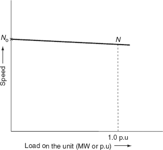
FIG. 7.1 Characteristics of a typical governor of a steam turbine
The amount of speed drop as the load on the turbine is increased from no load to its full-load value is (No–N), where No is the speed at no load and N is the speed at rated load.
The steady-state speed regulation in per unit is given by
The value of R varies from 2% to 6% for any generating unit. Since the frequency and speed are directly related, the speed regulation can also be expressed as the ratio of the change in frequency from no load to its full load to the rated frequency of the unit:
i.e., ![]()
If there is a 4% speed regulation of a unit, then for a rated frequency of 50 Hz, there will be a drop of 2 Hz in frequency.
If the generation is increased by ΔPG due to a static frequency drop of Δf, then the speed regulation can be defined as the ratio of the change in frequency to the corresponding change in real-power generation:
i.e., ![]()
The unit of R is taken as Hz per MW. In practice, power is measured in per unit and hence R is in Hz/p.u. MW.
In Fig. 7.2, the turbine is operating with 99% of no-load speed at 25% of full-load power and if the load is increased to 50%, the speed drops to 98%. Let ‘A’ be the initial operating point of the turbine at 50% load and if the load is dropped to 25%, the speed increases to 99%. In order to keep the speed at 25% of the load same as at ‘A’, the governor setting has to be changed by changing the spring tension in the fly-ball type of governor. This will result in speed characteristics indicated by the dotted line parallel to the first one and below it, passing through the point A′, which is the point of intersection of the new speed line and 25% load line. Hence, the turbine can be adjusted to carry any given load at any desired speed.

FIG. 7.2 Speed-governor setting
This type of shifting the speed or frequency characteristic parallel to itself is known as supplementary control. It is adopted in on-line control to ensure proper load division among the running units and to maintain the system frequency. There is another method of changing the slope of the governor characteristics. This is achieved by changing the ratio of the lever L (refer the speed control mechanism) of the governor and thereby adjusting the parameter R to ensure proper co-ordination with the other units of the system. This adjustment can be made during the off-line condition only.
7.5 ADJUSTMENT OF GOVERNOR CHARACTERISTIC OF PARALLEL OPERATING UNITS
When two generators are running in parallel, the governor characteristic of the first unit (Line 1) is shown towards the right, while that of the second unit (Line 2) is shown towards the left of the frequency axis as shown in Fig. 7.3.
The characteristics are obviously different and hence corresponding to the rated frequency fr, the two units carry loads P1 and P2 so that the system load PD = P1 + P2. If the system load is now increased to P′D, the system frequency will drop down to f ′, since the units can only increase their output by decreasing the speed.
To restore the system frequency, the characteristic of one of the units say of Unit 1 needs to be shifted upwards as indicated by the dotted characteristic, so that it can carry the increased load. The share of Unit 1 will be P1′ and that of Unit 2 will be P2 so that the increased total load, PD′ = P1′ + P2.

FIG. 7.3 Sharing of load by two units (parallel) with a speed-governor characteristics setting
7.6 LFC: (P–f CONTROL)
The LFC, also known as generation control or P–f control, deals with the control of loading of the generating units for the system at normal frequency. The load in a power system is never constant and the system frequency remains at its nominal value only when there is a match between the active power generation and the active power demand. During the period of load change, the deviation from the nominal frequency, which may be called frequency error (Δf), is an index of mismatch and can be used to send the appropriate command to change the generation by adjusting the LFC system. It is basically controlling the opening of the inlet valves of the prime movers according to the loading condition of the system. In the case of a multi-area system, the LFC system also maintains the specified power interchanges between the participating areas. In a smaller system, this control is done manually, but in large systems automatic control devices are used in the loop of the LFC system.
The LFC system, however, does not consider the reactive power flow in the system even though the reactive power flow is also affected to some extent during the fluctuating load condition. But since there is no counterpart of the reactive power in the mechanical side of the system, it does not come within the loop of the LFC system.
7.7 Q–V CONTROL
In this control, the terminal voltage of the generator is sensed and converted into proportionate DC signal and then compared to DC reference voltage. The error in between a DC signal and a DC reference voltage, i.e., Δ |Vi| is taken as an input to the Q–V controller. A control output ΔQci is applied to the exciter.
7.8 GENERATOR CONTROLLERS (P–f AND Q–V CONTROLLERS)
The active power P is mainly dependent on the internal angle δ and is independent of the bus voltage magnitude |V|. The bus voltage is dependent on machine excitation and hence on reactive power Q and is independent of the machine angle δ. Change in the machine angle δ is caused by a momentary change in the generator speed and hence the frequency. Therefore, the load frequency and excitation voltage controls are non-interactive for small changes and can be modeled and analyzed independently.
Figure 7.4 gives the schematic diagram of load frequency (P–f) and excitation voltage (Q–V) regulators of a turbo-generator. The objective of the MW frequency or the P–f control mechanism is to exert control of frequency and simultaneously exchange of the real-power flows via interconnecting lines. In this control, a frequency sensor senses the change in frequency and gives the signal Δfi. The P–f controller senses the change in frequency signal (Δ fi) and the increments in tie-line real powers (ΔPtie), which will indirectly provide information about the incremental state error (Δδi). These sensor signals (Δfi and ΔPtie) are amplified, mixed, and transformed into a real-power control signal ΔPci. The valve control mechanism takes ΔPci as the input signal and provides the output signal, which will change the position of the inlet valve of the prime mover. As a result, there will be a change in the prime mover output and hence a change in real-power generation ΔPGi. This entire P–f control can be yielded by automatic load frequency control (ALFC) loop.
The objective of the MVAr-voltage or Q–V control mechanism is to exert control of the voltage state |Vi|. A voltage sensor senses the terminal voltage and converts it into an equivalent proportionate DC voltage. This proportionate DC voltage is compared with a reference voltage Viref by means of a comparator. The output obtained from the comparator is error signal Δ|Vi| and is given as input to Q–V controller, which transforms it to a reactive power signal command ΔQci and is fed to a controllable excitation source. This results in a change in the rotor field current, which in turn modifies the generator terminal voltage. This entire Q–V control can be yielded by an automatic voltage regulator (AVR) loop.

FIG. 7.4 Schematic diagram of P–f controller and Q–V controller
In addition to voltage regulators at generator buses, equipment is used to control voltage magnitude at other selected buses. Tap-changing transformers, switched capacitor banks, and static VAr systems can be automatically regulated for rapid voltage control.
7.9 P–f CONTROL VERSUS Q–V CONTROL
Any static change in the real bus power ΔPi will affect only the bus voltage phase angles (δi) (since P∝δ), but will leave the bus voltage magnitudes almost unaffected.
Static change in the reactive bus power ΔQi affects essentially only the bus voltage magnitudes (since Q ∝ V 2), but leave the bus voltage phase angles almost unchanged.
Static change in reactive bus power at a particular bus affects the magnitude of that bus voltage most strongly, but in less degree the magnitudes of the bus voltages at remote buses.
7.10 DYNAMIC INTERACTION BETWEEN P–f AND Q–V LOOPS
In a static sense, for small deviations, there is a little interaction between P–f and Q–V loops. During dynamic perturbations, we encounter considerable coupling between two control loops for two following reasons:
- As the voltage magnitude fluctuates at a bus, the real load of that bus will likewise change as a result of the voltage load characteristic
 .
. - As the voltage magnitude fluctuates at a bus, the power transmitted over the lines connected to that bus will change. In other words, the change in Q–V loop will affect the generated emf, which also affects the magnitude of real power.
A dynamic perturbation in the Q–V loop will thus affect the real-power balance in the system. In general, the Q–V loop is much faster than the P–f loop due to the mechanical inertial constants in the P–f loop. If it can be assumed that the transients in the Q–V loop are essentially over before the P–f loop reacts, then the coupling between the two loops can be ignored.
7.11 SPEED-GOVERNING SYSTEM
The speed governor is the main primary tool for the LFC, whether the machine is used alone to feed a smaller system or whether it is a part of the most elaborate arrangement. A schematic arrangement of the main features of a speed-governing system of the kind used on steam turbines to control the output of the generator to maintain constant frequency is as shown in Fig. 7.5.

FIG. 7.5 Speed-governor system
Its main parts or components are as follows:
Fly-ball speed governor: It is a purely mechanical, speed-sensitive device coupled directly to and builds directly on the prime movers to adjust the control valve opening via linkage mechanism. It senses a speed deviation or a power change command and converts it into appropriate valve action. Hence, this is treated as the heart of the system, which controls the change in speed (frequency). As the speed increases, the fly balls move outwards and the point B on linkage mechanism moves upwards. The reverse will happen if the speed decreases.
The horizontal rotating shaft on the lower left may be viewed as an extension of the shaft of a turbine-generator set and has a fixed axis as shown in Fig. 7.5. The vertical shaft, above the fly-ball mechanism, also rotates between fixed bearings. Although its axis is fixed, it can move up and down, transferring its vertical motion to the pilot point B.
Hydraulic amplifier: It is nothing but a single-state hydraulic servomotor interposed between the governor and valve. It consists of a pilot valve and the main piston. With this arrangement, hydraulic amplification is obtained by converting the movement of low-power pilot valve into movement of high-power level main piston.
In hydraulic amplification, a large mechanical force is necessary so that the steam valve could be opened or closed against high-pressure inlet steam.
Speed changer: It provides a steady-state power output setting for the turbines. Its upward movement opens the upper pilot valve so that more steam is admitted to the turbine under steady conditions. This gives rise to higher steady-state power output. The reverse will happen if the speed changer moves downward.
Linkage mechanism: These are linked for transforming the fly-balls moment to the turbine valve (steam valve) through a hydraulic amplifier.
ABC is a rigid link pivoted at point B and CDE is another rigid pivoted link at point D. Link DE provides a feedback from the steam valve moment.
The speed-governing system is basically called the primary control loop in the LFC. If the control valve position is indicated by xE, a small upward movement of point E decreases the steam flow by a considerable amount. It is measured in terms of valve power ΔPv. This flow decrement gets translated into decrement in turbine power output ΔPT.
With the help of linkage mechanism, the position of the pilot valve can be changed in the following three different ways:
- Directly by the speed changer: A small upward moment of linkage point A corresponds to a decrease in the steady-state power output or reference power Δ Pref.
- Indirectly through the feedback due to the position changes in the main system.
- Indirectly through feedback due to the position changes in linkage point E resulting from a change in speed.
7.11.1 Speed-governing system model
In this section, we develop the mathematical model based on small deviations around a nominal steady state. Let us assume that the steam is operating under steady state and is delivering power P0G from the generator at nominal speed or frequency f o.
Under this condition, the prime mover valve has a constant setting χ0E, the pilot valve is closed, and the linkage mechanism is stationary. Now, we will increase the turbine power by Δ PC with the help of the speed changer. For this, the movement of linkage point A moves downward by a small distance Δ xA and is given by
With the movement ΔxA, the link point C move upwards by an amount Δ xC and so does the link point D by an amount ΔxD upwards. Due to the movement of link point D, the pilot valve moves upwards, then the high-pressure oil is admitted into the cylinder of the hydraulic amplifier and flows on to the top of the main piston. Due to this, the piston moves downward by an amount ΔxE and results in the opening of the steam valve. Due to the opening of the steam valve, the flow of steam from the boiler increases and the turbine power output increases, which leads to an increase in power generation by ΔPG. The increased power output causes an accelerating power in the system and there is a slight increase in frequency say by Δf if the system is connected to a finite size (i.e., not connected to infinite bus).
Now with the increased speed, the fly balls of the governor move downwards, thus causing the link point B to move slightly downwards by a small distance Δ xB proportional to Δf. Due to the downward movement of link point B, the link point C also moves downwards by an amount Δ xC, which is also proportional to Δf.
It should be noted that all the downward movements are assumed to be positive in directions as indicated in Fig. 7.5. Now model the above events mathematically.
The net movement of link point C contributes two factors as follows:
- Δ xA contribution: The lowering of speed changer by an amount Δ xA results in the upward moment of link point C proportional to Δ xA:
i.e., Δ x′C = Δ xA lAB = −Δ xC lBC
or

Substituting ΔxA from Equation (7.1) in the above equation, we get
where

- Δ f contribution: Increase in frequency Δf causes an outward moment of fly balls and in turn causes the downward movement of point B by an amount Δ xB, which is proportional to K2′ Δf, i.e., movement of point ‘C’ with point ‘A’ remaining fixed at Δ xA is

Therefore, the net movement of link point C can be expressed as
Substituting the values of Δ x′C and Δ x″C from Equations (7.2) and (7.3) in Equation (7.4), we get
The constants K1 and K2 depend upon the length of linkage arms AB and BC and also depend upon the proportional constants of the speed changer and the speed governor.
The movement of link point D, ΔxD is the amount by which the pilot valve opens and it is contributed by the movement of point C, ΔxC, and movement of point E, ΔxE.
Therefore, the net movement of point D can be expressed as
ΔxD = Δx′D + Δx″D (7.6)
where Δx′D (lCD + lDE) = ΔxC(lDE)

and Δx″D (lCD + lDE) = ΔxE (lCD)

Substituting the values of Δx′D and Δx″D from Equations (7.7) and (7.8) in Equation (7.6), we get
The movement ΔxD, results in the opening of the pilot valve, which leads to the admission of high-pressure oil into the hydraulic amplifier cylinder; then the downward movement of the main piston takes place and thus the steam valve opens by an amount ΔxE.
Two assumptions are made to represent the mathematical model of the movement of point E:
- The main piston and steam valve have some inertial forces, which are negligible when compared to the external forces exerted on the piston due to high-pressure oil.
- Because of the first assumption, the amount of oil admitted into the cylinder is proportional to the port opening ΔxD, i.e., the volume of oil admitted into the cylinder is proportional to the time integral of ΔxD.
The movement ΔxE is obtained as
where A is the area of cross-section of the piston:
where ![]()
The constant K5 depends upon the fluid pressure and the geometry of the orifice and cylinder of the hydraulic amplifier.
In Equation (7.10), the negative sign represents the movements of link points D and E in the opposite directions. For example, the small downward movement of ΔxD causes the movement ΔxE in the positive direction (i.e., upwards).
Taking the Laplace transform of Equations (7.5), (7.9), and (7.10), we get
|
ΔxC (s) = −K1ΔPC(s) + K2ΔF(s) |
(7.11) |
|
ΔxD (s) = −K3ΔxC(s) + K4ΔxE(s) |
(7.12) |
|
|
|
Eliminating ΔxC(s) and ΔxD(s) in the above equations and substituting ΔxD(s) from Equation (7.12) in Equation (7.13), we get
Substituting ΔxC(s) from Equation (7.11) in the above equation, we get


FIG. 7.6 Block diagram model of a speed-governor system
Equation (7.14) can be modified as
where R ![]() is the speed regulation of the governor it is also termed as regulation constant or setting,
is the speed regulation of the governor it is also termed as regulation constant or setting, ![]() the gain of the speed governor, and
the gain of the speed governor, and ![]() the time constant of the speed governor. Normally, τsg ≤ 100 ms.
the time constant of the speed governor. Normally, τsg ≤ 100 ms.
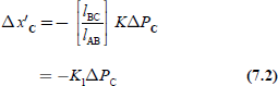
Equation (7.15) can be represented in a block diagram model as shown in Fig. 7.6, which is the linearized model of the speed-governor mechanism.
From the block diagram, ![]() is the net input to the speed-governor system and ΔxE(s) is the output of the speed governor.
is the net input to the speed-governor system and ΔxE(s) is the output of the speed governor.
7.12 TURBINE MODEL
We are interested not in the turbine valve position but in the generator power increment ΔPG. The change in valve position ΔxE causes an incremental increase in turbine power ΔPT and due to electromechanical interactions within the generator, it will result in an increased generator power ΔPG, i.e., ΔPT = ΔPG, since the generator incremental loss is neglected. This overall mechanism is relatively complicated particularly if the generator voltage simultaneously undergoes wild swing due to major network disturbances.
At present, we can assume that the voltage level is constant and the torque variations are small. Then an incremental analysis will give a relatively simple dynamic relationship between ΔxE and ΔPG. Such an analysis reveals considerable differences, not only between steam turbines and hydro-turbines, but also between various types (reheat and non-reheat) of steam turbines. Therefore, the transfer function, relates the change in the generated power output with respect to the change in the valve position, varies with the type of the prime mover.
7.12.1 Non-reheat-type steam turbines
Figure 7.7 (a) shows a single-stage non-reheat type steam turbine.
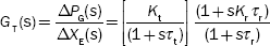
In this model, the turbine can be characterized by a single gain constant Kt and a single time constant τt as

FIG. 7.7 (a) Single-stage non-reheat-type steam turbine; (b) block diagram representation of a non-reheat-type steam turbine; (c) transfer function representation of speed control mechanism of a generator with a non-reheat-type steam turbine
Typically, the time constant τt lies in the range of 0.2 to 2.
On opening the steam valve, the steam flow will not reach the turbine cylinder instantaneously. The time delay experienced in this is in the order of 2 s in the steam pipe.
From Equation (7.16), we have
We can represent Equation (7.17) by a block diagram as shown in Fig. 7.7(b).
Figure 7.7(c) shows the linearized model of a non-reheat-type turbine controller including the speed-governor mechanism.
From Fig. 7.7(c), the combined transfer function of the turbine and the speed-governor mechanism will be ![]()
Therefore,
In general, it is obtained that the turbine response is low with the response time of several seconds.
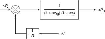
FIG. 7.8 Block diagram of a simplified turbine governor
7.12.2 Incremental or small signal for a turbine-governor system
Let the command incremental signal be ΔPC. Then in the steady state, we get ΔPG = KsgKtΔPC. Let KsgKt = 1; the block diagram of Fig. 7.7(c) is reduced to that shown in Fig. 7.8.
This block diagram gives the derivation of an incremental or small signal model. The model is adopted for large signal use by adding a saturation-type non-linear element, which introduces the obvious fact that the steam valve must operate between certain limits. The valve can neither be more open than fully open nor more closed than fully closed.
This model of Fig. 7.8 may also be modified to account for reheat cycles in the turbine and more accurate representation of fluid dynamics in the steam inlet pipes or in the hydraulic turbines in the penstock.
7.12.3 Reheat type of steam turbines
Modern generating units have reheat-type steam turbines as prime movers for higher thermal efficiency.
Figure 7.9 shows a two-stage reheat-type steam turbine.
In such turbines, steam at high pressure and low temperature is withdrawn from the turbine at an intermediate stage. It is returned to the boiler for resuperheating and then reintroduced into the turbine at low pressure and high temperature. This increases the overall thermal efficiency. Mostly, two factors influence the dynamic response of a reheat-type steam turbine:
- Entrained steam between the inlet steam valve and the first state of turbine.
- The storage action in the reheater, which causes the output of the low-pressure stage to lag behind that of the high-pressure stage.
FIG. 7.9 A two-stage reheat type of a steam turbine
Thus, in this case, the turbine transfer function is characterized by two time constants. It involves an additional time lag τr associated with the reheater in addition to the turbine time constant τt. Hence, the turbine transfer function will be of a second order and is given by
The time constant τr has a value in the range of 10 s and approximates the time delay for charging the reheat section of the boiler. Kr is a reheat coefficient and is equal to the proportion of torque developed in the high-pressure section of the turbine:
Kr = (1 – fraction of the steam reheated)
When there is no reheat Kr = 1 and the transfer function reduces to a single time constant given in Equation (7.16).
The transfer functions as given by Equations (7.16) and (7.18) give good representation within the first 20 s following the incremental disturbance. They do not account for the slower boiler dynamics. To get an easy analyzation, it can be assumed that the prime mover or turbine is modeled by a single equivalent time constant τt as given in Equation (7.16).
7.13 GENERATOR–LOAD MODEL
The generator–load model gives the relation between the change in frequency (Δf) as a result of the change in generation (ΔPG) when the load changes by a small amount (ΔPD).
When neglecting the change in generator loss, ΔPG = ΔPT (change in turbine power output), net-surplus power at the bus bar = (ΔPG – ΔPD). This surplus power can be absorbed by the system in two different ways:
(i) By increasing the stored kinetic energy of the generator rotor at a rate ![]()
Let W 0KE be the stored KE before the disturbance at normal speed and frequency f 0, and WKE be the KE when the frequency is (f 0 + Δf).
Since the stored KE is proportional to the square of speed and the frequency is proportional to the speed,
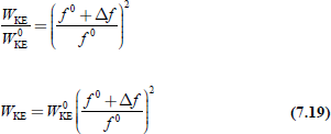
Neglecting higher-order terms, since ![]() is small:
is small:
Differentiating the above expression with respect to ‘t’, we get
Let H be the inertia constant of a generator (MW-s/MVA) and Pr the rating of the turbo-generator (MVA):
W0KE = H × Pr (MW-s or M-J) (7.22)
Hence, Equation (7.21) becomes
(ii) The load on the motors increases with increase in speed. The load on the system being mostly motor load, hence some portion of the surplus power is observed by the motor loads. The rate of change of load with respect to frequency can be regarded as nearly constant for small changes in frequency.
i.e.,
where the constant B is the area parameter in MW/Hz and can be determined empirically. B is positive for a predominantly motor load.
Now, the surplus power can be expressed as
From Equations (7.23) and (7.24), the above equation can be modified as
Dividing throughout by Pr of Equation (7.25), we get
Taking Laplace transform on both sides, we get


where ![]() is the power system time constant (normally 20 s) and
is the power system time constant (normally 20 s) and ![]() the power system gain.
the power system gain.
Equation (7.26) can be represented in a block diagram model as given in Fig. 7.10.
The overall block diagram of an isolated power system is obtained by combining individual block diagrams of a speed-governor system, a turbine system, and a generator–load model and is as shown in Fig. 7.11.
This representation being a third-order system, the characteristic equation for the system will be of the third order.

FIG. 7.10 Block diagram representation of a generator–load model

FIG. 7.11 Complete block diagram representation of an isolated power system
Example 7.1: Two generating stations 1 and 2 have full-load capacities of 200 and 100 MW, respectively, at a frequency of 50 Hz. The two stations are interconnected by an induction motor and synchronous generator set with a full-load capacity of 25 MW as shown in Fig. 7.12. The speed regulation of Station-1, Station-2, and induction motor and synchronous generator set are 4%, 3.5%, and 2.5%, respectively. The loads on respective bus bars are 750 and 50 MW, respectively. Find the load taken by the motor-generator set.
Solution:
Let a power of A MW flow from Station-1 to Station-2:
∴ Total load on Station-1 = (75 + A) MW
Total load on Station-2 = (50 − A)
% drop in speed at Station-1 = ![]()
% drop in speed at Station-2 = ![]()
The reduction in frequency will result due to the power flow from Station-1 through the interconnector of M-G set.
∴ % drop in speed at M-G set = ![]()
(reduction in frequency at Station-1 + reduction in frequency at M-G set)
= (reduction in frequency at Station-2)
![]()
0.02 (75 + A) + 0.1A |
= |
0.035 (50 − A) |
1.5 + 0.02A + 0.1A |
= |
1.75 − 0.03A |
0.02A + 0.1A + 0.03A |
= |
175 − 1.5 = 0.25 |
0.15A |
= |
0.25 |
A |
= |
1.666 MW |
i.e., a power of A |
= |
1.666 MW fl ows from Station-1 to Station-2. |
∴ Total load at Station-1 = 75 + A |
= |
75 + 1.666 = 76.666 MW |
Total load at Station-2 = 50 − A |
= |
50 − 1.666 = 48.334 MW |
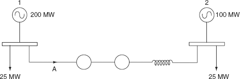
FIG. 7.12 Illustration for Example 7.1
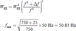
Example 7.2: A 125 MVA turbo-alternator operator on full load operates at 50 Hz. A load of 50 MW is suddenly reduced on the machine. The steam valves to the turbine commence to close after 0.5 s due to the time lag in the governor system. Assuming the inertia to be constant, H = 6 kW-s per kVA of generator capacity, calculate the change in frequency that occurs in this time.
Solution:
By defi nition, ![]()
∴ Energy stored at no load = 6 × 125 × 1,000 = 750 MJ
Excessive energy input to rotating parts in 0.5 s = 50 × 0.5 × 1,000 = 25 MJ
As a result of this, there is an increase in the speed of the motor and hence an increase in frequency:
7.14 CONTROL AREA CONCEPT
In real practice, the system of a single generator that feeds a large and complex area has rarely occurred. Several generators connected in parallel, located also at different locations, will meet the load demand of such a geographically large area. All the generators may have the same response characteristics to the changes in load demand.
It is possible to divide a very large power system into sub-areas in which all the generators are tightly coupled such that they swing in unison with change in load or due to a speed-changer setting. Such an area, where all the generators are running coherently is termed as a control area. In this area, frequency may be same in steady state and dynamic conditions. For developing a suitable control strategy, a control area can be reduced to a single generator, a speed governor, and a load system.
7.15 INCREMENTAL POWER BALANCE OF CONTROL AREA
In this section, we shall develop a dynamic model in terms of incremental power and frequency dynamics of a control area ‘i’ connected via tie lines as shown in Fig. 7.13.
Now assume that control area ‘i’ experiences a real load change ΔPDi (MW). Due to the actions of the turbine controllers, its output increases by ΔPGi (MW). The net-surplus power in the area (ΔPGi – ΔPDi) will be absorbed by the system in three ways:
- By increasing the area kinetic energy WKE, i at the rate

- By an increased load consumption. All typical loads (because of the dominance of motor loads) experience an increase,
 with speed or frequency.
 - By increasing the flow of power via tie lines with the total amount ΔPtie, i MW, which is defined positive for outflow from the area.

FIG. 7.13 Interconnected control area
Hence, the net-surplus power can be expressed as
ΔPtie is the difference between scheduled real power and actual real power through interconnected lines and it is taken as the input to the LFC system.
7.16 SINGLE AREA IDENTIFICATION
The first two terms on the right-hand side of Equation (7.27) represent a generator–load model (with the subscript ‘i’ absent). If the third term is absent, it means that there is no interchange of power between area ‘i’ and any other area. Thus, it becomes a single-area case. A single area is a coherent area in which all the generators swing in unison to the changes in load or speed-changer settings and in which the frequency is assumed to be constant throughout both in static and dynamic conditions. This single control area can be represented by an isolated power system consisting of a turbine, its speed governor, generator, and load.
7.16.1 Block diagram representation of a single area
The block diagram of an isolated power system, which in essence is a single-area system, is the same as the block diagram given in Fig. 7.11.
7.17 SINGLE AREA—STEADY-STATE ANALYSIS
The block diagram of an LFC of an isolated power system of a third-order model is represented in Fig. 7.11.
There are two incremental inputs to the system and they are:
- The change in the speed-changer position, ΔPC (reference power input).
- The change in the load demand, ΔPD.
In this section, we will analyze the response of a single-area system to steady-state changes by three ways:
- Constant speed-changer position with variable load demand (uncontrolled case).
- Constant load demand with variable speed-changer position (controlled case).
- Variable speed-changer position as well as load demand.
7.17.1 Speed-changer position is constant (uncontrolled case)
With the model given in Fig. 7.11 and with ΔPC = 0, the response of an uncontrolled single area LFC can be obtained as follows.
Let us consider a simple case wherein the speed changer has a fixed setting, which means ΔPC = 0 and the load demand alone changes. Such an operation is known as free governor operation or uncontrolled case since the speed changer is not manipulated (or controlled to achieve better frequency constancy).
For a sudden step change of load demand,
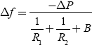
For such an operation, the steady-state change of frequency Δ f is to be estimated from the block diagram of Fig. 7.14 as
Applying the final value theorem, we have

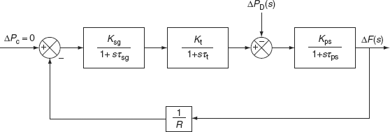
FIG. 7.14 Block diagram representation of an isolated power system setting ΔPC = 0
The gain Kt is fixed for the turbine and Kps is fixed for the power system. The gain Ksg of the speed governor is easily adjustable by changing the lengths of various links of the linkage mechanism. Ksg is so adjusted such that KsgKt ≈ 1.
Therefore Equation (7.29) can be simplified as:

Also we know from the dynamics of the generator–load model, ![]()
where ![]()
![]() in p.u.MW/unit change in frequency
in p.u.MW/unit change in frequency
where the factor ![]() and is known as the area frequency response characteristic (AFRC) or area frequency regulation characteristic.
and is known as the area frequency response characteristic (AFRC) or area frequency regulation characteristic.
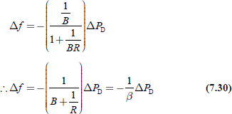
Equation (7.30) gives the steady-state response of frequency to the changes in load demand. The speed regulation is usually so adjusted that changes in frequency are small (of the order of 5%) from no load to full load. Figure 7.15 gives the linear relationship between frequency and load for a free governor operation, with speed changes set to give a scheduled frequency of 100% at full load.
The droop or the slope of the relationship is ![]()
Power system parameter B is generally much less than ![]() so that B can be neglected in Equation (7.30), which results in
so that B can be neglected in Equation (7.30), which results in
The droop of the frequency curve is thus mainly determined by the speed-governor regulation (R).
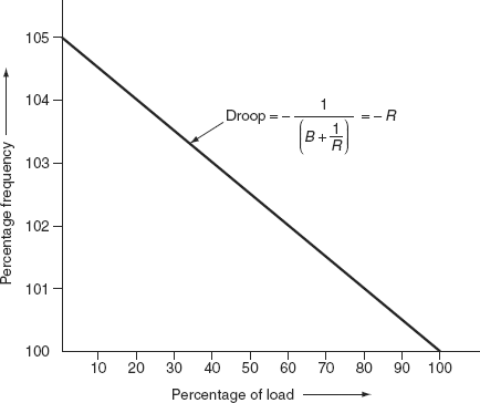
FIG. 7.15 Steady-state load frequency characteristics of a speed-governing system
The increase in load demand (ΔPD) is met under steady-state conditions partly by the increased generation (ΔPG) due to the opening of the steam valve and partly by the decreased load demand due to droop in frequency.
The increase in generation is expressed as
Substituting Δf from Equation (7.30), we get

And a decrease in the system load is expressed as
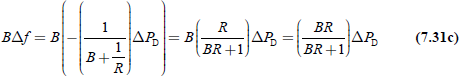
From Equations (7.31(b)) and (7.31(c)), it is observed that contribution of the decrease in the system load is much less than the increase in generation.
7.17.2 Load demand is constant (controlled case)
Consider a step change in a speed-changer position with the load demand remaining fixed:
i.e., ![]()
The steady-state change in frequency can be obtained from the block diagram of Fig. 7.16:

The steady-state value is obtained by applying the final-value theorem:

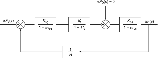
FIG. 7.16 Block diagram representation of an isolated power system setting ΔPD = 0
7.17.3 Speed changer and load demand are variables
By superposition, if the speed-changer setting is changed by ΔPc while the load demand also changes by ΔPD, the steady-state change in frequency is obtained from Equations (7.30) and (7.32) as
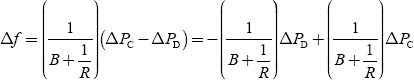
From the above equation, we can observe that the change in load demand causes the changes in frequency, which can be compensated by changing the position of the speed changer.
If ΔPC = ΔPD, then Δf will become zero.
7.18 STATIC LOAD FREQUENCY CURVES
The block diagram representation of a turbine-speed-governor model is shown in Fig. 7.17(a) and their static load frequency curves are shown in Fig. 7.17(b).
The curve relates power generation PG and frequency f with control parameter PC.
From the block diagram shown in Fig. 7.17(a), we get the static algebraic relation from which the local shape of the speed-power curves may be inferred.
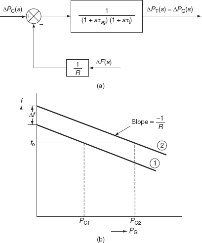
FIG. 7.17 (a) Block diagram of a turbine-speed-governor model; (b) static load frequency curves for the turbine governor
Figure 7.17(b) gives the two static load-frequency curves. Adjust power generation, PG, by using a speeder meter (speed changer) upto PG = PC1, where PC1 is the desired command power at synchronous speed ω0 (f 0). With free governor operation (i.e., ΔPC = 0), the fixed speed-changer position PC1 predicts the straight-line relationship. This straight line (1) has a slope of – R.
To get more generation at the same synchronous speed of ω0 (f 0), adjust PC1 to PC2 with a speeder meter. This results in the load frequency curve (2). The speed regulation R refers to the variation in frequency with power generation. Better the regulation results, less the droops speed-power (load) characteristics of LFC.
7.19 DYNAMIC ANALYSIS
The meaning of dynamic response is how the frequency changes as a function of time immediately after disturbance before it reaches the new steady-state condition. The analyzation of dynamic response requires the solution of dynamic equation of the system for a given disturbance. The solution involves the solution of different equations representing the dynamic behavior of the system.
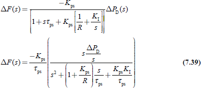
The inverse Laplace transform of ΔF(s) gives the variation of frequency with respect to time for a given step change in load demand. Comparing the relative values of time constants, we can reduce the third ordered model to a first ordered system.
For a practical LFC system,
τsg < τt << τPs
Typical values are:
τsg = 0.4 s
τt = 0.5 s
τPs = 20 s
If τsg and τt are considered negligible compared to τPs and by adjusting Ksg Kt = 1, the block diagram of LFC of the power system of an isolated system is reduced to a first-order system as shown in Fig. 7.18 with ΔPc = 0 for an uncontrolled case.
From Fig. 7.18, the change in frequency is given by
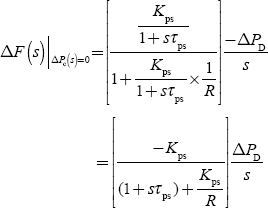

FIG. 7.18 First-order approximate block diagram of LFC of an isolated area
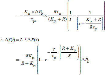

FIG. 7.19 Dynamic response of frequency change (Δf) for a step-load change
The plot of change in frequency versus time for a first-order approximation and exact response are shown in Fig. 7.19:
ΔPD = 0.01 p.u, Kps = 100, R = 3, τsg = 0.4 s, τt = 0.5 s, and τPs = 20 s
Example 7.3: An isolated control area consists of a 200-MW generator with an inertia constant of H = 5 kW-s/kVA having the following parameters (Fig. 7.20(a)):
Power system gain constant, Kps = 100
Power system time constant, τps = 20 s
Speed regulation, R = 3
Normal frequency, f 0 = 50 Hz
Obtain the frequency error and plot the graph of deviation of frequency when a step-load disturbance of (i) 0.5%, (ii) 1%, and (iii) 2% is applied (Fig. 7.20(b)).
From Fig. 7.20(b), the steady-state change in frequency Δfss = –0.0145 Hz.
Similarly (ii) for a step-load change of 1%, the steady-state change in frequency Δfss = –0.029 Hz; (iii) for a step-load change of 2%, steady-state change in frequency Δfss = –0.0583 Hz
Example 7.4: For Example 7.3, show the effect of governor action and turbine dynamics (Fig. 7.21(a)), if they are not to be neglected and given that τsg = 0.4 s and τt = 0.5 s for a step-load change of (i) 0.5% and (ii) 1% (Fig. 7.21(b)).
From Fig. 7.21(b), the steady-state change in frequency Δfss = –0.0235 Hz.
Similarly (ii) for a step-load change of 1%, the steady-state change in frequency Δfss = –0.047 Hz.
Example 7.5: Obtain the resultant frequency plot when combining Examples 7.3 and 7.4 for a step-load disturbance of 0.5% (Figs. 7.22(a) and (b)).
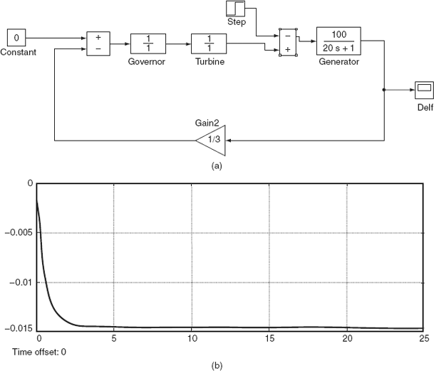
FIG. 7.20 (a) Simulation block diagram of single area without a speed-governor system; (b) response of the change in frequency for Fig. 7.20(a) for a step-load change of 0.5%

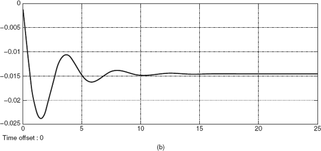
FIG. 7.21 (a) Simulation block diagram of single area with a speed-governor system; (b) response of the change in frequency for Fig. 7.21(a) for a step-load change of 0.5%


FIG. 7.22 (a) Simulation block diagram of a single area without and with a speed-governor system; (b) response of the change in frequency for Fig. 7.22(a) for a step-load change of 0.5%
Example 7.6: An isolated control area consists of a 200-MW generator with an inertia constant of H = 5 kw-s/kVA having the following parameters (Fig. 7.23(a)):
Power system gain constant, Kps = 100
Power system time constant, τps = 20s
Speed regulation, R = 3
Normal frequency, f 0 = 50 Hz
Governor time constant, τsg = 0.4 s
Turbine time constant, τt = 0.5 s
Obtain the frequency error and plot the graph of deviation of frequency when a step change of 1% in the speed-changer position is applied (Fig. 7.23(b)).


FIG. 7.23 (a) Simulation block diagram of a simulated system with a step change in the speed-changer position; (b) frequency response for Example 7.6
Example 7.7: An isolated control area consists of a 200-MW generator with an inertia constant of H = 5 kW-s/kVA having the following parameters (Fig. 7.24(a)):
Power system gain constant, Kps = 100
Power system time constant, τps = 20 s
Speed regulation, R = 3
Normal frequency, f 0 = 50 Hz
Governor time constant, τsg = 0.4 s
Turbine time constant, τt = 0.5 s
Obtain the frequency error and plot the graph of deviation of frequency when a step change of 1% in both the speed-changer position and the load is applied (Fig. 7.24(b)).
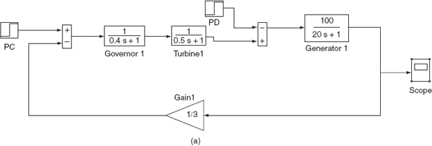

FIG. 7.24 (a) Simulation block diagram of a single-area system with PC and PD ; (b) frequency response of Example 7.5
Example 7.8: Find the static frequency drop if the load is suddenly increased by 25 MW on a system having the following data:
Rated capacity Pr = 500 MW
Operating Load PD = 250 MW
Inertia constant H = 5 s
Governor regulation R = 2 Hz p.u. MW
Frequency f = 50 Hz
Also find the additional generation.
Solution:
Assuming the frequency characteristic to be linear, we have
![]()
∂PD/∂f expressed in p.u., ![]()
![]()
Area frequency response characteristic (AFRC)
![]()
The static frequency drop ![]()
Hence, the system frequency drops to (50 – 0.098) = 49.902 Hz.
The amount of additional generation

While the sudden increase in load is 25 MW, the increase in generation is 24.5 MW and 0.5 MW is the loss of load due to the drop in frequency.
7.20 REQUIREMENTS OF THE CONTROL STRATEGY
The following are the basic requirements needed for the control strategy:
- The system frequency control is obtained through a closed loop. Since stability is the major problem associated with a closed-loop control, maintenance of the stability will be the main objective.
- The frequency deviation due to a step-load change should return to zero. The control that offers above is called ‘isochronous control’. In addition, the control should keep the magnitude of the transient frequency deviation to a minimum.
- The integral of the frequency error should not exceed a certain maximum value.
Isochronous control ensures that the steady-state frequency error following a step-load change will be zero. However, no control can eliminate transient frequency error. The time error of synchronous clocks is proportional to the integral of this transient frequency error. Therefore, it is necessary to put a limit on the value of this integral.
- The total load should be divided among the individual generators of the control area for optimum economy.
The first three requirements are satisfied when the addition of the integral-control to the system takes place.
7.20.1 Integral control
The integral control is composed of a frequency sensor and an integrator. The frequency sensor measures the frequency error Δf and this error signal is fed into the integrator. The input to the integrator is called the ‘Area Control Error’ (i.e., ACE = Δf).
The ACE is the change in area frequency, which when used in an integral-control loop, forces the steady-state frequency error to zero.
The integrator produces a real-power command signal ΔPC and is given by
|
ΔPC = −KI ∫ Δf dt |
(7.33) |
|
= −KI ∫ (ACE) dt |
|
The signal ΔPC is fed to the speed-changer causing it to move. Here, KI is called the integral gain constant, which controls the rate of integration. The frequency sensor and the integrator are connected in the system as a closed control loop as shown in the block diagram in Fig. 7.25.
Figure 7.25 consists of Fig. 7.11 augmented by additional loops showing the generation of ACE and its use in changing the area command powers; R is the speed-regulation feedback parameter. ΔPG(s), ΔPD(s), and ΔF(s) are the incremental changes in the generation, system load, and frequency, respectively. The block diagram of Fig. 7.25 is the single-area power system (isolated power system) with integral control for small incremental changes.
The negative sign in the integral controller is for producing a negative or decrease command for a positive frequency error. The gain constant KI is positive and controls the rate of integration, and thus the speed of the response of the control loop. The integrator is an electronic integrator of the same type as used in analog computers.
In view of hardware, we can understand the presence of the integrator by considering the ACE voltages distributed to the speed changers (speeder motors) of individual generator units that participate in supplementary control within a given area. These motors turn at a rate of θ proportional to the ACE voltage and continue to turn until they are driven to zero.

FIG. 7.25 Proportional plus integral control of LFC of a single-area system
The integral control will give rise to zero steady-state frequency error (Δfsteady state = 0) due to a step-load change. As long as the error remains, the integrator output will increase, causing the speed changer to move. The integrator output and thus the speed-changer position attain a constant value only when the frequency error has been reduced to zero. This is proved through a simplified mathematical analysis as follows.
7.21 ANALYSIS OF THE INTEGRAL CONTROL
The following assumptions are made in order to obtain a simple analysis. These assumptions do not distort the essential features. Also, the errors introduced on account of these assumptions affect only the transient and not the steady-state response.
Assumptions
- The time constant of the speed-governor mechanism τsg and that of the turbine τt are both neglected, i.e., τsg = τt = 0.
- The speed changer is an electromechanical device and hence its response is not instantaneous. However, it is assumed to be instantaneous in the present analysis.
- All non-linearities in the equipment, such as dead zone, etc., are neglected.
- The generator can change its generation ΔPG as fast as it is commanded by the speed changer.
- The ACE is a continuous signal.
The Laplace transformation of Equation (7.33) gives
and, for a step change of load demand ΔPD,
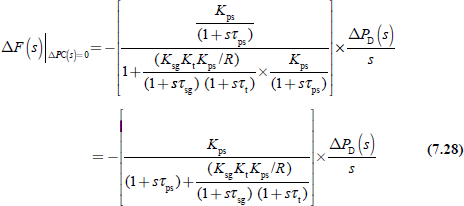
From the block diagram of Fig. 7.25, we have

and

Substituting for ΔPG(s) from Equation (7.36) in the above equation, we get

Equation (7.38) becomes a fourth-order system.
The steady-state value of Δf (t) can be obtained by applying the final-value theorem, viz.,
Hence, the static- or steady-state frequency error will be zero with integral control.
The nature of transient variation of Δf (t) can be found by taking the inverse Laplace transform of Equation (7.39). According to assumption (i), Equation (7.39) simplifies to
The nature of Δf (t) depends on the roots of the characteristic equation of Equation (7.39)
The above equation can be rewritten as

where  is a positive real number
and 
The nature of the roots of Equation (7.41) depends on whether ω 2 = 0, ω 2 > 0, or ω 2 < 0.
Case (i): ω 2 = 0
The characteristic equation has a repeated root (viz., α repeated twice). Hence, the expression for Δf (t) contains terms of the type
e–αt and t e–αt
Consequently, the response [viz., Δf (t)] is a critically damped one. For this critical case,

Solving the above for KI, we get

Case (ii): ω 2 > 0
Now, (s + α)2 = –ω 2, where ω 2 is a positive real number.
(s + α) = + jω
(or) s = (– α ± jω)
The time response Δf (t) will therefore consist of damped oscillatory terms of the type
e–αt sin ωt and e–αt cos ωt.
This case is called a supercritical case. In this case, KI > KIcrit.
Case (iii): ω 2 > 0
Then, ω 2 is a negative real number.
So, (s + α)2 = –ω 2 is a positive real number
= γ2 (say)
∴ (s + α) = + γ [since γ < α]
or s = (−α + γ) or (−α − γ)
= β1 or − β2 (say)
Accordingly, in this case, the time response Δf (t) will comprise terms of the type
e−β1t and e−β2t
Hence, the response will be damped and non-oscillatory. The control, in this case, is called the subcritical integral control. In this case, KI < KIcrit.
In all the three cases described above, Δf (t) will approach zero. This was proved earlier using the final-value theorem. It can be observed that the transient frequency error does remain finite. This is a proof that the control is both stable and isochronous. Thus, the first two control requirements stated earlier (Section 7.20) are fulfilled with this integral control. This control is also called ‘proportional plus integral control’. The proportional control is provided by the closed loop of gain constant of 1/R.
The actual simulated time responses of a single-area control system with and without integral control are as shown in Fig. 7.26.
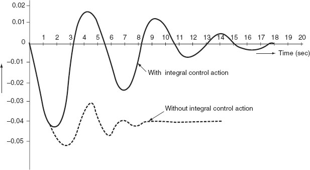
FIG.7.26 Dynamic response of LFC of a single-area system with and without integral control action
7.22 ROLE OF INTEGRAL CONTROLLER GAIN (KI) SETTING
The role played by the gain setting of an integral controller in the control of frequency error is described below.
With subcritical in gain settings (i.e., KI < KIcrit), a sluggish, non-oscillatory response is obtained. The slowness of the response makes the integral of Δf (t), and hence the time error, relatively large. However, with this setting, the generator need not ‘chase’ rapid load fluctuations, which ultimately cause equipment wear.
7.23 CONTROL OF GENERATOR UNIT POWER OUTPUT
The collective performance of all generators in the system is studied by assuming the equivalent generator having an inertia constant of Heq to be equal to the sum of the inertia constants of all the generating units. Similarly, the effects of the system loads are lumped into a single damping constant B.
For a system having ‘n’ generators and a composite load-damping constant of B the steady-state frequency deviation following a load change ΔPD is

The composite frequency response characteristic of the system is
It is normally expressed in MW/Hz. Sometimes, it is referred to as the stiffness of the system.
Example 7.9: An isolated control area consists of a 200-MW generator with an inertia constant of H = 5 kW-s/kVA having the following parameters (Fig. 7.27(a)):
Power system gain constant, Kps = 104
Power system time constant, τps = 22 s
Speed regulation, R = 3
Normal frequency, f 0 = 50 Hz
Governor time constant, τsg = 0.3 s
Turbine time constant, τt = 0.4 s
Obtain the frequency error and plot the graph of deviation of frequency when a step-load change of 0.48 p.u. with an integral controller action of ki = 0.1 is applied (Fig. 7.27(b)).
Example 7.10: An isolated control area consists of a 200-MW generator with an inertia constant of H = 5 kW-s/kVA having the following parameters (Fig. 7.28(a)):
Power system gain constant, Kps = 100
Power system time constant, τps = 20 s
Speed regulation, R = 2.5
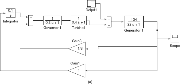
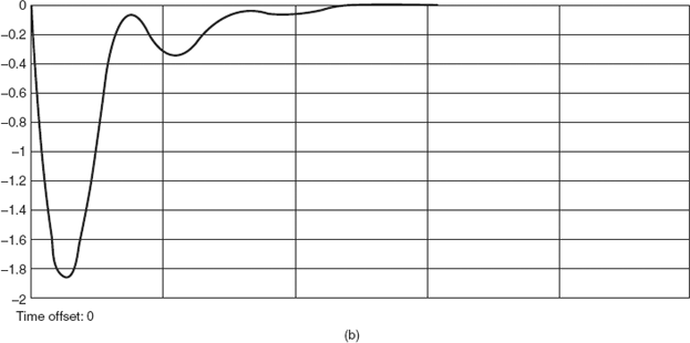
FIG. 7.27 (a) Simulation block diagram for a single-area system with integral control action; (b) frequency response characteristics of Example 7.9
Normal frequency, f 0 = 50 Hz
Governor time constant, τsg = 0.3 s
Turbine time constant, τt = 0.4 s
Integrator gain constant, ki = 0.15
Obtain the frequency error and plot the graph of deviation of frequency when a step-load disturbance of 2% with and without the integral control action is applied (Fig. 7.28(b)).
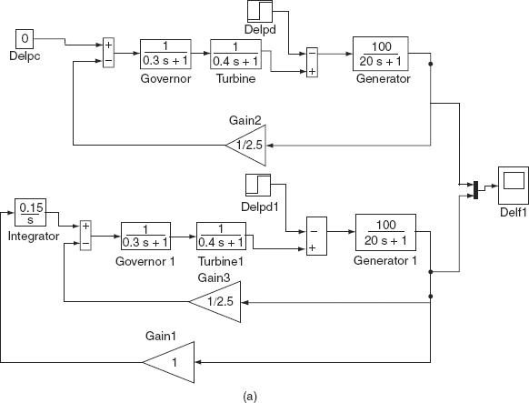

FIG. 7.28 (a) Simulation diagram of a single-area system without and with integral control action; (b) frequency response characteristics of Example 7.10
Example 7.11: Given a single area with three generating units as shown in Fig. 7.29:
| Unit | Rating (MVA) | Speed droop R (per unit on unit base) |
|---|---|---|
1 |
100 |
0.010 |
2 |
500 |
0.015 |
3 |
500 |
0.015 |
The units are loaded as P1 = 80 MW; P2 = 300 MW; P3 = 400 MW. Assume B = 0; what is the new generation on each unit for a 50-MW load increase? Repeat with B = 1.0 p.u. (i.e., 1.0 p.u. on load base).
Solution:

with B = 0; at a common base of 1,000 MVA

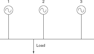
FIG. 7.29 A single area with three generating units
f = f 0 + Δf
= 50 − 652.17 × 10⁻⁶ (50) = 49.96 Hz
Changes in unit generation:

New generation:
P1′ = P1 + ΔP1 = 80 + 6.52 = 86.52 MW
P2′ = P2 + ΔP2 = 300 + 21.74 = 321.74 MW
P3′ = P3 + ΔP3 = 400 + 21.74 = 421.74 MW
- with B = 1 p.u. (on load base)

Changes in unit generation:

New generation:
P1′ = P1 + ΔP1 = 80 + 6.44 = 86.44 MW
P2′ = P2 + ΔP2 = 300 + 21.459 = 321.459 MW
P3′ = P3 + ΔP3 = 400 + 21.459 = 421.459 MW
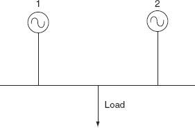
FIG. 7.30 Single area with two generating units
Example 7.12: Given a single area with two generating units as shown in Fig. 7.30:
| Unit | Rating (MVA) | Speed droop R (per unit on unit base) |
|---|---|---|
1 |
400 |
0.04 |
2 |
800 |
0.05 |
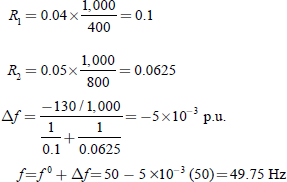
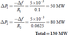
The units share a load of P1 = 200 MW; P2 = 500 MW. The units are operating in parallel, sharing 700 MW at 1.0 (50 Hz) frequency. The load is increased by 130 MW.
With B = 0, find the steady-state frequency deviation and the new generation on each unit.
With B = 0.804, find the steady-state frequency deviation and the new generation on each unit.
Solution:
At a common base of 1,000 MVA:
Change in unit generation:
New generation:
P1′ = P1 + ΔP1 = 200 + 50 = 250 MW
P2′ = P2 + ΔP2 = 500 + 80 = 580 MW
- With B = 0.804 (on load base)

Change in unit generation:

New generation:
P1′ = P1 + ΔP1 = 200 + 48.5 = 248.5 MW
P2′ = P2 + ΔP2 = 500 + 77.6 = 577.6 MW
Example 7.13: A 500-MW generator has a speed regulation of 4%. If the frequency drops by 0.12 Hz with an unchanged reference, determine the increase in turbine power. And also find by how much the reference power setting should be changed if the turbine power remains unchanged.
Solution:
Case 1:
Speed regulation,

![]()
Given a drop in frequency, Δf = –0.12 Hz
Increase in turbine power,

∴ Turbine power increase, ΔP = 30 MW
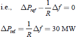
Case 2:
If the turbine power remains unchanged, the reference power setting at the point of the block diagram must be changed such that the signal to the increase in generation is blocked:
Example 7.14: Two generating units having the capacities 600 and 900 MW and are operating at a 50 Hz supply. The system load increases by 150 MW when both the generating units are operating at about half of their capacity, which results in the frequency falling by 0.5 Hz. If the generating units are to share the increased load in proportion to their ratings, what should be the individual speed regulations? What should the regulations be if expressed in p.u. Hz/p.u. MW?
Solution:
Rated capacity of Unit-1 = 600 MW
Rated capacity of Unit-2 = 900 MW
System frequency, f = 50 Hz
System load increment, ΔP = 150 MW
Falling in frequency, Δf = 0.5 Hz
We know that ![]()
If the load is shared in proportional to their ratings,
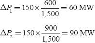
∴ From Equation (7.43),
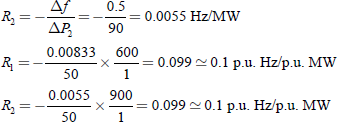
It is observed that the speed regulations in p.u. Hz/p.u. MW are attaining the same value, even when they are based on their individual ratings and they have different regulations.
Example 7.15: A single-area system has the following data:
Speed regulation, R = 4 Hz/p.u. MW
Damping coefficient, B = 0.1 p.u. MW/Hz
Power system time constant, TP = 10 s
Power system gain, KP = 75 Hz/p.u. MW
When a 2% load change occurs, determine the AFRC and the static frequency error. What is the value of the steady-state frequency error if the governor is blocked?
Solution:

Static frequency error

If the governor is blocked, the feedback loop will not be present; therefore, R will become infinite:

Static frequency error

i.e., frequency falls by 0.0571 Hz.
∴ New frequency, f′ = 50 − 0.0571
= 49.94 Hz
Observation:
With speed-governor action:
Frequency falls by 0.0571 Hz
∴ New frequency, f ′ = 50 – 0.0571
= 49.94 Hz
Without speed-governor action:
Frequency falls by 0.2 Hz
∴ New frequency, f ′ = 50 – 0.2 = 49.8 Hz
From the above results, it is noted that the speed-governor action is necessary for obtaining a reduction in the steady-state frequency error.
Example 7.16: A 200-MVA synchronous generator is operated at 3,000 rpm, 50 Hz. A load of 40 MW is suddenly applied to the machine and the station valve to the turbine opens only after 0.4 s due to the time lag in the generator action. Calculate the frequency to which the generated voltage drops before the steam flow commences to increase so as to meet the new load. Given that the valve of H of the generator is 5.5 kW-s per kVA of the generator energy.
Solution:
Given:
Rating of the generator = 200 MVA
Load applied on the m/c = 40 MW
Time taken by the valve to open = 0.4 s
H = 5.5 kW-s/kVA
= 11 × 105 s
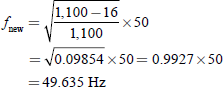
Energy stored at no-load = 5.5 × 200 ×1,000 = 1,100 MW-s = 1,100 MJ
Before the steam valve opens, the energy lost by the rotor = 40 × 0.4 = 16 MJ.
The energy lost by the rotor results in a reduction in the speed of the rotor and hence the reduction in frequency.
We know
![]()
∴ Frequency at the end of 0.4 s =
Example 7.17: Two generators of rating 100 and 200 MW are operated with a droop characteristic of 6% from no load to full load. Determine the load shared by each generator, if a load of 270 MW is connected across the parallel combination of those generators.
Solution:
The two generators are operating with parallel connection; the % drop in frequency from two generators due to different loads must be same.
Let power supplied by (100 MW) Generator-1 = x
Percentage drop in frequency = 6%
∴Percentage drop in the speed of Generator-1![]()
Total load across the parallel connection = 270 MW
Power supplied by (200 MW) Generator-2 = (270 – x)
∴Percentage drop in the speed of Generator-2 ![]()
Percent drop in frequency (or speed) of both machines must be the same:
![]()
By solving the above equation, we get
x = 90 MW
∴ Load shared by Generator-1 (100 MW unit) = 90 MW
Load shared by Generator-2 (200 MW unit) = 270 – x
KEY NOTES
- Necessity of maintaining frequency constant
- All the AC motors should be given a constant frequency supply so as to maintain the speed constant.
- In continuous process industry, it affects the operation of the process itself.
- For synchronous operation of various units in the power system network, it is necessary to maintain the frequency constant.
- Frequency affects the amount of power transmitted through interconnecting lines.
- Load frequency control (LFC) is the basic control mechanism in the power system operation whenever there is a variation in load demand on a generating unit momentarily if there is an occurrence of unbalance between real-power input and output. This difference is being supplied by the stored energy of the rotating parts of the unit.
- Prime movers driving the generators are fitted with governors, which are regarded as primary control elements in the LFC system. Governors sense the change in a speed control mechanism to adjust the opening of steam valves in the case of steam turbines and the opening of water gates in the case of water turbines.
- The steady-state speed regulation in per unit is given by

The value of R varies from 2% to 6% for any generating unit.
- The speed governor is the main primary tool for the LFC, whether the machine is used alone to feed a smaller system or whether it is a part of the most elaborate arrangement.
Its main parts are fly-ball speed governor, hydraulic amplifier, speed changer, and linkage mechanism.
- Control area is possible to divide a very large power system into sub-areas in which all the generators are tightly coupled such that they swing in unison with change in load or due to a speed-changer setting. Such an area, where all the generators are running coherently is termed as a control area.
- A single area is a coherent area in which all the generators swing in unison to the changes in load or speed-changer settings and in which the frequency is assumed to be constant throughout both in static and dynamic conditions.
- Dynamic response is how the frequency changes as a function of time immediately after disturbance before it reaches the new steady-state condition. The canalization of dynamic response requires the solution of a dynamic equation of the system for a given disturbance.
- Integral control consists of a frequency sensor and an integrator. The frequency sensor measures the frequency error Δf and this error signal is fed into the integrator. The input to the integrator is called the ‘area control error (ACE)’.
- The ACE is the change in area frequency, which when used in an integral-control loop forces the steady-state frequency error to zero.
SHORT QUESTIONS AND ANSWERS
- What is the effect of speed of a generator on its frequency?
The effect of speed of a generator on its frequency is

where p is the number of poles and N the speed in rpm.
- Why should the system frequency be maintained constant?
Constant frequency is to be maintained for the following functions:
- All the AC motors should be given constant frequency supply so as to maintain the speed constant.
- In continuous process industry, it affects the operation of the process itself.
- For synchronous operation of various units in the power system network, it is necessary to maintain the frequency constant.
- What is the nature of the generator–load frequency characteristic?
The nature of the generator is drooping straight-line characteristics.
- How do load frequency characteristics change during on-line control?
By shifting the load frequency characteristics as a whole up or down varying the inlet valve opening of the prime mover.
- How do load frequency characteristics change during off-line control?
By changing the slope of the load characteristics by varying the lever ratio of the speed governor.
- State why P–f and Q–V control loops can be treated as non-interactive?
The active power P is mainly dependent on the internal angle δ and is independent of bus voltage magnitude |V|. The bus voltage is dependent on machine excitation and hence on reactive power Q and is independent of the machine angle δ. The change in the machine angle δ is caused by a momentary change in the generator speed and hence the frequency. Therefore, the load frequency and excitation voltage controls are non-interactive for small changes and can be modeled and analyzed independently.
- What will be the order of the system for non-reheat steam turbine and reheat turbine?
The order of the system for non-reheat and reheat steam turbine are first order and second order, respectively.
- What are the transfer functions of non-reheat steam turbine and reheat turbine? What will be the value of their time constants?
The transfer function of non-reheat type of steam turbine is

The transfer function of reheat type of steam turbine is
The time constant τr has a value in the range of 10 s.
- Under what condition will the model developed for a turbine be valid?
The condition for the turbine is the first 20 s following the incremental disturbance.
- Explain the control area concept.
It is possible to divide a very large power system into sub-areas in which all the generators are tightly coupled such that they swing in unison with change in load or due to a speed-changer setting. Such an area, where all the generators are running coherently, is termed the control area. In this area, frequency may be same in steady-state and dynamic conditions. For developing a suitable control strategy, a control area can be reduced to a single generator, a speed governor, and a load system.
- What is meant by single-area power system?
A single area is a coherent area in which all the generators swing in unison to the changes in load or speed-changer settings and in which the frequency is assumed to be constant throughout both in static and dynamic conditions. This single control area can be represented by an isolated power system consisting of a turbine, its speed governor, generator, and load.
- What is meant by dynamic response in LFC?
The meaning of dynamic response is how the frequency changes as a function of time immediately after disturbance before it reaches the new steady-state condition.
- What is meant by uncontrolled case?
For uncontrolled case, ΔPC = 0; i.e., constant speed-changer position with variable load.
- What is the need of a fly-ball speed governor?
This is the heart of the system, which controls the change in speed (frequency).
- What is the need of a speed changer?
It provides a steady-state power output setting for the turbines. Its upward movement opens the upper pilot valve so that more steam is admitted to the turbine under steady conditions. This gives rise to higher steady-state power output. The reverse happens for downward movement of the speed changer.
- What is meant by area control error?
The area control error (ACE) is the change in area frequency, which when used in an integral-control loop forces the steady-state frequency error to zero.
- What is the nature of the steady-state response of the uncontrolled LFC of a single area?
The nature of the steady-state response of a single area is the linear relationship between frequency and load for free governor operation.
- How and why do you approximate the system for the dynamic response of the uncontrolled LFC of a single area?
The characteristic equation of the LFC of an isolated power system is third order, dynamic response that can be obtained only for a specific numerical case.
However, the characteristic equation can be approximated as first order by examining the relative magnitudes of the different time constants involved.
- What are the basic requirements of a closed-loop control system employed for obtaining the frequency constant?
The basic requirements are as follows:
- Good stability;
- Frequency error, accompanying a step-load change, returns to zero;
- The magnitude of the transient frequency deviation should be minimum;
- The integral of the frequency error should not exceed a certain maximum value.
- What are the basic components of an integral controller
It consists of a frequency sensor and an integrator.
- Why should the integrator of the frequency error not exceed a certain maximum value?
The frequency error should not exceed a maximum value so as to limit the error of synchronous clocks.
- What are the assumptions made in the simplified analysis of the integral control?
- The time constant of the speed-governing mechanism τsg and that of the turbine are both neglected, i.e., it is assumed that τsg = τt = 0.
- The speed changer is an electromechanical device and hence its response is not instantaneous. However, it is assumed to be instantaneous in the present analysis.
- All non-linearities in the equipment, such as dead zone, etc., are neglected.
- The generator can change its generation ΔPG as fast as it is commanded by the speed-changer.
- The ACE is a continuous signal.
- State briefly how the time response of the frequency error depends upon the gain setting of the integral control.
If KI is less than its critical value, then the response will be damped non-oscillatory. Δf(t) reduces to zero in a longer time. Hence, the response is sluggish. This is an overdamped case. This is the subcritical case of integral control.
If KI is greater than its critical value, the time response would be damped oscillatory. Δf(t) approaches zero faster. This is an underdamped case. This is the supercritical case of the control.
If KI equals its critical value, no oscillations would be present in the time response and Δf(t) approaches zero in less time than in the subcritical case. The integral of the frequency error would be the least in this case.
MULTIPLE-CHOICE QUESTIONS
- If the load on an isolated generator is increased without increasing the power input to the prime mover:
- The generator will slow down.
- The generator will speed up.
- The generator voltage will increase.
- The generator field.
- Governors of controlling the speed of electric-generating units normally provide:
- A flat-speed load characteristic.
- An increase in speed with an increasing load.
- A decrease in speed with an increasing load.
- None
- When two identical AC-generating units are operated in parallel on governor control, and one machine has a 5% governor droop and the other a 10% droop, the machine with the greater governor droop will:
- Tend to take the greater portion of the load changes.
- Share the load equally with the other machine.
- Tend to take the lesser portion of the load changes.
- None.
- On LFC installations, error signals are developed proportional to the frequency error. If the frequency declines, the error signal will act to:
- Increase the prime mover input to the generators.
- Reduce the prime mover input to the generators.
- Increase generator voltages.
- None.
- If KE reduces
- w decreases.
- Speed falls.
- Frequency reduces.
- All.
- The changing of slope of a speed governer characteristic is achevied by changing the ratio of lever L of governer and can be made during
- On-line condition only.
- Off-line condition only.
- Both (a) and (b).
- Either (a) or (b).
- Unit of R is ________.
- Hz/MVAr.
- Hz/MVA.
- Hz/MW.
- Hz-s.
- Unit of B is ________.
- MVAr/Hz.
- MVA/Hz.
- MW/Hz.
- MW-s.
- Unit of H of a synchronous machine is:
- MJ/MW.
- MJ/MVA.
- MJ/s.
- MW-s.
- KE and frequency of a synchronous machine are related as:
- Input signals to an ALFC loop is ________.
- ΔPref
- ΔPD
- Both (a) and (b).
- None of these.
- Two main control loops in generating stations are:
- ALFC.
- AVR.
- Both (a) and (b).
- None of these.
- The speed regulation can be expressed as
- Ratio of change in frequency from no-load to full load to the rated frequency of the unit.
- Ratio of change in frequency to the corresponding change in real-power generation.
- (a) and (b).
- None of these.
- In an ALFC loop, Δf can be reduced using ________ controller.
- Differential.
- Integral.
- Proportional.
- All of these.
- Time constant of a power syste when compared to a speed governor is:
- Less.
- More.
- Same.
- None of these.
- Δf is of the order of ________ Hz.
- 0 to 0.05.
- –0.05 to 0.
- Both (a) and (b).
- None of these.
- In a power system ________ are continuously changing.
- Active and reactive power generation.
- Active and reactive power demands.
- Voltage and its angle.
- All of these.
- In a normal state, the frequency and voltage are kept at specified values that carefully maintain a balance between:
- Real-power demand and real-power generation.
- Reactive power demand and reactive power generation.
- Both.
- None of these.
- Real-power balance will control the variations in ________.
- Voltage.
- Frequency.
- Both.
- None of these.
- The excitations of the generators must be continuously regulated:
- To match the reactive power generations with reactive power demand.
- To control the variations in voltage.
- Both.
- None of these.
- ________ is the basic control mechanism in the power system.
- LFC.
- Voltage.
- Both.
- None of these
- Setting of speed-load characteristic parallel to itself is known as ________ and its adapted as on-line control.
- Primary control.
- Supplementary control.
- Basic.
- All of these.
- The basic function of LFC is:
- To maintain frequency for variations in real-power demand.
- To maintain voltage for variations in reactive power demand.
- To maintain both voltage and frequency for variations in real-power demand.
- To maintain both voltage and frequency for variations in real-power demand.
- The degree of unbalance between real-power generation and real-power demand is indicated by the index:
- Speed regulation R.
- Change in voltage,
- Frequency error.
- None.
- The LFC system ________ in the system.
- Does consider the reactive power flow.
- Does not consider the reactive power flow.
- Does not consider the real-power flow.
- ________ controls the excitation voltage and modifies the excitation.
- Change in real-power, ΔPa.
- Change in frequency Δ.
- Change in tie-line power, ΔPtie.
- Change in reactive power ΔQci.
- The p–f controller is employed to:
- Control the frequency.
- Monitor the active power flows in interconnection.
- Control the voltage.
- Only (a).
- Only (b).
- (b) and (c).
- (a) and (b).
- Which of the following is correct regarding p–f controller?
- It senses the frequency error.
- It changes the tie-line powers.
- Provides the information about incremental error in power angle Δδ.
- (a) and (b).
- (b) and (c).
- (a) and (c).
- All of these.
- The control signal that will change the position of the inlet valve of the prime mover is:
- ΔPci.
- ΔPgi.
- ΔPdi.
- None of these.
- The objective of Q–V controller is to transform the:
- Terminal voltage error signal into a reactive power control signal, ΔQci.
- Terminal voltage error signal into a real-power control signal, ΔPci.
- Frequency error signal into a real-power control signal, ΔPci.
- None of these.
- The active power P is:
- Mainly dependent on the internal torque angle, δ.
- Almost independent of the voltage magnitude.
- totally dependent on both the torque angle and the voltage.
- Mainly dependent on voltage and independent of torque angle, δ.
- (a) and (d).
- (b) and (c).
- (a) and (b).
- Only (d).
- The bus voltage V is:
- Dependent on the internal torque angle, δ.
- Almost independent of active power, P.
- Dependent on machine excitation and hence on reactive power.
- Almost independent of internal torque angle, δ.
- and (d).
- (b) and (c).
- (a) and (b).
- (c) and (d).
- Usually p–f controller and Q–V controller for ________ change, can be considered as ________ type.
- Dynamic, non-interacting.
- Static, interacting.
- Static, non-interacting.
- None of these.
- AVR loop is ________ control mechanism.
- Slow.
- Faster.
- Slow in some cases and faster in some other cases.
- None of these.
- ALFC loop is ________ control mechanism.
- Slow.
- Faster.
- Slow as well as fast.
- None of these.
- Which of the following indicates the large-signal analysis of power system dynamics?
- Large and sudden variations in the system variables due to sudden disturbances.
- Mathematical model is a set of non-linear differential equations.
- Mathematical model is a set of linear differential equations.
- Small and gradual variations of system variables.
- (a) and (b).
- (b) and (c).
- (c) and (d).
- None of these.
- Laplace transform methods are employed to determine the response of the system in ________ analysis.
- Large signal.
- Small signal.
- Both.
- None of these.
- A signal area system is one in which:
- It is not connected to any other system.
- Total demand on the system should be fully met by its own local generation.
- All generators swing together.
- All of these.
- In a signal area system, all generators working remain in synchronism maintaining their relative power angles; such a group of generators is called ________.
- Swing group.
- Synchro group.
- Coherent group.
- None of these.
- The heart of the speed governor system, which controls the change in speed is:
- Linkage mechanism.
- Fly-ball speed governor.
- Speed changer.
- Hydraulic amplifier.
- In a hydraulic amplifier:
- High-power-level pilot valve moment is converted into low-power-level main piston movement.
- Low-power pilot valve moment is converted into low-power-level piston movement.
- Low-power-level pilot valve moment is converted into high-power-level piston movement.
- Low-power-level pilot valve moment is converted into high-power-level pilot valve moment.
- Linkage mechanism provides:
- The moment of control valve in propositional to the inlet steam.
- The feedback from the control valve moment.
- Both (a) and (b).
- None of these.
- The primary control loop in generator control is:
- Linkage mechanism.
- Fly-ball speed governor.
- Speed changer.
- Hydraulic amplifier.
- The position of the pilot valve can be affected through linkage mechanism in ________ way.
- For non-reheat type of steam turbine, the mathematical model is:


- None of these.
- In reheat type of steam turbine,
- Steam at high pressure with low temperature is transformed into steam at low pressure with higher temperature.
- Steam at low pressure with higher temperature is transformed into steam at high pressure with low temperature.
- Steam at low pressure with low temperature is transformed into steam at high pressure with higher temperature.
- None of these.
- Transfer function of reheat type of steam turbine is of ________ order.
- First.
- Second.
- Third.
- None of these.
- Transfer function of non-reheat type of steam turbine is of ________ order.
- First.
- Second.
- Third.
- None of these.
- The surplus power (ΔPG – ΔPD) can be absorbed by a system:
- By increasing the stored K Є of the system at the rate

- By motor loads.
- There is no absorption of surplus power by the system.
- Both (a) and (b).
- By increasing the stored K Є of the system at the rate
- The block diagram of the LFC of an isolated power system is of ________ model.
- First.
- Second.
- Third.
- Fourth.
REVIEW QUESTIONS
- Develop the block diagram of the LFC of a single-area system.
- Compare the steady state and dynamic operations of an isolated system.
- Draw the schematic diagram of a speed-governing system and explain its components on the dynamic response of an uncontrolled system with necessary equations. Hence, obtain the transfer function of a speed-governing system.
- How do the governor characteristics of the prime mover affect the control of system frequency and system load?
- Explain why it is necessary to maintain the frequency of the system constant.
- What do you mean by LFC?
- Draw a neat sketch of a typical turbine speed-governing system and derive its block diagram representation.
- For a single-area system, show that the static error in frequency can be reduced to zero using frequency control and comment on the dynamic response of an uncontrolled system with necessary equations.
- Explain the p–f and Q–V control loops of power system.
- What is meant by control area and ACE?
- Explain clearly about proportional plus integral LFC with a block diagram.
- Discuss the adverse effects of change in the voltage and the frequency of a power system. Mention the acceptable ranges of these changes.
PROBLEMS
- A 250-MVA synchronous generator is operating at 1,500 rpm, 50 Hz. A load of 50 MW is suddenly applied to the machine and the station valve to the turbine opens only after 0.35 s due to the time lag in the generator action. Calculate the frequency at which the generated voltage drops before the steam flow commences to increase to meet the new load. Given that the valve of H of the generator is 3.5 kW-s per kVA of the generator energy.
- Two generating stations A and B have full-load capacities of 250 and 100 MW, respectively. The interconnector connecting the two stations has an induction motor/synchronous generator (Plant C) of full-load capacity 30 MW; percentage changes of speeds of A, B, and C are 4, 3, and 2, respectively. The loads on bus bars A and B are MW and 50 MW, respectively. Determine the load taken by Plant C and indicate the direction of the power flow.
- A 750-MW generator has a speed regulation of 3.5%. If the frequency drops by 0.1 Hz with an unchanged reference, determine the increase in turbine power. And also find by how much the reference power setting should be changed if the turbine power remains unchanged.