
9
Reactive Power Compensation
OBJECTIVES
After reading this chapter, you should be able to:
- know the need of reactive power compensation
- discuss the objectives of load compensation
- discuss the operation of uncompensated and compensated transmission lines
- discuss the concept of sub-synchronous resonance (SSR)
- study the voltage-stability analysis
9.1 INTRODUCTION
In an ideal AC-power system, the voltage and the frequency at every supply point would remain constant, free from harmonics and the power factor (p.f.) would remain unity. For the optimum performance at a particular supply voltage, each load could be designed such that there is no interference between different loads as a result of variations in the current taken by each one.
Most electrical power systems in the world are interconnected to achieve reduced operating cost and improved reliability with lesser pollution. In a power system, the power generation and load must balance at all times. To some extent, it is self-regulating. If an unbalance between power generation and load occurs, then it results in a variation in the voltage and the frequency. If voltage is propped up with reactive power support, then the load increases with a consequent drop in frequency, which may result in system collapse. Alternatively, if there is an inadequate reactive power, the system’s voltage may collapse.
Here, the quality of supply means maintaining constant-voltage magnitude and frequency under all loading conditions. It is also desirable to maintain the three-phase currents and voltages as balanced as possible so that underheating of various rotating machines due to unbalancing could be avoided.
In a three-phase system, the degree to which the phase currents and voltages are balanced must also be taken into consideration to maintain the quality of supply.
To achieve the above-mentioned requirements from the supply point of view as well as the loads, which can deteriorate the quality of supply, we need load compensation.
Load compensation is the control of reactive power to improve the quality of supply in an AC-power system by installing the compensating equipment near the load.
9.2 OBJECTIVES OF LOAD COMPENSATION
The objectives of load compensation are:
- p.f. Correction.
- Voltage regulation improvement.
- Balancing of load.
9.2.1 p.f. Correction
Generally, load compensation is a local problem. Most of the industrial loads absorb the reactive power since they have lagging p.f.’s. The load current tends to be larger than it is required to supply the real power alone. So, p.f. correction of load is achieved by generating reactive power as close as possible to the load, which requires it to generate it at a distance and transmit it to the load, as this results not only in a large conductor size but also in increased losses. It is desirable to operate the system near unity p.f. economically.
9.2.2 Voltage regulation improvement
All loads vary their demand for reactive power, although they differ widely in their range and rate of variation. The voltage variation is due to the imbalance in the generation and consumption of reactive power in the system. If the generated reactive power is more than that being consumed, voltage levels go up and vice versa. However, if both are equal, the voltage profile becomes flat. The variation in demand for reactive power causes variation (or regulation) in the voltage at the supply point, which can interfere with an efficient operation of all plants connected to that point. So, different consumers connected to that point get affected. To avoid this, the supply utility places bounds to maintain supply voltages within defined limits. These limits may vary from typically ± 6% averaged over a period of a few minutes or hours.
To improve voltage regulation, we should strengthen the power system by increasing the size and number of generating units as well as by making the network more densely interconnected. This approach would be uneconomic and would introduce problems such as high fault levels, etc. In practice, it is much more economic to design the power system according to the maximum demand for active power and to manage the reactive power by means of compensators locally.
9.2.3 Load balancing
Most power systems are three-phased and are designed for balanced operation since their unbalanced operation gives rise to wrong phase-sequence components of currents (negative and zero-sequence components). Such components produce undesirable results such as additional losses in motors, generators, oscillating torque in AC machines, increased ripples in rectifiers, saturation of transformers, excessive natural current, and so on. These undesirable effects are caused mainly due to the harmonics produced under an unbalanced operation. To suppress these harmonics, certain types of equipment including compensators are provided, which yield the balanced operation of the power system.
9.3 IDEAL COMPENSATOR
An ideal compensator is a device that can be connected at or near a supply point and in parallel with the load. The main functions of an ideal compensator are instantaneous p.f. correction to unity, elimination or reduction of the voltage regulation, and phase balance of the load currents and voltages. In performing these interdependent functions, it will consume zero power.
The characteristics of an ideal compensator are to:
- provide a controllable and variable amount of reactive power without any delay according to the requirements of the load,
- maintain a constant-voltage characteristic at its terminals, and
- should operate independently in the three phases.
9.4 SPECIFICATIONS OF LOAD COMPENSATION
The specifications of load compensation are:
- Maximum and continuous reactive power requirement in terms of absorbing as well as generation.
- Overload rating and duration.
- Rated voltage and limits of voltage between which the reactive power rating must not be exceeded.
- Frequency and its variation.
- Accuracy of voltage regulation requirement.
- Special control requirement.
- Maximum harmonic distortion with compensation in series.
- Emergency procedure and precautions.
- Response time of the compensator for a specified disturbance.
- Reliability and redundancy of components.
9.5 THEORY OF LOAD COMPENSATION
In this section, relationships between the supply system, the load, and the compensator were to be developed. The supply system, the load, and the compensator can be modeled in different ways. Here, the supply system is modeled as a Thevenin’s equivalent circuit with reactive power requirements. The compensator is modeled as a variable impedance /as a variable source (or sink) of reactive current / power. According to requirements, the selection of model used for each component can be varied.
The assumption made in developing the relationships between supply system, the load, and the compensator is that the load and system characteristics are static / constant (or) changing slowly so that phasor representation can be used.
9.5.1 p.f. Correction
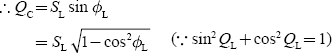
Consider a single-phase load with admittance YL = GL + jBL with a source voltage as shown in Fig. 9.1(a).
The load current IL is given by
IL = Vs (GL + jBL) = Vs GL + jVsBL = Ia + jIr
where Ia is the active component of the load current
Ir the reactive component of the load current.

FIG. 9.1 Representation of single-phase load; (a) without compensation; (b) with compensation
Apparent power of the load, SL |
= Vs IL* |
|
= VS2GL − jVS2 BL |
|
= PL + jQL |
where PL is the active power of the load
QL the reactive power of the load.
For inductive loads, BL is negative and QL is positive by convention.
The current supplied to the load is larger than when it is necessary to supply the active power alone by the factor
The objective of the p.f. correction is to compensate for the reactive power, i.e., locally providing a compensator having a purely reactive admittance jBC in parallel with the load as shown in Fig. 9.1(b). The current supplied from the source with the compensator is
Is |
= IL + IC |
|
= Vs (GL + jBL) – Vs (jBC) |
|
= VsGL = Ia (∵ BL = BC) |
which makes the p.f. to unity, since Ia is in phase with the source voltage Vs.
The current of the compensator, Ic = VsYc = –jVsBc
The apparent power of the compensator, Sc = VsIc*
Sc = jVs2 BC = −jQC (∵ SC = PC − jQC, for pure compensation PC = 0)
We know that
QL = PL tan ϕL
For a fully compensated system, i.e., QL=QC
The degree of compensation is decided by an economic trade-off between the capital cost of the compensator and the savings obtained by the reactive power compensation of the supply system over a period of time.
9.5.2 Voltage regulation
It is defined as the proportional change in supply voltage magnitude associated with a defined change in load current, i.e., from no-load to full load. It is caused by the voltage drop in the supply impedance carrying the load current.
When the supply system is balanced, it can be represented as single-phase model as shown in Fig. 9.2(a). The voltage regulation is given by ![]() , where |VL| is the load voltage.
, where |VL| is the load voltage.
9.5.2.1 Without compensator
From the phasor diagram of an uncompensated system, shown in Fig. 9.2(b), the change in voltages is given by
where Zs = Rs + jXs and the load current,
Substituting Zs and IL in Equation (9.1), we get
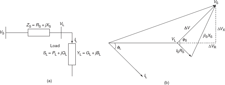
FIG. 9.2 (a) Circuit model of an uncompensated load and supply system; (b) phasor diagram for an uncompensated system
From Equation (9.3), it is observed that the change in voltage depends on both real and reactive powers of the load considering the line parameters to be constant.
9.5.2.2 With compensator
In this case, a purely reactive compensator is connected across the load as shown in Fig. 9.3(a) to make the voltage regulation zero, i.e., the supply voltage (|Vs|) equals the load voltage (|VL|). The corresponding phasor diagram is shown in Fig. 9.3(b).
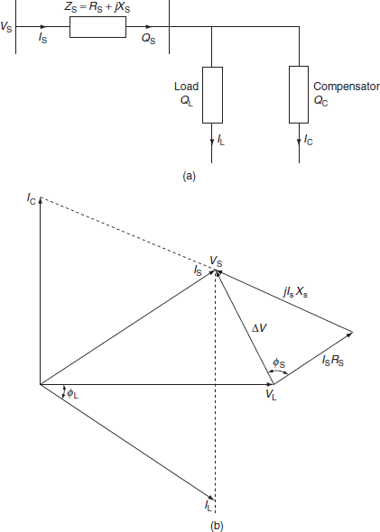
FIG. 9.3 (a) Circuit model of a compensated load and supply system; (b) phasor diagram for a compensated system
The supply reactive power with a compensator is
Qs = QC + QL
QC is adjusted in such a way that ∆V = 0
i.e., |Vs| = |VL|
From Equations (9.1) and (9.3), we get
Simplifying and rearranging equation (9.4),
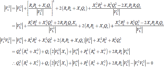
The above equation can be represented in a compact form as
a Qs2 + b Qs + c = 0
where
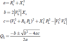
The value of QC is found using the above equation by using the compensator reactive power balance equation |Vs| = |VL| and QC = Qs – QL.
Here, the compensator can perform as an ideal voltage regulator, i.e., the magnitude of the voltage is being controlled, its phase varies continuously with the load current, whereas the compensator acting as a p.f. corrector reduces the reactive power supplied by the system to zero i.e., Qs = 0 = QL + QC.
Equation (9.3) can be reduced to
So, ∆V is independent of the load reactive power. From this, we conclude that a pure reactive compensator cannot maintain both constant voltage and unity p.f. simultaneously.
9.6 LOAD BALANCING AND P.F. IMPROVEMENT OF UNSYMMETRICAL THREE-PHASE LOADS
The third objective of load compensation is the balancing of unbalanced three-phase loads. We first model the load as a delta-connected admittance network for a general unbalanced three-phase load as shown in Fig. 9.4 in which the admittances YLab, YLbc and YLcd are complex and unequal.
In this case, supply voltages are assumed to be balanced. Any ungrounded Y-connected load can be represented by a delta-connected load by means of the Y-∆ transformation.
A compensator can be any passive three-phase admittance network, which when combined in parallel with the load will present a real and balanced load with respect to the supply.
9.6.1 p.f. Correction
Each load admittance can be made purely real by connecting, in parallel, a compensating susceptance equal to the negative of the load susceptance in that branch of the delta-connected load as shown in Fig. 9.5(a).
If load admittance, YLab = GLab + jBLab, then the compensating susceptance BCab = − BLab is connected across YLab:

An inductive susceptance between phases ‘c’ and ‘a’ as shown in Fig. 9.5(a) is

Now, the line currents will be balanced and are in phase with their respective phase voltages. The compensated single-phase load with a positive sequence equivalent circuit is shown in Fig. 9.5(a).

FIG. 9.4 Unbalanced three-phase load

FIG. 9.5 (a) Connection of p.f. correcting susceptance; (b) resultant unbalanced real load with unity p.f.
Similarly, the compensating susceptance, Bcbc = − BLbc and Bccd = − BLca are connected across YLbc and YLca, respectively, as shown in Fig. 9.5(a).
Figure 9.5(b) shows the resultant unbalanced real load with unity p.f.
9.6.2 Load balancing
Now, we make this real unbalanced load to a balanced one. To do this, let us consider a single-phase load (GLab) (as shown in Fig. 9.6(a)) of the ∆-connected load as shown in Fig. 9.5(b). The three-phase positive sequence line currents can be balanced by connecting capacitive susceptance between phases ‘b’ and ‘c’ and together with the inductive susceptance between phases ‘c’ and ‘a’ as shown in Fig. 9.6(b).
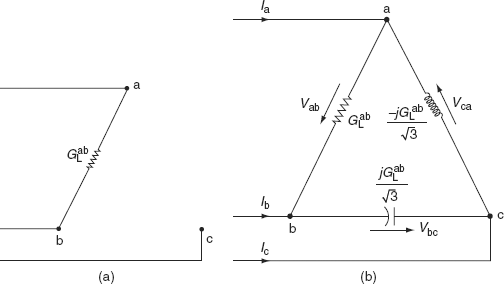
FIG. 9.6 (a) Single-phase unity p.f. load before positive sequence balancing; (b) positive sequence balancing of a single-phase u.p.f. load

FIG. 9.7 (a) Ideal three-phase compensating network with compensator admittances; (b) equivalent circuit of real and balanced compensated load admittance
Similarly, the real admittances in the remaining phases ‘bc’ and ‘ca’ can be balanced.
The resultant compensator admittance (susceptance) represented by an equivalent circuit is shown in Fig. 9.7(a).
Bcab = − BLab (p.f. correction) + (GLca + GLbc)/![]() (load balancing)
(load balancing)
Bcbc = − BLbc + (GLab + GLca)/![]()
Bcca = − BLca + (GLbc + GLab)/![]()
The resulting compensated load admittance is purely real and balanced, as shown in the equivalent circuit of Fig. 9.7(b).
9.7 UNCOMPENSATED TRANSMISSION LINES
An electric transmission line has four parameters, which affect its ability to fulfill its function as part of a power system and these are a series combination of resistance, inductance, shunt combination of capacitance, and conductance. These parameters are symbolized as R, L, C, and G, respectively. These parameters are distributed along the whole length at any line. Each small length at any section of the line will have its own values and concentration of all such parameters for the complete length of line into a single one is not possible. These are usually expressed as resistance, inductance, and capacitance per kilometer.
Shunt conductance that is mostly due to the breakage over the insulators is almost always neglected in a power transmission line. The leakage loss in a cable is uniformly distributed over the length of the cable, whereas it is different in the case of overhead lines. It is limited only to the insulators and is very small under normal operating conditions. So, it is neglected for an overhead transmission line.
9.7.1 Fundamental transmission line equation
Consider a very small element of length ∆x at a distance of x from the receiving end of the line. Let z be the series impedance per unit length, y the shunt admittance per unit length, and l the length of the line.

FIG. 9.8 Representation of a transmission line on a single-phase basis
Then,
Z = zl = total series impedance of the line
Y = yl = total shunt admittance of the line
The voltage and current at a distance x from the receiving end are V and I, and at distance x + ∆x are V + ∆V and I + ∆I, respectively (Fig. 9.8).
So, the change of voltage, ∆V = Iz∆x, where z∆x is the impedance of the element considered:

Similarly, the change of current, ∆I = Vy∆x, where y∆x is the admittance of the element considered:
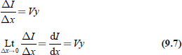
Differentiating Equation (9.6) with respect to x, we get
Substituting the value of ![]() from Equation (9.7) in Equation (9.8), we get
from Equation (9.7) in Equation (9.8), we get
Equation (9.9) is a second-order differentiatial equation and its solution is
Differentiating Equation (9.10) with respect to x, we get
From Equations (9.6) and (9.11), we have
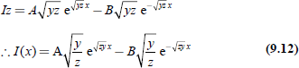
From Equation (9.10), we have
From Equation (9.12), we have
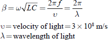
where ![]() is known as characteristic impedance or surge impedance and
is known as characteristic impedance or surge impedance and ![]() is known as the propagation constant.
is known as the propagation constant.
The constants A and B can be evaluated by using the conditions at the receiving end of the line.
The conditions are
at x = 0, V = Vr and I = Ir
Substituting the above conditions in Equations (9.11) and (9.12), we get
and
Solving Equations (9.15) and (9.16), we get
Now, substituting the values of A and B in Equations (9.13) and (9.14), then we get
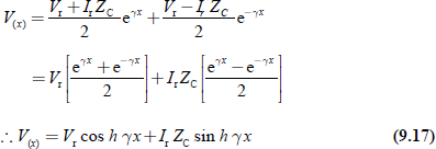

where V(x) and I(x) are the voltages and currents at any distance x from the receiving end.
For a lossless line γ = jβ and the hyperbolic functions, i.e., cos h γ x = cos h jβx = cos βx and sin h γ x = sin h jβx = j sin βx.
Therefore, Equations (9.17) and (9.18) can be modified as
and
where β is the electrical length of the line (radians or wavelength)
9.7.2 Characteristic impedance
The quantity ![]() is a complex number as y and z are in complex.
is a complex number as y and z are in complex.
It is denoted by ZC or Z0. It has the dimension of impedance, since
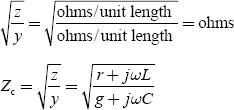
This quantity depends upon the characteristic of the line per unit length. It is, therefore, called characteristic impedance of the line. It also depends upon the length of the line, radius, and spacing between the conductors. For a lossless line, r = g = 0, the characteristic impedance becomes
The characteristic impedance is also called the surge or natural impedance of the line.
The approximate value of the surge impedance for overhead lines is 400 Ω and that for underground cables is 40 Ω, and the transformers have several thousand ohms as their surge impedance. Surge impedance is the impedance offered to the propagation of a voltage or current wave during its travel along the line.
9.7.3 Surge impedance or natural loading
The surge impedance loading (SIL) of a transmission line is the MW loading of a transmission line at which a natural reactive power balance occurs (zero resistance).
Transmission lines produce reactive power (MVAr) due to their natural capacitance. The amount of MVAr produced is dependent on the transmission line’s capacitive reactance (XC) and the voltage (kV) at which the line is energized.
Now the MVAr produced is
Transmission lines also utilize reactive power to support their magnetic fields. The magnetic field strength is dependent on the magnitude of the current flow in the line and the natural inductive reactance (XL) of the line. The amount of MVAr used by a transmission line is a function of the current flow and inductive reactance.
The MVAr used by a transmission line = I2XL (9.22)
Transmission line SIL is simply the MW loading (at a unity p.f.) at which the line MVAr usage is equal to the line MVAr production. From the above statement, the SIL occurs when

And the Equation (9.23) can be rewritten as

The term ![]() is the ‘surge impedance’.
is the ‘surge impedance’.
The theoretical significance of the surge impedance is that if a purely resistive load that is equal to the surge impedance were connected to the end of a transmission line with no resistance, a voltage surge introduced to the sending end of the line would be absorbed completely at the receiving end. The voltage at the receiving end would have the same magnitude as the sending-end voltage and would have a voltage phase angle that is lagging with respect to the sending end by an amount equal to the time required to travel across the line from the sending to the receiving end.
The concept of surge impedance is more readily applied to telecommunication systems rather than to power systems. However, we can extend the concept to the power transferred across a transmission line. The surge impedance loading (power transmitted at this condition) or SIL (in MW) is equal to the voltage squared (in kV) divided by the surge impedance (in ohms):
Note: In this formula, the SIL is dependent only on the voltage (kV) of the line is energized and the line surge impedance. The line length is not a factor in the SIL or surge impedance calculations. Therefore, the SIL is not a measure of a transmission line power transfer capability as it neither takes into account the line length nor considers the strength of the local power system.
The value of the SIL to a system operator is realized when a line is loaded above its SIL, it acts like a shunt reactor absorbing MVAr from the system and when a line is loaded below its SIL, it acts like a shunt capacitor supplying MVAr to the system.
9.8 UNCOMPENSATED LINE WITH OPEN CIRCUIT
In this section, we shall discuss the cases: (a) voltage and current profiles, (b) symmetrical line at no-load, and (c) underexcited operation of generators.
9.8.1 Voltage and current profiles
A lossless line is energized at the sending end and is open-circuited at the receiving end.
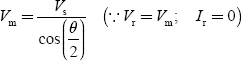
From Equations (9.19) and (9.20) with Ir = 0
Voltage and current at the sending end are given by equations with x = l as
V(x) = Vs, I(x) = I(s)
Equations (9.25) and (9.26) are modified as
where θ = βl
From Equations (9.25) and (9.26), the voltage profile equation is
And the current profi le equation,
9.8.2 The symmetrical line at no-load
This is similar to an open-circuited line energized at one end. This is a line identical at both ends, but with no power transfer. Suppose the terminal voltages are maintained as same values,
i.e., Vs = Vr
From Equations (9.19) and (9.20) with x = l, we have
The electrical conditions are the same (Vs = Vr); there would not be any power transfer. Therefore, by symmetry Is = Ir.
Substituting the above condition in Equations (9.32), we get
Substituting Equation (9.33) in Equation (9.31), we get

From Equation. (9.34), we have
A comparison of Equations (9.35) and (9.36) with Equation (9.28) shows that the line is equivalent to two equal halves connected back-to-back. Half the line-charging current is supplied from each end. By symmetry, the midpoint current is zero, whereas the midpoint voltage is equal to the open-circuit voltage of the line having half the total length.
From Equation (9.31) the midpoint voltage is
9.8.3 Underexcited operation of generators due to line-charging
No load at the receiving ends, i.e., Ir = 0. The charging reactive power at the sending end is
Qs = I m(VsIs*)
From Equation (9.28), we have
Line-charging current at the sending end, ![]()
∴ Line-charging power at the sending end, Qs = –P0 tan θ
For a 300-km line, Qs is nearly 43% of the natural load expressed in MVA. At 400 kV, the generators would have to absorb 172 MVAr.
The reactive power absorption capability of a synchronous machine is limited for two reasons:
- The heating of the ends of the stator core increases during underexcited operation.
- The reduced field current results in reduced internal e.m.f of the machine and this weakens the stability.
Using a compensator, this problem can be reduced by two ways:
- If the line is made up of two (or) more parallel circuits, one (or) more of the circuits can be switched off under light load (or) open-circuit conditions.
- If the generator absorption is limited by stability and not by core-end heating, the absorption limit can be increased by using a rapid response excitation system, which restores the stability margins when the steady-state field current is low. The underexcited operation of generators can set a more stringent limit to the maximum length of an uncompensated line than the open-circuit voltage rise.
9.9 THE UNCOMPENSATED LINE UNDER LOAD
In this section, the effects of line length, load power, and p.f. on voltage as well as reactive power are discussed.
9.9.1 Radial line with fixed sending-end voltage
A load (Pr + j Qr) at the receiving end of a radial line draws the current.
i.e., ![]()
From Equation (9.19), with x = l, for a lossless line, the sending-and receiving-end voltages are related as
If Vs is fixed, this quadratic equation can be solved for Vr. The solution gives how Vr varies with the load and its p.f. as well as with the line length.
Several fundamental important properties of AC transmission are evident from Fig. 9.9
- For each load p.f., there is a maximum transmissible power.
- The load p.f. has a strong influence on the receiving-end voltage.
- Uncompensated lines between about 150-km and 300-km long can be operated at normal voltage provided that the load p.f. is high. Longer lines, with large voltage variations, are impractical at all p.f.’s unless some means of voltage compensation is provided.
The midpoint voltage variation on a symmetrical 300-km line is the same as the receiving-end voltage variations on a 150-km line with a unity p.f. load.
9.9.2 Reactive power requirements
From the line voltage and the level of power transmission, the reactive power requirements can be determined. It is very important to know the reactive power requirements because they determine the reactive power ratings of the synchronous machines as well as those of any compensating equipment. If any inductive load is connected at the sending end of the line, it will support the synchronous generators to absorb the line-charging reactive power. With the absence of the compensating equipment, the synchronous machines must absorb or generate the difference between the line and the local load reactive powers.

FIG. 9.9 Magnitude of receiving-end voltage as a function of load and load p.f.
The equations of voltage and current for the sending-end half of the symmetrical line is
The power at midpoint is
Pm + j Qm = VmIm* = P = transmitted power
Since Qm = 0, because no reactive power flows at the midpoint.
The power at the sending end is
Ps + j Qs = VsIs*
Substituting Vs and Is from Equations (9.38) and (9.39) in the above equation, we get
If the line is assumed to be lossless, then Ps = Pr = P :

The above expression gives the relation between the midpoint voltage and the reactive power requirements of the symmetrical line.
If the terminal voltages are continuously adjusted so that the midpoint voltage,
Vm = V0 = 1.0 p.u. at all levels of power transmission

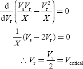
9.9.3 The uncompensated line under load with consideration of maximum power and stability
Consider Equation (9.37) as
If Vr is taken as reference phasor, then:
where δ is the phase angle between Vs and Vr and is called the load angle (or) the transmission angle.
Equating real and imaginary parts of Equations (9.40) and (9.41), we get
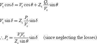
For an electrically short line, sin θ = θ = βl:
Then, ![]() the series reactance of the line:
the series reactance of the line:

where ![]()
9.10 COMPENSATED TRANSMISSION LINES
The change in the electrical characteristics of a transmission line in order to increase its power transmission capability is known as line compensation. While satisfying the requirements for a transmission system (i.e., synchronism, voltages must be kept near their rated values, etc.), a compensation system ideally performs the following functions:
- It provides the flat voltage profile at all levels of power transmission.
- It improves the stability by increasing the maximum transmission capacity.
- It meets the reactive power requirements of the transmission system economically.
The following types of compensations are generally used for transmission lines:
- Virtual-Z0.
- Virtual-θ.
- Compensation by sectioning.
The effectiveness of a compensated system is gauged by the product of the line length and maximum transmission power capacity. Compensated lines enable the transmission of the natural load over larger distances, and shorter compensated lines can carry loads more than the natural load.
The flat voltage profile can be achieved if the effective surge impedance of the line is modified as to a virtual value Z0′, for which the corresponding virtual natural load  is equal to the actual load. The surge impedance of the uncompensated line is
 ![]() , which can be written as
, which can be written as ![]() , if the series and /or the shunt reactance XL and/or Xc are modified, respectively. Then, the line can be made to have virtual surge impedance Z0′ and a virtual natural load P’ for which
, if the series and /or the shunt reactance XL and/or Xc are modified, respectively. Then, the line can be made to have virtual surge impedance Z0′ and a virtual natural load P’ for which
Compensation of line, by which the uncompensated surge impedance Z0 is modified to virtual surge impedance Z0′, is called virtual surge impedance compensation or virtual Z0 compensation.
Once a line is computed for Z0, the only way to improve stability is to reduce the effective value of θ. Two alternative compensation strategies have been developed to achieve this.
- Apply series capacitors to reduce XL and thereby reduce θ, since θ = βl =
 at fundamental frequency. This method is called line-length compensation (or) θ compensation.
 - Divide the line into shorter sections that are more (or) less independent of one another. This method is called compensation by sectioning. It is achieved by connecting constant voltage compensations at intervals along the line.
9.11 SUB-SYNCHRONOUS RESONANCE
In this section, various effects due to sub-synchronous resonance are discussed in detail.
9.11.1 Effects of series and shunt compensation of lines
The objective of series compensation is to cancel part of the series inductive reactance of the line using series capacitors, which results in the following factors.
- Increase in maximum transferable power capacity.
- Decrease in transmission angle for considerable amount of power transfer.
- Increase in virtual surge impedance loading.
From a practical point of view, it is desirable not to exceed series compensation beyond 80%. If the line is compensated at 100%, the line behaves as a purely resistive element and would result in series resonance even at fundamental frequency since the capacitive reactance equals the inductive reactance, and it would be difficult to control voltages and currents during disturbances. Even a small disturbance in the rotor angles of the terminal synchronous machine would result in flow of large currents.
The location of series capacitors is decided partly by economical factors and partly by the selectivity of fault currents as they would depend upon the location of the series capacitor. The voltage rating of the capacitor will depend upon the maximum fault current that likely flows through the capacitor.
The net inductive reactance of the line becomes
Xl net = Xl − Xsc
The connection of the transmission line and the series capacitor behaves like a series resonance circuit with inductive reactance of line in series with the capacitance of the series capacitor.
The effects of series and shunt compensation of overhead transmission lines are as follows:
- For a fixed degree of series compensation, the capacitive shunt compensation decreases the virtual surge impedance loading of the line. However, the inductive shunt compensation increases the virtual surge impedance and decreases the virtual surge impedance loading of the line.
- If the inductive shunt compensation is 100%, then the virtual surge impedance becomes infinite and the loading is zero, which implies that a flat voltage profile exists at zero loads and the Ferranti effect can be eliminated by the use of shunt reactors.
- Under a heavy-load condition, the flat voltage profile can be obtained by using shunt capacitors.
- A flat voltage profile can be obtained by series compensation for heavy loading condition.
- Voltage control using series capacitors is not recommended due to the lumped nature of series capacitors, but normally they are preferred for improving the stability of the system.
- Series compensation has no effect on the load-reactive power requirements of the generator and, therefore, the series-compensated line generates as much line-charging reactive power at no load as completely uncompensated line of the same length.
- If the length of the line is large and needs series compensation from the stability point of view, the generator at the two ends will have to absorb an excessive reactive power and, therefore, it is important that the shunt compensation (inductive) must be associated with series compensation.
9.11.2 Concept of SSR in lines
Consider a transmission line compensated by a series capacitors connection.
Let LL, Lg, and Lt be the inductance of the line, generator, and transformer, respectively. Let Csc be the capacitance of the series capacitor, XL the total inductive reactance (XL + Xg + Xt), and Xsc the reactance of the series capacitor.
The natural frequency of oscillation of the above-said series resonance circuit is given by the relation
The inductive reactance of the system is Xl = 2π f L
Capacitive reactance of the capacitor is ![]()
Therefore, the natural frequency of oscillation in terms of Xl and Xc is expressed as
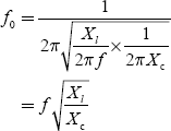
where f is the rated frequency.
The term ![]() represents the degree of series compensation and it varies between 25% and 65%; therefore, the natural frequency of oscillation becomes less when compared to the natural frequency (f0 < f), i.e., the series resonance will occur at sub-synchronous frequency.
represents the degree of series compensation and it varies between 25% and 65%; therefore, the natural frequency of oscillation becomes less when compared to the natural frequency (f0 < f), i.e., the series resonance will occur at sub-synchronous frequency.
There are three types of sub-synchronous oscillations that have been identified due to SSR conditions.
9.11.2.1 SSR due to induction generator effect
The transient currents at the sub-harmonic frequency resulted in a series-compensated network due to a switching operation or a fault. These sub-harmonic frequency currents assume dangerously high values and even become unstable. The unstable operation is exhibited in the form of a negative resistance in the equivalent circuit of synchronous and induction motors.
Considering a round-rotor synchronous machine, the sub-harmonic frequency operation can be studied with the help of its equivalent circuit as shown in Fig. 9.10.
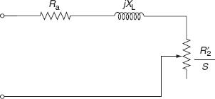
FIG. 9.10 Equivalent circuit of a synchronous machine for sub-harmonic operation
The sub-harmonic currents are excited in the stator winding of the synchronous machine due to some disturbances and these sub-harmonic currents would generally be unbalanced.
The positive sequence component of these unbalanced sub-harmonic currents will produce a magnetic field, which rotates in the same direction of rotation of the rotor but with a speed N < Ns. The machine behaves as an induction generator as far as sub-harmonic currents are considered. Due to this speed deviation between the rotor and the magnetic field, the slip ![]() will be present. Since f0 < f, the slip S becomes negative.
will be present. Since f0 < f, the slip S becomes negative.
Therefore, the equivalent resistance of the damper winding and the solid rotor resistance when referred to the stator side, i.e., ![]() becomes negative and therefore provides negative damping.
becomes negative and therefore provides negative damping.
If the series compensation is very high, the slip S would turn out to be very small and hence the equivalent resistance becomes very high and may become large enough to have total resistance of the system, which is negative. Therefore, it provides negative damping of the sub-harmonic currents, and voltage may build up to dangerously high values. Several measures are to be taken to prevent SSR in the system.
9.11.2.2 SSR due to torsional interaction between electrical and mechanical systems
The sub-harmonic currents produce field rotations in the direction with respect to the rotor and main field and which in turn produces an alternating torque on the rotor at the frequency (f –f0). If this frequency difference coincides with one of the natural tensional resonances of the machine shaft system, tensional oscillations may be excited and this operation is entirely known as SSR. It means that whenever the natural frequency of the mechanical oscillation of the rotor equals (f – f0), mechanical resonance would take place. Hence, SSR is treated as a combined electrical–mechanical resonance phenomenon.
The currents of high frequency may produce torque in some of the shafts, which may have the same natural frequency as the torque frequency (called swing frequency, which is the lowest frequency of natural oscillation of an equivalent system of a turbine cylinder and a generator) such that these shafts may break down due to the twisting action. Hence, resonant frequencies may be extended upto several hundreds of Hz. The large multiple-stage steam turbines that have more than one tensional modes in the frequency range of 0.5 Hz are more susceptible to SSR.
In the SSR phenomenon, if the resonance frequency coincides with the swing frequency, the whole turbine-generator assembly may come out from its foundation, and /or if the frequency of the torque developed coincides with the natural frequency of oscillation of some shafts and if oscillations build up sufficiently, it results in the breaking of the shaft.
9.11.2.3 SSR due to large disturbances
Due to the large disturbances like any switching operation or any fault condition, the condition of SSR occurs in the system even if oscillations are damped out. This SSR condition results in a ‘low cycle fatigue’ condition in a mechanical system or slow deterioration of the mechanical system due to the reduction in life of the shafts.
The corrective measures for SSR are:
- By passing a series of capacitors.
- Use of very sensitive relays to detect even small levels of sub-harmonic currents.
- Modulation of generator field current to provide an increased positive damping sub-harmonic frequency.
9.12 SHUNT COMPENSATOR
A shunt-connected static VAr compensator, composed of thyristor-switched capacitors (TSCs) and thyristor-controlled reactors (TCRs), is shown Fig. 9.11. With proper co-ordination of the capacitor switching and reactor control, the VAr output can be varied continuously between the capacitive and inductive rating of the equipment. The compensator is normally operated to regulate the voltage of the transmission system at a selected terminal, often with an appropriate modulation option to provide damping if power oscillation is detected.

FIG. 9.11 Static VAr compensator employing TSCs and TCR
9.12.1 Thyristor-controlled reactor
A shunt-connected thyristor-controlled inductor has an effective reactance, which is varied in a continuous manner by partial-conduction control of the thyristor valve.
With the increase in the size and complexity of a power system, fast reactive power compensation has become necessary in order to maintain the stability of the system. The thyristor-controlled shunt reactors have made it possible to reduce the response time to a few milliseconds. Thus, the reactive power compensator utilizing the thyristor-controlled shunt reactors become popular. An elementary single-phase TCR is shown Fig.9.12.
It consists of a fixed reactor of inductance L and a bidirectional thyristor valve. The thyristor valve can be brought into conduction by the application of a gate pulse to the thyristor, and the valve will be automatically blocked immediately after the AC current crosses zero. The current in the reactor can be controlled from maximum to zero by the method of firing angle control. Partial conduction is obtained with a higher value of firing angle delay. The effect of increasing the gating angle is to reduce the fundamental component of current. This is equivalent to an increase in the inductance of the reactor, reducing its current. As far as the fundamental component of current is concerned, the TCR is a controllable susceptance, and can, therefore, be used as a static compensator.
The current in this circuit is essentially reactive, lagging the voltage by 90° and this is continuously controlled by the phase control of the thyristors. The conduction angle control results in a non-sinusoidal current wave form in the reactor. In other words, the TCR generates harmonics. For identical positive and negative current half-cycle time, only odd harmonics are generated as shown in Fig. 9.13. By using filters, we can reduce the magnitude of harmonics.
TCR’s characteristics are:
- Continuous control.
- No transients.
- Generation of harmonics.

FIG. 9.12 TCR

FIG. 9.13 TCR waveform
9.12.2 Thyristor-switched capacitor
A shunt-connected TSC shows that an effective reactance is varied in a step-wise manner by full- or zero-conduction operation of the thyristor valve.
The TSC is also a sub-set of SVC in which thyristor-based AC switches are used to switch in and switch out shunt capacitors units in order to achieve the required step change in the reactive power supplied to the system. Unlike shunt reactors, shunt capacitors cannot be switched continuously with a variable firing angle control.
Depending on the total VAr requirement, a number of capacitors are used, which can be switched into or out of the system individually. The control is done continuously by sensing the load VArs. A single-phase TSC is shown in Fig. 9.14.
It consists of a capacitor, a bidirectional thyristor valve, and relatively small surge current in the thyristor valve under abnormal operating conditions (e.g., control malfunction causing capacitor switching at a ‘wrong time’); it may also be used to avoid resonance with system impendence at particular frequencies. The problem of achieving transient-free switching of the capacitors is overcome by keeping the capacitors charged to the positive or negative peak value of the fundamental frequency network voltage at all times when they are in the stand-by state. The switching-on-transient is then selected at the time when the same polarity exists in the capacitor voltage. This ensures that switching on takes place at the natural zero passage of the capacitor current. The switching thus takes place with practically no transients. This is called zero-current switching.

FIG. 9.14 TSC

FIG. 9.15 TSC waveforms
Switching off a capacitor is accomplished by suppression-offering pulses to the anti-parallel thyristors so that the thyristors will switch off as soon as the current becomes zero. In principle, the capacitor will then remain charged to the positive or negative peak voltage and be prepared for a new transient-free switching-on as shown in Fig. 9.15.
TSC’s characteristics are:
- Steeped control.
- No transients.
- No harmonics.
- Low losses.
- Redundancy and flexibility.
9.13 SERIES COMPENSATOR
In the TSC scheme, increasing the number of capacitor banks in series, controls the degree of series compensation. To accomplish this, each capacitor bank is controlled by a thyristor bypass switch or valve. The operation of the thyristor switches is co-ordinated with voltage and current zero-crossing; the thyristor switch can be turned on to bypass the capacitor bank when the applied AC voltage crosses zero, and its turn-off has to be initiated prior to a current zero at which it can recover its voltage-blocking capability to activate the capacitor bank. Initially, capacitor is charged to some voltage, while switching the SCR’s, they may get damaged because of this initial voltage. In order to protect the SCR’s from this kind of damage, resistor is connected in series with capacitor as shown in Fig. 9.16.
In a fixed capacitor, the TCR scheme as shown in Figs. 9.17 and 9.18, the degree of series compensation in the capacitive operating region is increased (or decreased) by increasing (or decreasing) the current in the TCR. Minimum series compensation is reached when the TCR is switched off. The TCR may be designed for a substantially higher maximum admittance at full thyristor conduction than that of the fixed shunt-connected capacitor. In this case, the TCR, time with an appropriate surge-current rating can be used essentially as a bypass switch to limit the voltage across the capacitor during faults and the system contingencies of similar effects.

FIG. 9.16 Series compensator
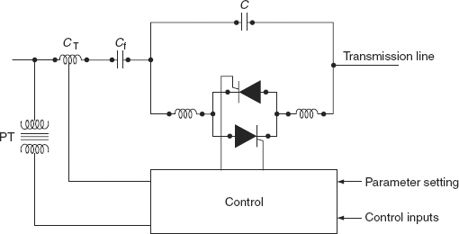
FIG. 9.17 Thyristor-controlled capacitor
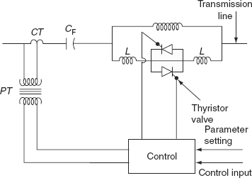
FIG. 9.18 TCR
Controllable series compensation can be highly effective in damping power oscillation and preventing loop flows of power.
The expression for power transferred is given by
![]()
where Vs is the sending-end voltage, Vr the receiving-end voltage, δ the angle between Vs and Vr, and X = XL – XC.
In interconnected power systems, the actual transfer of power from one region to another might take unintended routes depending on impedances of transmission lines connecting the areas. Controlled series compensation is a useful means for optimizing power flow between regions for varying loading and network configurations. It becomes possible to control power flows in order to achieve a number of goals that are listed below:
- Minimizing system losses.
- Reduction of loop flows.
- Elimination of line overloads.
- Optimizing load sharing between parallel circuits.
- Directing power flows along contractual paths.
9.14 UNIFIED POWER-FLOW CONTROLLER
In the UPFC, an AC voltage generated by a thyristor-based inverter is injected in series with the phase voltage. In Fig. 9.19, Converter-2 performs the main function of the UPFC by injecting, via., a series transformer, an AC voltage with controllable magnitude and a phase angle in series with the transmission line. The basic function of Converter-1 is to supply or absorb the real power demanded by Converter-2 at the common DC link. It can also generate or absorb controllable reactive power and provide an independent shunt-reactive compensation for the line. Converter-2 either supplies or absorbs the required reactive power locally and exchanges the active power as a result of the series injection voltage.

FIG. 9.19 The UPFC
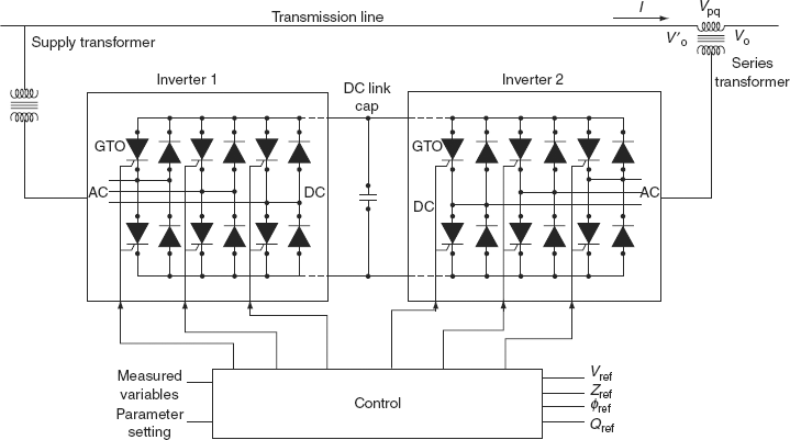
FIG. 9.20 Implementation of the UPFC using two voltage source inverters with a direct voltage link simultaneously
Generally, the impedance control would cost less and be more effective than the phase angle control, except where the phase angle is very small or very large or varies widely.
In general, it has three control variables and can be operated in different modes. The shunt-connected converter regulates the voltage bus ‘i’ in Fig. 9.20 and the series-connected converter regulates the active and reactive power or active power and the voltage at the series-connected node. In principle, a UPFC is able to perform the functions of the other FACTS devices, which have been described, namely voltage support, power-flow control, and an improved stability.
9.15 BASIC RELATIONSHIP FOR POWER-FLOW CONTROL
The basic concept of controlling power transmission in real time assumes the available means for rapidly changing those parameters of the power system, which determine the power flow. To consider the possibilities for a power-flow control, power relationships for the simple two-machine model are shown in Figs. 9.21 and 9.22.
Figure 9.22 shows the sending- and receiving-end generators with voltage phasors VS and Vr, inductive transmission line impedance (XL) in two sections ![]() , and generalized power-flow controller operated (for convenience) at the middle of the line. The power-flow controller consists of two controllable elements, i.e., a voltage source (Vxy) and a current source (Ix) are connected in series and shunt, respectively, with the line at the midpoint. Both the magnitude and the angle of the voltage Vxy are freely variables, whereas only the magnitude of current Ix is variable; its phase angle is fixed at 90° with respect to the reference phasor of midpoint voltage Vm. The basic power-flow relation is shown in Fig. 9.22 by using FACTS controller in a normal transmission system.
, and generalized power-flow controller operated (for convenience) at the middle of the line. The power-flow controller consists of two controllable elements, i.e., a voltage source (Vxy) and a current source (Ix) are connected in series and shunt, respectively, with the line at the midpoint. Both the magnitude and the angle of the voltage Vxy are freely variables, whereas only the magnitude of current Ix is variable; its phase angle is fixed at 90° with respect to the reference phasor of midpoint voltage Vm. The basic power-flow relation is shown in Fig. 9.22 by using FACTS controller in a normal transmission system.

FIG. 9.21 Simple two-machine power system with a generalized power-flow controller

FIG. 9.22 Power-flow relation
The four classical cases of power transmission are as follows:
- Without line compensation.
- With series capacitive compensation.
- With shunt compensation.
- With phase angle control,
They can be obtained by appropriately specifying Vxy and Ix in the generalized power-flow controller.
9.15.1 Without line compensation
Consider that the power-flow controller is off, i.e., both Vxy and Ix are zero. Then, the power transmitted between the sending- and receiving-end generators can be expressed by the well-known formula:
where δ is the angle between the sending- and receiving-end voltage phasors. Power P(1) is plotted against angle δ in Fig. 9.23.
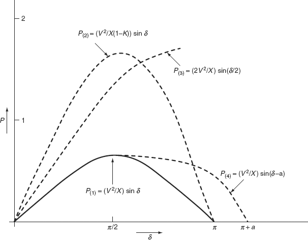
FIG. 9.23 The basic power transmission on characteristics for four different cases
9.15.2 With series capacitive compensation
Assume parallel current source, Ix = 0, and series voltage source, Vxy = – jn XLI, i.e., the voltage inserted in series with the line lags the line current by 90° with an amplitude that is proportional to the magnitude of the line current and that of the line impedance. In other words, the voltage source acts at the fundamental frequency precisely as a series- compensating capacitor. The degree of series compensating is defined by coefficient n (i.e., 0 ≤ n ≤ 1). With this, P against δ relationship becomes
9.15.3 With shunt compensation
Consider that series voltage source Vxy = 0 and parallel current source ![]() i.e., the current source Ix draws just enough capacitive current to make the magnitude of the midpoint voltage Vm equal to V. In other words, the reactive current source acts like an ideal shunt compensator, which segments the transmission line into two independent parts, each with an impedance of
i.e., the current source Ix draws just enough capacitive current to make the magnitude of the midpoint voltage Vm equal to V. In other words, the reactive current source acts like an ideal shunt compensator, which segments the transmission line into two independent parts, each with an impedance of ![]() by generating the reactive power necessary to keep the midpoint voltage constant, independently of angle δ. For this case of ideal midpoint compensation, the P against δ relation can be written as
by generating the reactive power necessary to keep the midpoint voltage constant, independently of angle δ. For this case of ideal midpoint compensation, the P against δ relation can be written as
9.15.4 With phase angle control
Assume that Ix = 0 and Vxy = ± jVm tan α, i.e., a voltage (Vxy) with the amplitude ± jVm tan α, is added in quadrature to the midpoint voltage (Vm) to produce the desired α phase shift. The basic idea behind the phase shifter is to keep the transmitted power at a desired level independently of angle δ in a pre-determined operating range. Thus, for example, the power can be kept at its peak value after angle δ is π/2 by controlling the amplitude of the quadrature voltage Vxy so that the effective phase angle (δ – α) between the sending- and receiving-end voltages stays at π/2. In this way, the actual transmitted power may be increased significantly even though the phase shifter does not increase the steady-state power transmission limit. Considering (δ – α) as the effective phase angle between the sending-end and the receiving-end voltage, the transmitted power can be expressed as
from Fig. 9.23, it can be seen that the power in without compensating is less shown in the P(1) curve. Power is increased by using the series capacitor compensation shown in the P(2) curve. The power angle curve with the shunt compensator is shown in the P(3) curve, in this case, power is increased and it seems that voltage is increased. The concept of the phase angle control is shown in the P(4) curve by shifting the curve higher, and power can be obtained.
9.16 COMPARISON OF DIFFERENT TYPES OF COMPENSATING EQUIPMENT FOR TRANSMISSION SYSTEMS
The comparison among different types of compensating equipment for transmission systems is tabulated below (Table 9.1).
TABLE 9.1 Comparison of different types of compensating equipment for transmission systems
| Compensating equipment | Advantages | Disadvantages |
|---|---|---|
Switched shunt reactor |
Simple in principle and construction |
Fixed in value |
Switched shunt capacitor |
Simple in principle and construction |
Fixed in value-switching transients. Required overvoltage protection and sub-harmonic filters. Limited overload capacity |
Series capacitor |
Simple in principle. Performance relatively sensitive to location. Has useful overload capability |
High-maintenance requirements. Slow control response |
Compensating equipment |
Advantages |
Disadvantages |
Synchronous condenser |
Fully controllable. Low harmonics |
Performance sensitive to location. Requires strong foundations |
Polyphase-saturated reactor |
Very rugged construction. Large overload capability. No effect on fault level. Low harmonics |
Essentially fixed in value. Performance sensitive to location and noisy |
TCR |
Fast response. Fully controllable. No effect on fault level. Can be rapidly repaired after failures |
Generator harmonics performance sensitive to location |
TSC |
Can be rapidly repaired after failures. No harmonics |
No inherent absorbing capability to limit overvoltages. Complex bus work and controls low-frequency resonance with system. Performance sensitive to location |
9.17 VOLTAGE STABILITY—WHAT IS IT?
Voltage instability does not mean the problem of low voltage in steady-state condition. As a matter of fact, it is possible that the voltage collapse may be precipitated even if the initial operating voltages may be at acceptable levels.
Voltage collapse may be either fast or slow. Fast voltage collapse is due to induction motor loads or HVDC converter stations and slow voltage collapse is due to on-load tap changer and generator excitation limiters.
Voltage stability is also sometimes termed load stability. The terms voltage instability and voltage collapse are often used interchangeably.
It is to be understood that the voltage stability is a sub-set of overall power system stability and is a dynamic problem. The voltage instability generally results in monotonically (or a periodically) decreasing voltages. Sometimes, the voltage instability may manifest as undamped (or negatively damped) voltage oscillations prior to voltage collapse.
9.17.1 Voltage stability
Definition: A power system at a given operating state and subjected to a given disturbance is voltage stable if voltages near the loads approach post-disturbance equilibrium values. The disturbed state is within the regions of attractions of stable post-disturbance equilibrium.
The concept of voltage stability is related to the transient stability of a power system.
9.17.2 Voltage collapse
Following voltage instability, a power system undergoes voltage collapse if the post-disturbance equilibrium voltages near the load are below acceptable limits. The voltage collapse may be either total or partial.
The absence of voltage stability leads to voltage instability and results in progressive decrease of voltages. When destabilizing controls (such as OLTC) reach limits or due to other control actions (under voltage load shedding), the voltages are stabilized (at acceptable or unacceptable levels). Thus, abnormal voltage levels in the steady state may be the result of voltage instability, which is a dynamic phenomenon.
9.18 VOLTAGE-STABILITY ANALYSIS
The voltage-stability analysis is carried out by load flow methods, which are basically post-disturbance power-flow methods. Besides these methods, P–V curves and Q–V curves are the other power-flow-based methods generally used for voltage-stability analysis. By these two methods, the steady-state loadability limits are determined, which are related to voltage stability.
9.18.1 P–V curves
The conceptual analysis of voltage stability is useful carried out by using P–V curves. These are useful for the study of analysis of radial systems.
This method is also applicable for a large interconnected network to which the total load connected is P and the voltage of the critical bus is V. The total load P may be the power transferred over a transmission line. The voltage at several buses can be plotted.
9.18.1.1 Interpretation of P–V curves
Consider a radial line with an asynchronous load is as shown in Fig. 9.24(a).
The load is PL + jQL at the receiving end keeping the sending-end voltage Vs constant.
Even the radial line is connected with the asynchronous load, the maximum power can be transmitted over the line.
Let us consider that the load is u.p.f load and the sending-end voltage source and line form a voltage source with an open-circuit voltage Voc and impedance (R + jX) and at the receiving end a variable resistive load RL is connected such that the p.f. is unity (Fig. 9.24(b)).

FIG. 9.24 (a) A radial line terminated through an asynchronous load PL + jQL; (b) equivalent circuit of Fig. 9.24 with u.p.f. load
The short-circuit current, ![]()
Short-circuit p.f., ![]()
The total load current,
The power delivered to the load,
Condition for maximum power delivered is ![]()

∴ RL = Z, is the condition for maximum power delivered
Substituting this condition in Equation (9.42), we get the maximum power as
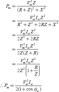
Now Voc is the open-circuit voltage, i.e., Vr when Ir = 0.
Let x be the distance from the sending end and l be the length of the line
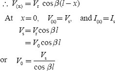
For a lossless line, r = 0 and g = 0, then the voltage at distance x from the sending end becomes
V(x) = Vr cos β(l − x) + jZcIr sin β(l − x)
where β is the phase constant
Suppose the line is open circuited at the receiving end, i.e., Ir = 0,
Similarly, the short-circuit current Isc is the value of Ir when Vr = 0

Assuming the line to be lossless, cos ϕsc = 0
Equation (9.43) represents loci of maximum power for different line lengths at unity p.f.
The receiving-end current, ![]()
The sending-end voltage of the line, if assuming the line to be lossless, now becomes
For a fixed sending-end voltage Vs and the fixed line length, Equation (9.44) is quadratic in Vr and thus will have two roots. Figure 9.25 shows a graphical relation between ![]() as a function of normalized loading
as a function of normalized loading ![]() .
.
From Fig. 9.25, it is observed that the maximum power can be transmitted for each load p.f. and for any loading, there are two different values of Vr.
The normal operation of the power system is along the upper part of the curve where the receiving-end voltage is nearly 1.0 p.u. The load is increased by decreasing the effective resistance of the load upto the maximum power; the product of load voltage and current increases as the system is stable. As the point of maximum power is reached, a further reduction in effective load resistance reduces the voltage more than the increase in current and therefore, there is an effective reduction in power transmission. The voltage finally collapses to zero and the system at the receiving end is effectively short-circuited and therefore, the power transmitted is zero (point at orgin in Fig. 9.25).
It is observed from Fig. 9.25 that the power transmitted is zero both at Point K and Point 0. Point K corresponding to the open circuit and Point 0 corresponding to the short circuit and in either case the power transmitted is zero.
Figure 9.25 shows the relation between ![]() as a function of normalized loading
as a function of normalized loading ![]() , where Pc is the surge impedance load. These relation curves between
, where Pc is the surge impedance load. These relation curves between ![]() and
and ![]() are known as normalized P–V curves. These P–V curves are different for different p.f.’s. At more leading p.f.’s, the maximum power is higher and for that the shunt compensation is provided. The nose voltage of the P–V curve has the critical voltage at the receiving end for maximum power transfer. With leading p.f., the critical voltage is higher, which is a very important aspect of voltage stability.
are known as normalized P–V curves. These P–V curves are different for different p.f.’s. At more leading p.f.’s, the maximum power is higher and for that the shunt compensation is provided. The nose voltage of the P–V curve has the critical voltage at the receiving end for maximum power transfer. With leading p.f., the critical voltage is higher, which is a very important aspect of voltage stability.
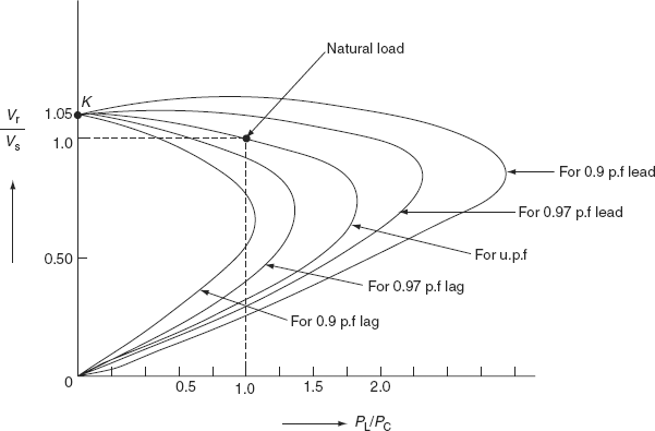
FIG. 9.25 ![]() as a function of normalized loading
as a function of normalized loading ![]()
The main disadvantage of the load-flow solution for P–V curves is that it is likely to diverge near the maximum power-transfer point or the nose point of the P–V curve. A load-flow solution is at various P–V buses or generators buses for particular generations. However, when the load changes, the scheduling of generation at various generator buses also changes. This is yet another disadvantage of the load-flow solution method.
9.18.2 Concept of voltage collapse proximate indicator
Consider that a purely inductive load is connected to a source through a lossless line as shown in Fig. 9.26.
Here, P = 0 and δ = 0 since the load is purely inductive; therefore, the reactive power at the receiving end is expressed as ![]() .
.
The condition for maximum reactive power transfer is ![]() .
.
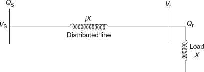
FIG. 9.26 Radial line connected with purely inductive load to source
where Vcritical is the receiving-end voltage for maximum reactive power transfer.
Therefore, the maximum reactive power is expressed as
As half of the drop will be across the line and another half across the load, Xload = X; hence, ![]() i.e., the maximum reactive power is transferred when the load reactance is equal to the line reactance or the source reactance.
i.e., the maximum reactive power is transferred when the load reactance is equal to the line reactance or the source reactance.
The short-circuit reactive power of the line is ![]() ; hence, the normalized maximum reactive power is
; hence, the normalized maximum reactive power is
![]()
Also ![]()
Now Qs = Qr + I2X
Since ![]()
Hence,
Multiplying both sides of Equation (9.45) by ![]() , we get
, we get

Now
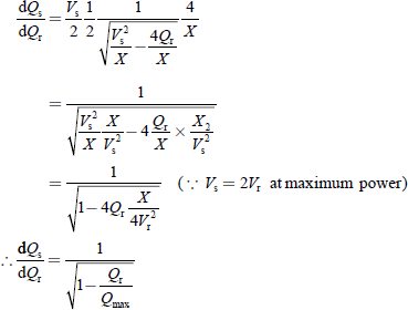
The differentiation of the sending-end reactive power Qs with respect to the receiving-end reactive power Qr, i.e., ![]() , is known as the voltage collapse proximate indicator (VCPI) of a radial line.
, is known as the voltage collapse proximate indicator (VCPI) of a radial line.
The receiving-end voltage varies from Vs at no load to ![]() at maximum load Qmax. However, VCPI is unity at no load since at no load Qr = 0 and
at maximum load Qmax. However, VCPI is unity at no load since at no load Qr = 0 and 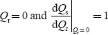 and it is infinity at maximum load since at this load Qr = Qr max and hence
 ![]()
It is clear that near the maximum load, an extremely large amount of reactive power is required at the sending end to supply an incremental increase in load. Thus, VCPI is a very sensitive indicator of impeding voltage collapse. There, lated quantities reactive reserve activation and reactive losses are also sensitive indicators.
9.18.3 Voltage-stability analysis: Q–V curves
Q–V curves can be obtained from the normalized P–V curves.
Let ![]()
For constant values of p, we note the two pairs of values of v and q for each p.f. and report these values. The result of these plots is shown in Fig. 9.27.

FIG. 9.27 Normalized Q–V curves for fixed source and reactive network loads are at constant power
The critical voltage is high for loadings (i.e., v is above 1 p.u. for p = 1 p.u.). The right-hand side of the curves indicates the normal operating conditions where the application of shunt capacitors raises the voltage. The steep-sloped linear portions of the right side of the curve are equivalent to the figure below (rotate Fig. 9.28 clock-wise by 90°).

FIG. 9.28 System approximate voltage-reactive power characteristic
The Q–V curves for large systems are obtained by a series of power-flow simulations. Q–V curves result from the plot of voltage at a test or critical bus versus reactive power on the same bus. Generally, the P–V bus or generator bus has reactive power constraints for a load-flow solution. A fictitious synchronous condenser is represented at the test bus and allows the bus to have any reactive power for a fixed p and v. The value of v at the bus changes for obtaining another point on the Q–V curve, and obtains reactive power flow for different scheduled voltages at the bus. Scheduled voltage at the bus is an independent variable and forms an abscissa variable. The capacitive reactive power required to maintain the scheduled voltage at the bus is a dependent variable and is plotted in the positive vertical direction. Without the application of shunt reactive compensation at the test bus, the operating point is at the zero reactive point corresponding to the removal of the fictitious synchronous condenser.
9.19 DERIVATION FOR VOLTAGE-STABILITY INDEX
Consider a typical branch consisting of sending- and receiving-end buses as shown in Fig. 9.29.
Current flowing through the branch,

The real term of the above equation is
VSVR cos(δ1 − δ2) = VR2 + (RP + XQ)
and the imaginary part is
VSVR sin(δ1 − δ2) = XP − RQ
Squaring and adding the above two terms, we get


FIG. 9.29 Single-line model of typical branch
The above equation is a quadratic equation of VR2. The system is to be stable if VR2 ≥ 0.
It is possible when
b2 − 4ac ≥ 0
i.e., [2(RP + XQ)− VS2)]2 − 4(P2 + Q2)(R2 + X2) ≥ 0
or 4R2p2 +4X2Q2 + 4R × PQ + VS4 − 4VS2 (RP + XQ)
− 4R2p2 − 4X2p2 − 4R2Q2 − 4X2Q2 ≥ 0
Simplifying the above equation, we get
VS4 − 4VS2 (RP − XQ) − 4(PX − RQ)2 ≥ 0
or 4(PX − RQ)2 + 4VS2 (RP + XQ) ≤ VS4
Dividing both sides of the above equation by VS4, we get

where L = stability index
For stable systems, L ≤ 1.
Example 9.1: A 440 V, 3-ϕ distribution feeder has a load of 100 kW at lagging p.f. with the load current of 200 A. If the p.f. is to be improved, determine the following:
- uncorrected p.f. and reactive load and
- new corrected p.f. after installing a shunt capacitor of 75 kVAr.
Solution:
- Uncorrected p.f.

- Corrected p.f.
Example 9.2: A synchronous motor having a power consumption of 50 kW is connected in parallel with a load of 200 kW having a lagging p.f. of 0.8. If the combined load has a p.f. of 0.9, what is the value of leading reactive kVA supplied by the motor and at what p.f. is it working?
Solution:
Let:
p.f. angle of motor = ϕ1
p.f. angle of load = ϕ2 = cos–1 (0.8) = 36.87°
Combined p.f. angle (both motor and load), ϕ = cos–1(0.9) = 25.84°
tan ϕ2 = tan 36° 87′ = 0.75; tan ϕ = tan 25°84′ = 0.4842
Combined power, P = 200 + 50 = 250 kW
Total kVAr of a combined system = P tan ϕ1 = 250 × 0.4842 = 121.05
Load kVAr = 200 × tan ϕ2 = 200 × 0.75 = 150
∴ Leading kVAr supplied by synchronous motor = 150 – 121.05 = 28.95
p.f. angle at which the motor is working, ϕ1 = tan–1 28.95/50 = 30.07°
p.f. at which the motor is working = cos ϕ1 = 0.865 (lead)
Example 9.3: A 3-ϕ, 5-kW induction motor has a p.f. of 0.85 lagging. A bank of capacitor is connected in delta across the supply terminal and p.f. raised to 0.95 lagging. Determine the kVAr rating of the capacitor in each phase.
Solution:
The active power of the induction motor, P = 5 kW
When the p.f. is changed from 0.85 lag to 0.95 lag by connecting a condenser bank, the leading kVAr taken by the condenser bank = P (tan ϕ2 – tan ϕ1)
= 5(0.6197 – 0.3287) = 1.455
∴ Rating of capacitor connected in each phase = 1.455/3 = 0.485 kVAr
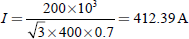
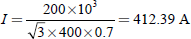
Example 9.4: A 400 V, 50 Hz, 3-ϕ supply delivers 200 kW at 0.7 p.f. lagging. It is desired to bring the line p.f. to 0.9 by installing shunt capacitors (Fig. 9.30). Calculate the capacitance if they are: (a) star connected and (b) delta connected.
Solution:
- For star connection:
Phase voltage, Vph = 400/
 = 230.94 V/ph
Load current,
The active component of current, Ia = I cos ϕ1 = 412.39 × 0.7 = 288.68 A
Reactive component of current,
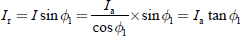
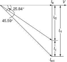
FIG. 9.30 Phasor diagram
For a fixed load, let us take:
The reactive component of load current without capacitor = Ia tan ϕ1
The reactive component of load current with capacitor = Ia tan ϕ2
Current taken by the capacitor installed for improving p.f., IC = Ia (tan ϕ1 – tanϕ2)
= 288.68 (tan (cos−1 0.7) − tan (cos−1 0.9))
= 154.7 A
The value of capacitor to be connected,


- For delta connection:
Phase voltage, Vph = 400 V
Load current,
Phase current,

The active component of phase current, Ia = I cos ϕ1 = 238.09 × 0.7 = 166.663 A
Current taken by the capacitor installed for improving p.f., IC = Ia (tanϕ1 – tanϕ2)
= 166.663 (tan (cos−1 0.7) − tan (cos−1 0.9))
= 89.312 A
The value of capacitor to be connected,

Example 9.5: A 3-ϕ 500 HP, 50 Hz, 11 kV star-connected induction motor has a full load efficiency of 85% at lagging p.f. of 0.75 and is connected to a feeder. If the p.f. of load is desired to be corrected to 0.9 lagging, determine the following:
- size of the capacitor bank in kVAr and
- capacitance of each unit if the capacitors are connected in Δ as well as in Y.
Solution:
Induction motor output = 500 HP
Efficiency η = 85%,
η = output/input
Input of the induction motor, P |
= |
output/η = 500/0.85 = 588.235 HP |
|
= |
588.235 × 746 = 438.82 kW |
Initial p.f. (cos ϕ1) |
= |
0.75 ⇒ tan ϕ1 = 0.88 |
Corrected p.f. (cos ϕ2) |
= |
0.9 ⇒ tan ϕ2 = 0.48 |
Leading kVAr taken by the capacitor bank, Qc |
= |
P (tan ϕ1 − tan ϕ2) |
|
= |
438.82 (0.88 − 0.48) = 175.53 kVAr |
Case 1: Delta connection:
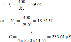
Charging current per phase, ![]()
Reactance of capacitor bank per phase,
![]()
Capacitance of capacitor bank,
Case 2: Star connection:
IL = Ic = 9.213 A
Reactance of capacitor bank per phase,
Capacitance of capacitor bank, ![]()
Example 9.6: A star-connected 400 HP (metric), 2, 000 V, and 50 Hz motor works at a p.f. of 0.7 lag. A bank of mesh-connected condensers is used to raise the p.f. to 0.9 lag. Calculate the capacitance of each unit and total number of units required, if each unit is rated 400 V, 50 Hz. The motor efficiency is 90% (Fig. 9.31).
Solution:
|
Motor output |
= 400 HP |
|
Supply voltage |
= 2, 000 V |
|
i.e., V |
= 2, 000 V |
|
p.f. without condenser |
= 0.7 lag |

FIG. 9.31 Circuit diagram
Efficiency of motor, η = 0.9;
For fixed loads, the active component of current is the same for improved p.f., whereas the reactive component will be changed.
∴ The active component of current at 0.7 p.f. lag., Ia1 = I cos ϕ1
=136.73 × 0.7 = 95.71 A
Line current taken by the capacitor installed for improving p.f., IC = Ia (tanϕ1 − tanϕ2)
= 95.71 (tan(cos−1 0.7)− tan(cos−1 0.9))
= 51.28 A
The bank of condensers used to improve the p.f. is connected in delta. The voltage across each phase is 2, 000 V, but each unit of condenser bank is of 400 V. So, each phase of the bank will have five condensers connected in series as shown in Fig. 9.31.
The current in each phase of the bank ![]()
Let Xc be the reactance of each condenser.
Then the charge current,
Capacitance of each phase of the bank ![]()
Example 9.7: A 3-ϕ, 50 Hz, 2,500 V motor develops 600 HP, the p.f. being 0.8 lagging and the efficiency 0.9. A capacitor bank is connected in delta across the supply terminals and the p.f. is raised to unity. Each of the capacitance units is built of five similar 500 V capacitors (Fig. 9.32). Determine the capacitance of each capacitor.

FIG. 9.32 Circuit diagram
Solution:
Motor input

Leading kVAr supplied by the capacitor bank = P(tan ϕ1 − tan ϕ2)
= 497.33 (0.75 − 0)
= 373 kVAr
Leading kVAr supplied by each of three sets

Current per phase of capacitor bank,
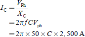
kVAr required/phase
But leading kVAr supplied by each phase = 124.33 kVAr
Since it is the combined capacitance of five equal capacitors joined in series,
The capacitance of each unit |
= 5 × 63.32 µF |
|
= 3,116.6 µF |
Example 9.8: A 3-ϕ, 50 Hz, 30-km transmission line supplies a load of 5 MW at p.f. 0.7 lagging to the receiving end where the voltage is maintained constant at 11 kV. The line resistance and inductance are 0.02 Ω and 0.84 mH per phase per km, respectively. A capacitor is connected across the load to raise the p.f. to 0.9 lagging (Fig. 9.33). Calculate: (a) the value of the capacitance per phase and (b) the voltage regulation.
Solution:
Length of the line |
= 30 km |
Frequency |
= 50 Hz |
Load |
= 5 MW at 0.7 lagging p.f. |
Receiving-end voltage, Vr |
= 11 kV |
Line resistance per phase = 0.02 Ω per km |
= 0.02 × 30 = 0.6 Ω |
Reactance of 30-km length per phase, X |
= 2 × π × f × L × 30 |
|
= 2 × π × 50 × 0.84 × 10–3 × 30 = 7.92 Ω |

FIG. 9.33 Phasor diagram
For fixed loads, the active component of power is the same for improved p.f., whereas the reactive component of power will be changed.
∴ The active component of current at 0.7 p.f. lag, P = 5 MW
Reactive power (MVAr) supplied by the capacitor bank = P(tan ϕ1 − tan ϕ2)
= 5 (1.02 − 0.484)
= 2.679 MVAr
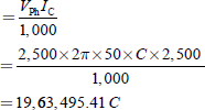
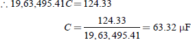
Reactive power (MVAr) supplied by the capacitor bank = ![]()
Let C be the capacitance to be connected per phase across the load.
kVAr required/phase

But leading kVAr supplied by each phase = 893 kVAr

Sending-end voltage with improved p.f. = Vr + I(R cos ϕ2 + jX sin ϕ2)
Receiving-end voltage,
Current with improved p.f.,
∴ Sending-end voltage, Vs |
= 6,350.85 + 291.59(0.6 × 0.9 + j 7.92 × 0.436) |
|
= 6,508.31 + j1006.9 V/ph |
|
= 6,585.74∠8.79 V/ph |
|
= 11, 406.84 V(L-L) |
Example 9.9: A synchronous motor improves the p.f. of a load of 200 kW from 0.7 lagging to 0.9 lagging and at the same time carries an additional load of 100 kW (Fig. 9.34). Find: (i) The leading kVAr supplied by the motor, (ii) kVA rating of motor, and (iii) p.f. at which the motor operates.
Solution:
Load, P1 |
= 200 kW |
Motor load, P2 |
= 100 kW |
p.f. of the load 200 kW |
= 0.7 lag |
p.f. of the combined load (200 + 100) kW |
= 0.9 lag |
Combined load |
= P1 + P2 = 200 + 100 = 300 kW |
∆OAB is a power triangle without additional load, ∆ODC the power triangle for combined load, and ∆BEC for the motor load.
From Fig. 9.34, we have
(i) Leading kVAr taken by the motor |
= |
CE |
|
= |
DE – DC = AB – DC |
|
= |
200 tan(cos–10.7) – 300 tan(cos–10.9) |
|
= |
200 × 1.02 – 300 × 0.4843 |
|
= |
58.71 KVAr |
(ii) kVA rating of motor |
= BE |
|
|
|
|
|
= 115.96 kVA |

FIG. 9.34 Phasor diagram
|
|
|
|
|
= 0.862 leading |
Example 9.10: A 37.3 kW induction motor has p.f. 0.9 and efficiency 0.9 at full-load, p.f. 0.6, and efficiency 0.7 at half-load. At no-load, the current is 25% of the full-load current and p.f. 0.1. Capacitors are supplied to make the line p.f. 0.8 at half-load. With these capacitors in circuit, find the line p.f. at (i) full-load and (ii) no-load.
Solution:
Full-load current, I1 = 37.3 × 10³/(![]() VL × 0.9 × 0.9) = 26,586/VL
VL × 0.9 × 0.9) = 26,586/VL
At full load:
Motor input, P1 = 37.3/0.9 = 41.44 kW
Lagging kVAr drawn by the motor, kVAr1 = P1 tan ϕ1 = 41.44 tan(cos–1 0.9) = 20.07
At half load:
Motor input, P2 = (0.5 × 37.3)/0.7 = 26.64 kW
Lagging kVAr drawn by the motor, kVAr2 = P2 tan ϕ2 = 26.64 tan(cos–1 0.6) = 35.52
At no load:
No-load current, I0 = 0.25 (full-load current) = 0.25 × 26,586/VL = 6,646.5/VL
Motor input at no-load, Po = ![]() VLI0 cos ϕ0
VLI0 cos ϕ0
= ![]() × 6,646.5 × VL × 0.1/VL = 1.151 kW
× 6,646.5 × VL × 0.1/VL = 1.151 kW
Lagging kVAr drawn by the motor, kVAr0 = 1.151 tan(cos–1 0.1)
= 11.452
Lagging kVAr drawn from the mains at half-load with capacitors,
kVAr supplied by capacitors, kVArc = kVAr2 – kVAr2c = 35.52 – 19.98 = 15.54
kVAr drawn from the main at full load with capacitors kVAr1c = kVAr1 – kVArc
- Line p.f. at full load

- kVAr drawn from mains at no-load with capacitors = 11.452 – 15.54 = – 4.088
Line p.f. at no-load = cos (tan–1 – 4.088/1.151) = cos (–74.27°) = 0.271 leading.
Example 9.11: A single-phase system supplies the following loads:
- Lighting load of 50 kW at unity p.f.
- Induction motor load of 125 kW at p.f. 0.707 lagging.
- Synchronous motor load of 75 kW at p.f. 0.9 leading.
- Other miscellaneous loads of 25 kW at p.f. 0.8 lagging.
Determine the total kW and kVA delivered by the system and the p.f. at which it works.
Solution:
Total kW of the load |
= |
50 + 125 + 75 + 25 = 275 kW |
kVAr of lighting load |
= |
50 × 0 = 0 |
kVAr of induction motor |
= |
−125 tan(cos−1 0.707) = −125.04 |
kVAr of synchronous motor |
= |
75 tan(cos−1 0.9) = 36.32 |
kVAr of miscellaneous loads |
= |
25 tan(cos−1 0.8) = −18.75 |
∴ Total kVAr of the load |
= |
0 − 125.04 + 36.32 − 18.75 = −107.47 |

KEY NOTES
- For quality power, i.e., voltage and frequency at every supply point would remain constant, free from harmonics, and the power factor would remain unity, compensation is required.
- The objectives of load compensation are:
- Power-factor correction.
- Voltage regulation improvement.
- Balancing of load.
- Characteristics of the ideal compensator are to:
- Provide a controllable and variable amount of reactive power without any delay according to the requirements of the load.
- Maintain constant-voltage characteristics at its terminals.
- Operate independently in the three phases.
- Voltage regulation is defined as the proportional change in supply-voltage magnitude associated with a defined change in load current, i.e., from no-load to full load.
- The SIL of a transmission line is the MW loading of a transmission line at which a natural reactive power balance occurs (zero resistance).
- Voltage stability: A power system at a given operating state and subjected to a given disturbance is voltage stable if voltages near loads approach post-disturbance equilibrium values. The disturbed state is within the regions of attractions of stable post-disturbance equilibrium.
- Voltage collapse: Following voltage instability, a power system undergoes voltage collapse if the post-disturbance equilibrium voltages near the load are below the acceptable limits. The voltage collapse may be either total or partial.
SHORT QUESTIONS AND ANSWERS
- Define the need of compensation.
For maintaining the quality power, i.e., voltage and frequency at every supply point would remain constant, free from harmonics and the p.f. would remain unity and compensation is needed.
- What are the objectives of load compensation?
The objectives of load compensation are:
- p.f. correction.
- Voltage regulation improvement.
- Balancing of load.
- What are the characteristics of an ideal compensator?
The characteristics of the ideal compensator are:
- To provide a controllable and variable amount of reactive power without any delay according to the requirements of the load.
- To maintain a constant-voltage characteristic at its terminals and
- Should operate independently in the three phases.
- Define the voltage regulation.
It is defined as the proportional change in supply voltage magnitude associated with a defined change in load current, i.e., from no load to full load.
- Define the surge impedance loading (SIL) of a transmission line.
It is the MW loading of a transmission line at which a natural reactive power balance occurs (zero resistance).
- What is meant by voltage stability?
A power system at a given operating state and subjected to a given disturbance is voltage stable if voltages near loads approach post-disturbance equilibrium values. The disturbed state is within the regions of attractions of stable post-disturbance equilibrium.
- What is meant by voltage collapse?
Following voltage instability, a power system undergoes voltage collapse if the post-disturbance equilibrium voltages near the load are below acceptable limits. The voltage collapse may be either total or partial.
MULTIPLE-CHOICE QUESTIONS
- The major reason for low lagging p.f. of supply system is due to the use of __________ motors.
- Induction.
- Synchronous.
- DC.
- None of these.
- The maximum value of p.f. can be __________.
- 1.
- 0.9.
- 0.8.
- 0.7.
- By improving the p.f. of the system, the kilowatts delivered by generating stations are __________.
- Decreased.
- Increased.
- Not changed.
- None of these.
- Power factor can be improved by installing such a device in parallel with load, which takes:
- Lagging reactive power.
- Leading reactive power.
- Apparent power.
- None of these.
- The main reason for low p.f. of supply system is due to the use of __________.
- Resistive load.
- Inductive load.
- Synchronous motor.
- All of these.
- The only motor that can also be worked at leading p.f. and can supply mechanical power __________.
- Synchronous induction generator.
- Synchronous motor.
- Alternator.
- None of these.
- An over-excited synchronous motor on no-load is known as __________.
- Synchronous induction generator.
- Synchronous condenser.
- Alternator.
- None of these.
- For synchronous condensers, the p.f. improvement apparatus should be located at __________.
- Sending end.
- Receiving end.
- Both (a) and (b).
- None of these.
- A disadvantage of synchronous condenser is:
- Continuous losses in motor.
- High maintenance cost.
- Noisy.
- All of the above.
- The smaller the lagging reactive power drawn by a circuit, its p.f. will be __________.
- Better.
- Poorer.
- Unity.
- None of these.
- kVAR is equal to __________.
- kW tan ϕ.
- kW sin ϕ.
- kVA cos ϕ.
- None of these.
- For a particular power, the current drawn by the circuit is minimum when the value of p.f. is __________.
- 0.8 lagging.
- 0.8 leading.
- Unity.
- None of these.
- Synchronous capacitors are normally ____________ cooled.
- Air.
- Oil.
- Water.
- None of these.
- To improve the p.f. of 3-ϕ circuits, the size of each capacitor when connected in delta with respect to when connected in star is __________.
- 1/6th.
- 1/4th.
- 3 times.
- 1/3rd.
- The p.f. improvement equipment is always placed __________.
- At the generating station.
- Near the transformer.
- Near the apparatus responsible for low p.f.
- Near the bus bar.
- A synchronous machine has higher capacity for:
- Leading p.f.
- Lagging p.f.
- It does not depend upon the p.f. of the machine.
- None of these.
- If a synchronous machine is underexcited, it takes lagging VARs from the system when it is operated as a __________.
- Synchronous motor.
- Synchronous generator.
- Synchronous motor as well as generator.
- None of these.
- A synchronous phase modifier as compared to synchronous motor used for mechanical loads has __________.
- Larger shaft and higher speed.
- Smaller shaft and higher speed.
- Larger shaft and smaller speed.
- Smaller shaft and smaller speed.
- The phase advancer is mounted on the main motor shaft and is connected in the __________ motor.
- Rotor.
- Stator.
- Core.
- None of these.
- Industrial heating furnaces such as arc and induction furnaces operate on __________.
- Very low lagging p.f.
- Very low leading p.f.
- Very high leading p.f.
- None of these.
- If a synchronous machine is overexcited, it takes lagging VARs from the system when it is operated as:
- Synchronous motor.
- Synchronous generator.
- Synchronous motor as well as generator.
- None of these.
- A machine designed to operate at full load is physically heavier and is costlier if the operating p.f. is:
- Lagging.
- Leading.
- The size and cost do not depend on p.f.
- None of these.
- Unit of reactive power is:
- MW.
- MVAr.
- MVA.
- KVA.
- Reactive power is ____________ power.
- Wattfull.
- Wattless.
- Loss.
- None of these.
- Transmission line parameters are:
- R.
- L.
- C.
- All of these.
- On fundamental Tγ. line expression V(x) = Aeγ x + Be-γ x, γ represents:
- Distance (or) length.
- Velocity of light.
- Propagation constant.
- None of these.
- Characteristic impedance is _____________.
- β is ____________.


- All of these.
- Advantage of operating at natural load is:
- Insulation is uniformly stressed.
- Reactive power balance is achieved.
- Both (a) and (b).
- None of these.
- An uncompensated line on open-circuit leads to __________.
- Ferranti effect.
- line-charging current flowing into generators is more.
- Both (a) and (b).
- None of these.
- A symmetrical line at no-load means __________.
- No power transmission.
- Vs = Vr.
- Both (a) and (b).
- None of these.
- During the underexcited operation of a synchronous generator:
- Heating of the ends of the stator core increases.
- Reduces field current, results in the internal emf, which causes weak stability.
- Both (a) and (b).
- None of these.
- For a symmetrical line with Vs = V0, the maximum voltage occurs at:
- Sending end.
- Receiving end.
- Midpoint.
- None of these.
- Unit of p.f. is:
- s.
- m.
- No units.
- None of these.
- Unit of time constant is:
- m.
- kg.
- s.
- miles.
- Power transmission through a line is improved by:
- Increasing the line voltage.
- Decreasing the line reactance.
- Both (a) and (b).
- None of these.
- A linear device must satisfy:
- Homogeneity.
- Additivity.
- Both (a) and (b).
- None of these.
- Fundamental requirements of AC-power transmission is:
- Synchronous machines must remain stably in synchronizer.
- Voltages must be kept near to their rated values.
- Both (a) and (b).
- None of these.
- Load compensation is:
- The control of reactive power to improve quality of supply.
- The control of real power to improve quality of supply.
- The control of voltage and its angle to improve the quality of supply.
- Both (a) and (b).
- Power factor under natural load is:
- Lagging.
- Leading.
- Unity.
- None of these.
- Steady-state stability of unit occurs when δ = __________.
- 30°.
- 20°.
- 90°.
- 0°.
- ‘θ’ in fundamental transmission line equation is:
- β.
- ax.
- βl.
- β/a.
- Rating of a compensator is:
- MVAr.
- Time of response.
- Both (a) and (b).
- None of these.
- Load compensation includes:
- p.f. correction.
- Voltage regulation.
- Load balancing.
- All of these.
- For a symmetrical line, the voltage is more at:
- Sending end.
- Receiving end.
- Midpoint.
- All of these.
- Load compensation can be achieved by:
- Installing the compensating equipment near the source.
- Installing the compensating equipment near the load.
- Either (a) or (b).
- Both (a) and (b).
- pf correction of load is achieved by:
- Generating reactive power as close as possible to the source.
- Generating reactive power as close as possible to the load.
- Generating real power as close as possible to the load.
- Generating real power as close as possible to the source.
- The main function of an ideal compensator is:
- Instantaneous pf correction to unity.
- Elimination (or) reduction of voltage regulation.
- Phase balance of the load currents and voltages.
- All.
- The important characteristic of an ideal compensator is:
- To provide a controllable and variable amount of reactive power without any delay.
- To maintain a constant voltage characteristic at its terminals.
- Should operate independently in the three phases.
- All the above.
- Characteristic impedance of the line depends upon:
- The characteristic of the line per unit length.
- Length of the line.
- Radius and spacing between conductors.
- All.
- The surge impedance loading (SIL) is expressed as:

- SIL = (VL-L)2 × surge impedance.
- None.
- When a line is loaded above its SIL, it acts like:
- Shunt reactor absorbing MUAR from the system.
- Shunt capacitor supplying MUAR to the system.
- Series capacitor supplying MUAR to the system.
- Series reactor absorbing MUAR from the system.
- When a line is loaded below its SIL, it acts like:
- Shunt reactor absorbing MUAR from the system.
- Shunt capacitor supplying MUAR to the system.
- Shunt capacitor supplying MUAR to the system.
- Shunt reactor absorbing MUAR from the system.
- If any inductive load is connected at the sending end of the line, it will support the synchronous generators:
- To absorb the line-charging reactive power.
- To absorb the load-charging reactive power.
- To supply the line-charging reactive power.
- To supply the load-charging reactive power.
- The change in electrical properties of a transmission line in order to increase its power transmission capability is known as:
- Load compensation.
- Line compensation.
- Load synchronism.
- Line synchronism.
- Apply series capacitors to reduce XL and thereby reduce θ at the fundamental frequency. This method is called:
- Line-length compensation (or) θ-compensation.
- Compensation by sectioning.
- Load balancing.
- All the above.
- Series compensation results in:
- Increase in maximum transferable power capacity.
- Decrease in transmission angle for considerable amount of power transfer.
- Increase in virtual surge impedance loading.
- All the above.
- For a heavy loading condition, a flat voltage profile can be obtained by:
- Series compensation.
- Shunt compensation.
- (a) or (c).
- None.
- Inductive shunt compensation __________ the virtual surge impedance and __________ the virtual SIL of the line:
- Decreases, decreases.
- Decreases, increases.
- Increases, decreases.
- Decreases, increases.
- If the inductive shunt compensation is 100% then:
- Flat voltage profile exists at zero loads.
- Ferranti effect can be eliminated.
- Both (a) and (b).
- None.
- Sub-synchronous resonance (SSR) is treated as __________ type of phenomenon.
- Electrical.
- Mechanical.
- Combined electrical–mechanical.
- Damped frequency resonance.
- UPFC is able to perform:
- Voltage support.
- Power flow control.
- Improved stability.
- All.
- The voltage stability analysis is carried out by which power flow-based method?
- P–V curves.
- Q–V curves.
- Both (a) and (b).
- None.
- Voltage collapse proximate indicator (VCPI) for a radial line is defined as:
REVIEW QUESTIONS
- Explain the objectives of load compensation.
- Explain the voltage regulation with and without compensators.
- What are the specifications of load compensation?
- Explain the effects on uncompensated line under no-load and load conditions.
- Explain the effects on compensated line.
- Explain the concept of sub-synchronous resonance.
- Compare the different types of compensating equipment for transmission systems.
- Explain the concepts of voltage stability and voltage collapse.
- Derive the voltage stability index of a typical branch of a power system.
PROBLEMS
- A 3-ϕ, 5 kW induction motor has a p.f. of 0.8 lag. A bank of capacitors is connected in delta across the supply terminals and p.f. is raised to 0.95 lag. Determine the kVAr rating of the capacitors connected in each phase.
- A 3-ϕ, 50 Hz, 400 V motor develops 100 HP, the p.f. being 0.7 lag and efficiency 93%. A bank of capacitors is connected in delta across the supply terminals and p.f. is raised to 0.95 lag. Each of the capacitance units is built of four similar 100 V capacitors. Determine the capacitance of each capacitor.
- A star-connected 400 HP, 2,000 V, 50 Hz motor works at a p.f. of 0.75 lagging. A bank of mesh-connected condensers is used to raise the p.f. to 0.98 lagging. Determine the capacitance of each unit and total number of units required; if each is rated 500 V, 50 Hz. The motor efficiency is 85%.
- A 3-ϕ, 50 Hz, 3,000 V motor develops 600 HP, the p.f. being 0.75 lagging and the efficiency 0.95. A bank of capacitors is connected in delta across the supply terminals and the p.f. raised to 0.98 lagging. Each of the capacitance units is built of five similar 600 V capacitors. Determine the capacitance of each capacitor.