
3
Economic Load Dispatch-II
OBJECTIVES
After reading this chapter, you should be able to:
- develop the mathematical model for economical load dispatch when losses are considered
- derive transmission loss expression
- study the optimal allocation of total load among the units
- develop a flowchart for the solution of optimization problem
3.1 INTRODUCTION
In case of an urban area where the load density is very high and the transmission distances are very small, the transmission loss could be neglected and the optimum strategy of generation could be based on the equal incremental production cost. If the energy is to be transported over relatively larger distances with low load density, the transmission losses, in some cases, may amount to about 20–30% of the total load; hence, it is essential to take these losses into account when formulating an economic load dispatch problem.
3.2 OPTIMAL GENERATION SCHEDULING PROBLEM: CONSIDERATION OF TRANSMISSION LOSSES
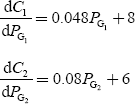
In a practical system, a large amount of power is being transmitted through the transmission network, which causes power losses in the network (PL) as shown in Fig. 3.1.
In finding an optimal solution for economic scheduling problem (allocation of total load among the generating units), it is more realistic to consider the transmission line losses, which are about 5–15% of the total generation.
In general, the condition for optimality, when losses are considered, is different. Equal incremental fuel costs (IFCs) for all generating units will not give an optimal solution.
3.2.1 Mathematical modeling
Consider the objective function:
Minimize Equation (3.1) subject to the following equality and inequality constraints:
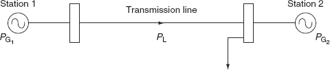
FIG. 3.1 Transmission network
(i) Equality constraint
The real-power balance equation, i.e., total real-power generations minus the total losses should be equal to the real-power demand:
i.e.,
(or)
where PL is the total transmission losses (MW), PD the total real-power demand (MW), and pGi the real-power generation at the ith unit (MW).
(ii) Inequality constraints
Always there will be upper and lower limits for real and reactive-power generation at each of the stations. The inequality constraints are represented:
- In terms of real-power generation as
PGi (min) ≤ PGi ≤ PGi (max) (3.3)
- In terms of reactive-power generation as
QGi (min) ≤ QGi ≤ QGi (max) (3.4)
The reactive-power constraints are to be considered since the transmission line results in loss is a function of real and reactive-power generations and also the voltage at the station bus.
- In addition, the voltage at each of the stations should be maintained within certain limits:
i.e., Vi (min) ≤ Vi ≤ Vi (max) (3.5)
The optimal solution should be obtained by minimizing the cost function satisfying constraint Equations (3.2) – (3.5).
3.3 TRANSMISSION LOSS EXPRESSION IN TERMS OF REAL-POWER GENERATION–DERIVATION
Transmission loss PL is expressed without loss of accuracy as a function of real-power generations. The power loss is expressed using B-coefficients or loss coefficients.
The expression for transmission power loss is derived using Kron’s method of reducing a system to an equivalent system with a single hypothetical load.
The expression is based on several assumptions as follows:
- All the lines in the system have the same
 ratio.
 - All the load currents have the same phase angle.
- All the load currents maintain a constant ratio to the total current.
- The magnitude and phase angle of bus voltages at each station remain constant.
- Power factor at each station bus remains constant.
We will derive an expression for the power loss of a system, having two generating stations, supplying an arbitrary number of loads through a transmission network as shown in Fig. 3.2(a).
To determine the current in any line, say k th line, apply the superposition principle and determine the current passing through the line, Ik.
The current distribution factor of a transmission line w.r.t. a power source is the ratio of the current it would carry to the current that the source would carry when all other sources are rendered inactive, i.e., sources that are not supplying any current.
Let us assume that the entire load current is supplied by generating station-1 only as shown in Fig. 3.2(b).
Current in the kth line = Ik1
Current distribution factor, ![]()
If we assume that the entire load is supplied by the second generating station only as shown in Fig. 3.2(c):
The current flowing through the kth line = Ik1
Current distribution factor, ![]()

FIG. 3.2 (a) Transmission network with two generating stations; (b) load supplied by generating station-1 only; (c) load supplied by generating station-2 only; (d) load supplied by two generating stations simultaneously; (e) source currents with respect to reference; (f) current in kth line
Because of assumptions (i) and (ii), the current distribution factors will be real numbers rather than complex numbers.
And also assuming that the total load is being supplied by both the stations as shown in Fig. 3.2(d):
The current in the kth line = Ik
From the relations,
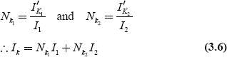
Although the current distribution factors are real numbers, the various source currents supplying total load will not be in phase, i.e., I1 and I2 are not in phase.
Let the source currents I1 and I2 be expressed as I1∠σ1 and I2∠σ2 as shown in Fig. 3.2(e).
Then, Ik = Nk1 I1 ∠σ1 + Nk2 I2 ∠σ2 with a phase difference of (σ2 – σ1) as shown in Fig. 3.2(f).
By adding Ik1 and Ik2 phasors, we have
The station currents are related as
and
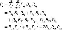
The power loss in the k th line can be calculated as 3 |Ik|2 Rk
i.e.,
power loss
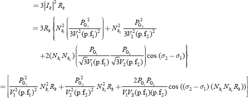
If there are ‘l ’ number of lines in the system, total power loss in the system can be calculated as
i.e.,

This above expression can be written as
where
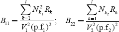
and
Equation (3.8) expresses the total loss as a function of real-power generations, PG1 and PG2.
The coefficients B11, B22, and B12 are called loss coefficients (or) B-coefficients and the unit is (MW)–1 and is also considered to be a constant in view of the assumptions made.
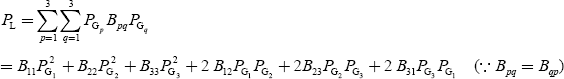
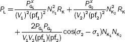
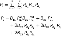
The same procedure can be extended for systems having more number of stations. If the system has ‘n’ number of stations, supplying the total load through transmission lines, the transmission line loss is given by
when n = 2,
Similarly for n = 3,
Since the transmission lines are symmetrical, loss coefficients Bpq and Bqp are equal, i.e., Bpq = Bqp.
The Bpq coefficients are loss coefficients and can be represented in matrix form of an n-generator system as
The diagonal elements of these coefficients are all positive and strong (since generating stations are interconnected) as compared with the off-diagonal elements, which mostly are negative and are relatively weaker.
These coefficients are determined for a large system by an elaborate digital computer program starting from the assembly of the open-circuit impedance matrix of the transmission line, which is quite lengthy and time-consuming. Besides, the formulations of B-coefficients are based on several assumptions and do not take into account the actual conditions of the system; the solution for the plant generations cannot be expected to be the best for minimum cost of generation.
3.4 MATHEMATICAL DETERMINATION OF OPTIMUM ALLOCATION OF TOTAL LOAD WHEN TRANSMISSION LOSSES ARE TAKEN INTO CONSIDERATION
Consider a power station having ‘n’ number of units. Let us assume that each unit does not violate the inequality constraints and let the transmission losses be considered.
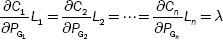
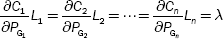
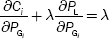
Assuming that the inequality constraint is satisfied, the objective function is redefined by augmenting Equation (3.1) with equality constraint (Equation (3.2)) using Lagrangian multiplier (λ) and is given by
This augmented objective function is called constrained objective function.
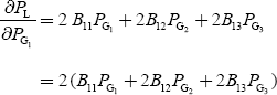
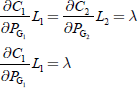
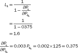
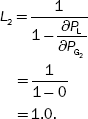
In the above objective function, the real-power generations are the control variables and the condition for optimality becomes ![]()
i.e.,

(or)


(or)
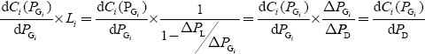
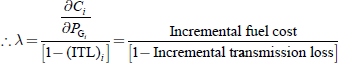
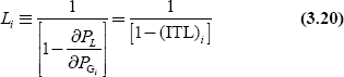
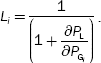
where ![]() represents the variation of total transmission loss with respect to real-power generation of the ith station and is called incremental transmission loss (ITL) of the ith station. Equation (3.14) can be written as
represents the variation of total transmission loss with respect to real-power generation of the ith station and is called incremental transmission loss (ITL) of the ith station. Equation (3.14) can be written as

or
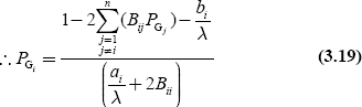
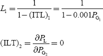
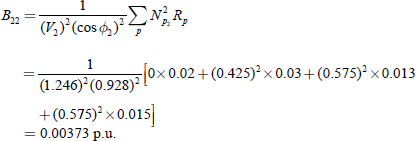
where  and is called the penalty factor of the ith station. Equation (3.15) can be utilized to obtain the optimal cost of operation.
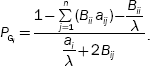
The condition for optimality when the transmission losses are considered is that the IFC of each plant multiplied by its penalty factor must be the same for all the plants:
i.e.,
Equation (3.12) is a set of n equations with (n + 1) unknowns. Here, the powers of n generators are unknown and λ is also unknown. These equations are known as exact co-ordination equations because they co-ordinate the ITL with IFC.
The following points should be kept in mind for the solution of economic load dispatch problems when transmission losses are included and co-ordinated:
- Although incremental production cost of a plant is always positive, ITL can either be positive or negative.
- The individual units will operate at different incremental production costs.
- The generation with the highest positive ITL will operate at the lowest incremental production cost.
For a small increase in received load by ΔPD, the ith plant generation is only changed by ∆PG1 and the generations of the remaining units are unaffected. Let ΔPL be the change in transmission loss, the power balance equation becomes ∆PGi − ∆ PL = ∆PD.
Thus,
when ![]() is the incremental cost of the received power of the ith plant and the penalty factor
is the incremental cost of the received power of the ith plant and the penalty factor ![]() . This means that as ∆PGi increment has a larger proportion dissipated as loss,
. This means that as ∆PGi increment has a larger proportion dissipated as loss, ![]() approaches unity and the penalty factor ‘Li’ increases without bound. Thus, for a larger penalty factor ‘Li’, unit ‘i ’ should be operated at low incremental cost implying a low power output.
approaches unity and the penalty factor ‘Li’ increases without bound. Thus, for a larger penalty factor ‘Li’, unit ‘i ’ should be operated at low incremental cost implying a low power output.
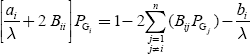
3.4.1 Determination of ITL formula
When a system consists of three generating units, i.e., n = 3, the transmission loss is
ITL of Generator-1 is obtained as
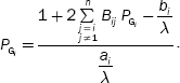
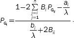
In general,
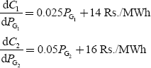
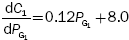
We know that the IFC of the ith unit is
Substitute Equations (3.17) and (3.18) in Equation (3.9); we get

Dividing the above equation by λ, we get
To solve this allocation problem, solve the co-ordination Equation (3.19) for a particular value of λ iteratively starting with an initial set of values of PGi (such as all PGi set to minimum values) and get the solution within a specified tolerance till all PGi’s converge, then check for power balance and if it is to be satisfied, then it is the optimal solution. If the power balance equation is not satisfied, modify the value of λ to a suitable value and solve the co-ordination equation.
3.4.2 Penalty factor
Consider Equation (3.12):

The above expression can be written as
or ![]()
where

is called the penalty factor of the ith station
The penalty factor of any unit is defined as the ratio of a small change in power at that unit to the small change in received power when only that unit supplies this small change in received power.
3.5 FLOWCHART FOR THE SOLUTION OF AN OPTIMIZATION PROBLEM WHEN TRANSMISSION LOSSES ARE CONSIDERED
When transmission losses are taken into account, the solution of an optimization problem is represented by the following flowchart (Fig. 3.3).
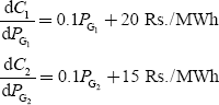
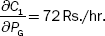
Example 3.1: The fuel cost functions in Rs./hr for two thermal plants are given by
where P1, P2 are in MW. Determine the optimal scheduling of generation if the total load is 640.82 MW. Estimate value of λ = 12 Rs./MWh. The transmission power loss is given by the expression
Solution:
%MATLAB PROGRAM FOR ECONOMIC LOAD DISPATCH WITH LOSSES AND NO GENERATOR
%LIMITS (dispatch3.m)
clc;
clear;
% uno d b a
costdata = [1 420 9.2 0.004;
2 350 8.5 0.0029];
ng = length(costdata(:,1));
for i = 1:ng
uno(i) = costdata(i,1);
d(i) = costdata(i,2);
b(i) = costdata(i,3);
a(i) = costdata(i,4);
end
lambda = 12;
pd = 640.82;
delp = 0.1;
dellambda = 0;
lossdata = [0.0346 0.00643];
totgencost = 0;
for i = 1:ng
B(i) = lossdata(1,i);
end
iter = 0;
disp(‘iter lambda pg1 pg2 ploss’);
while (abs(delp)> = 0.001)
iter = iter + 1;
lambda = lambda + dellambda;
pl = 0;
sum = 0;
delpla = 0;
for i = 1:ng
den = 2*(a(i) + lambda*B(i)*0.01);
p(i) = (lambda-b(i))/den;
pl = pl + (B(i)*0.01*p(i)*p(i));
sum = sum + p(i);
end
delp = pd + pl-sum;
for i = 1:ng
den = 2*(a(i) + lambda*B(i)*0.01)^2;
delpla = delpla + (a(i) + B(i)*0.01*b(i))/den;
end
dellambda = delp/delpla;
[iter;lambda;p(1);p(2);pl]’
end
for i = 1:ng
den = 1-(B(i)*p(i)*2*0.01);
l(i) = 1/den;
end
totgencost = 0;
for i = 1:ng
totgencost = totgencost + (d(i) + b(i)*p(i) + a(i)*p(i)*p(i));
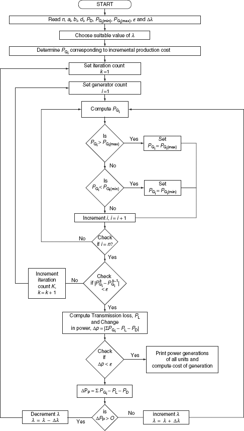
FIG. 3.3 Flowchart
ifc(i) = 2*a(i)*p(i) + b(i);
end
disp(‘FINAL OUTPUT OF MATLAB PROGRAM dispatch3.m’);
lambda
disp(‘GENERATING UNIT OPTIMALGENERATION(MW)’);
[uno; p]’
disp(‘INCREMENTAL FUEL COST AND PENALTY FACTORS ARE’);
disp(‘UNIT NO. IFC L’);
[uno;ifc;l]’
disp(‘CHECK LAMBDA = IFC*L’);
disp(‘UNIT NO. LAMBDA’);
[uno;ifc.*l]’
disp(‘TOTAL GENERATION COST(Rs./h)’);
totgencost
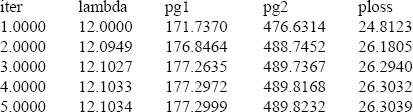
FINAL OUTPUT OF MATLAB PROGRAM dispatch3.m
lambda = 12.1034
GENERATING UNIT |
OPTIMAL GENERATION (MW) |
1.0000 |
177.2999 |
2.0000 |
489.8232 |
INCREMENTAL FUEL COSTS AND PENALTY FACTORS ARE:
UNIT NO. |
IFC |
L |
1.0000 |
10.6184 |
1.1398 |
2.0000 |
11.3410 |
1.0672 |
CHECK LAMBDA = IFC*L
UNIT NO. |
LAMBDA |
1.0000 |
12.1034 |
2.0000 |
12.1034 |
TOTAL GENERATION COST (Rs./hr) = 7386.20
Example 3.2: The fuel cost functions in Rs./hr for two thermal plants are given by
where P1, P2, P3 are in MW and plant outputs are subjected to the following limits. Determine the optimal scheduling of generation if the total load is 640.82 MW. Estimate the value of λ = 12 Rs./MWh.
Solution:
%MATLAB PROGRAM FOR ECONOMIC LOAD DISPATCH WITH LOSSES AND GENERATOR
%LIMITS(dispatch4.m)
clc;
clear;
% uno d b a pmin pmax
costdata = [1 420 9.20. 004 100 200;
2 350 8.5 0.0029 150 500];
ng = length(costdata(:,1));
for i = 1:ng
uno(i) = costdata(i,1);
d(i) = costdata(i,2);
b(i) = costdata(i,3);
a(i) = costdata(i,4);
pmin(i) = costdata(i,5);
pmax(i) = costdata(i,6);
end
lambda = 12;
pd = 640.82;
delp = 0.1;
dellambda = 0;
lossdata = [0.03460.00643];%NOTINPU
totgencost = 0;
for i = 1:ng
B(i) = lossdata(1, i);
end
whileabs(delp)> = 0.001
lambda = lambda + dellambda;
pl = 0;
sum = 0;
delpla = 0;
for i = 1:ng
den = 2*(a(i) + lambda*B(i)*0.01);
p(i) = (lambda-b(i))/den;
pl = pl + (B(i)*0.01*p(i)*p(i));
sum = sum + p(i);
end
delp = pd + pl-sum;
for i = 1:ng
den = 2*(a(i) + lambda*B(i)*0.01)^2;
delpla = delpla + (a(i) + B(i)*0.01*b(i))/den;
end
dellambda = delp/delpla;
end
dellambda = 0;
pv(i) = 0;
pvfi n(i) = 0;
end
limvio = 0;
for i = 1:ng
if p(i)<pmin(i)|p(i)> pmax(i)
limvio = 1;
break;
end
end
if limvio = =0
disp(‘GENERATION IS WITHIN THE LIMITS’);
end
delp = 0.1;
if limvio = =1
while (abs(delp)> = 0.01)
disp(‘GENERATION IS NOT WITHIN THE LIMITS’);
disp(‘VIOLATED GENERATOR NUMBER’);
i
if p(i)< pmin(i)
disp(‘GENERATION OF VIOLATED UNIT(MW)’);
p(i)
disp(‘CORRESPONDING VOILATED LIMIT IS pmin’);
elseif p(i)>pmax(i)
disp(‘GENERATION OF VIOLATED UNIT(MW)’);
p(i)
disp(‘CORRESPONDING VIOLATED LIMIT IS pmax’);
end
pl = 0;
sum = 0;
delpla = 0;
for i = 1:ng
pv(i) = 0;
end
for i = 1:ng
if p(i)<pmin(i)|p(i)> pmax(i)
pv(i) = 1;
pvfi n(i) = 1;
if p(i)< pmin(i)
p(i) = pmin(i);
end
if p(i)> pmax(i)
p(i) = pmax(i);
end
end
end
if pvfi n(i) ~ = 1
den = 2*(a(i) + lambda*B(i)*0.01)^2;
delpla = delpla + (a(i) + B(i)*0.01*b(i))/den;
end
sum = sum + p(i);
end
delp = pd + pl-sum;
dellambda = delp/delpla;
lambda = lambda + dellambda;
sum = 0;
for i = 1:ng
if pvfi n(i) ~ = 1
den = 2*(a(i) + lambda*B(i)*0.01);
p(i) = (lambda-b(i))/den;
end
pl = pl + (B(i)*0.01*p(i)*p(i));
sum = sum + p(i);
end
delp = pd + pl-sum;
end
end
for i = 1:ng
den = 1-(B(i)*p(i)*2*0.01);
l(i) = 1/den;
end
for i = 1:ng
totgencost = totgencost + (d(i) + b(i)*p(i) + a(i)*p(i)*p(i));
ifc(i) = 2*a(i)*p(i) + b(i);
end
disp(‘FINAL OUTPUT OF MATLAB PROGRAM dispatch4.m’);
lambda
disp(‘GENERATING UNIT OPTIMAL GENERATION(MW)’);
[uno; p]’
disp(‘INCREMENTAL FUEL COSTS AND PENALTY FACTORS ARE’);
disp(‘UNIT NO. IFC L’);
[uno;ifc;l]’
disp(‘CHECK LAMBDA = IFC*L’);
disp(‘UNIT NO. LAMBDA’);
[uno;ifc.*l]’
disp(‘TOTAL GENERATION COST(Rs./hr)’);
totgencost
Results:
GENERATION IS WITHIN THE LIMITS
FINAL OUTPUT OF MATLAB PROGRAM dispatch3.m
lambda = 12.1034
GENERATING UNIT |
OPTIMAL GENERATION (MW) |
1.0000 |
177.3001 |
2.0000 |
489.8236 |
INCREMENTAL FUEL COSTS AND PENALTY FACTORS ARE:
UNIT NO. |
IFC |
L |
1.0000 |
10.6184 |
1.1399 |
2.0000 |
11.3410 |
1.0672 |
CHECK LAMBDA = IFC*L
UNIT NO. |
LAMBDA |
1.0000 |
12.1034 |
2.0000 |
12.1034 |
TOTAL GENERATION COST (Rs./hr) = 7386.20
Example 3.3 The IFC for two plants are
The loss coefficients are given as
B11 = 0.0015/MW, B12 = − 0.0004/MW, and B22 = 0.0032/MW for λ = 25 Rs./MWh. Find the real-power generations, total load demand, and the transmission power loss.
Solution:
PG1 + PG2 = PD + PL
And transmission loss, ![]()
For number of plants, n = 2, we have
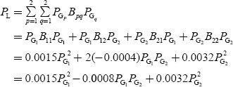
The ITL of Plant-1 is

Penalty factor of Plant-1:

The ITL of Plant-2 is
and penalty factor of plant-2 is
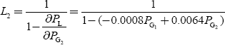
Condition for optimum operation is

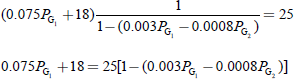
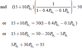
or 0.15PG1 − 0.02PG2 = 7 (3.21)
and

or 0.02PG1 − 0.24PG2 = −9 (3.22)
Solving Equations (3.21) and (3.22),
Equation (3.21) × 0.24 ⇒ 0.036PG1 − 0.0048PG2 = 1.68
Equation (3.22) × 0.02 ⇒ 0.0004PG1 − 0.0048PG2 = −0.18
0.0356PG1 = 1.86
∴ PG1 = 52.247 MW
Substituting the PG1 value in Equation (3.21), we get
0.15(52.247) − 0.02PG1 = 7
∴ PG2 = 41.852 MW
Transmission loss, PL |
= |
0.0015(52.247)2 − 0.0008 (52.247)(41.852) + 0.0032(41.852)2 |
|
= |
7.95 MW |
Total load, PD |
= |
PG1 + PG2 − PL |
|
= |
52.247 + 41.852 − 7.95 = 86.149 MW |
Example 3.4: The cost curves of two plants are
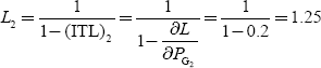
The loss coefficient for the above system is given as B11 = 0.0015/MW, B12 = B21 = –0.0004/MW, and B22 = 0.0032/MW. Determine the economical generation scheduling corresponding to λ = 25 Rs./MWh and the corresponding system load that can be met with. If the total load connected to the system is 120 MW taking 4% change in the value of λ, what should be the value of λ in the next iteration?
Solution:
Given that the cost curves of two plants are
the incremental costs are
Transmission loss, ![]()
For two plants, n = 2 and we have
The ITL of Plant-1 is

The ITL of Plant-2 is
The penalty factor of Plant-1 is

and the penalty factor of Plant-2 is
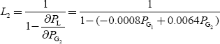
The condition for optimum operation is
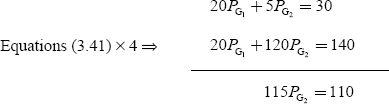
or 1.09PG1 − 0.024PG2 = 10 (3.23)
and
or 0.024PG1 − 0.292PG2 = −15 (3.24)
Solving Equations (3.23) and (3.24), we get
Equation (3.23) × 0.024 ⇒ 0.02616PG1 − 0.000576PG2 = 0.24
Equation (3.24) × 1.09 ⇒ 0.02616PG1 − 0.31828PG2 = −16.36
0.3177PG1 = 16.6
∴ PG2 = 52.25 MW
Substituting the PG1 value in Equation (3.23), we get
1.09PG1 − 0.024(52.25) = 10
∴ PG1 = 10.325 MW
Transmission loss, PL |
= |
0.0015(10.325)2 − 0.0008 (10.325)(52.25) + 0.0032(52.25)2 |
|
= |
8.465 MW |
The corresponding system load, PD |
= |
PG1 + PG2 − PL |
|
= |
10.325 + 52.25 − 8.465 = 54.11 MW |
For 4% change in value of λ, Δλ = 4% of 30 = 1.2 Rs./MWh
New load connected to system, PD = 120 MW
Change in load, ΔPD = 120 – 54.11 = 65.89 MW
Here, change in load, ΔPD > 0; hence, to get an optimum dispatch decrement λ by Δλ,
New value of λ = λ′ = λ – Δλ = 30 – 1.2 = 28.8 Rs./MWh.
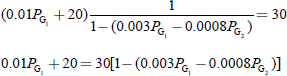
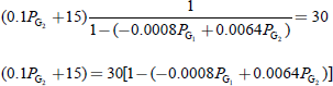
Example 3.5: A system consists of two power plants connected by a transmission line. The total load located at Plant-2 is as shown in Fig. 3.4. Data of evaluating loss coefficients consist of information that a power transfer of 100 MW from Station-1 to Station-2 results in a total loss of 8 MW. Find the required generation at each station and power received by the load when λ of the system in Rs. 100/MWh. The IFCs of the two plants are given by
Solution:
Total loss is

FIG. 3.4 Illustration for Example 3.5
Since n = 2, we have
Since power transfer of 100 MW from Plant-1 to Plant-2 (i.e., PG1 = 100 MW), PG2, P21, B22 = 0
∴ PL = B11P2G1
Given: PL = 8 MW
∴ 8 = B11 (100)2
⇒ B11 = 8 × 10⁻⁴ MW−1
∴ PL = 8 × 10⁻⁴ P2G1
and the penalty factor of Plant-1 is
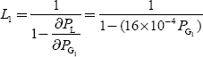
And the penalty factor of Plant-2 is
Now, the condition for optimality is
For λ = 100 Rs./MWh
or 0.12PG1 + 65 = 100(1 − 16 × 10−4 PG1)
or 0.12PG1 + 0.16PG1 = 100 − 65
0.25PG1 = 35
amd 0.25PG2 + 75 = 100
Power received by the load |
= |
(PG1 + PG2) − losses |
|
= |
125 + 100 − {8 × 10⁻⁴ × P2G1} |
|
= |
125 + 100 − {8 × 10−4 × 1252} |
|
= |
225 − 12.5 |
|
= |
212.5 MW |
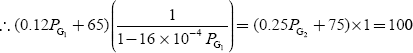
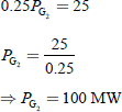
Example 3.6: For Example.3.5, with 212.5 MW received by the load, find the savings in Rs./hr obtained by co-ordinating the transmission losses rather than neglecting in determining the load division between the plants.
Solution:
By co-ordinating the losses to supply a load of 212.5 MW, the real-power generations at Plants 1 and 2 should be 125 and 100 MW, respectively.
When losses are neglected, total load = 212.5 MW is to be distributed between the two plants most economically. Condition for optimality,

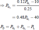
Since the losses are not co-ordinated but neglected, we have
By solving, we get
PG1 |
= |
1,659.8 MW and 190.15 MW |
PG1 |
= |
1,659.8 MW ⇒ is not to be required to overcome that power demand PD |
∴ PG1 |
= |
190.15 is to be required |
and PG2 |
= |
0.48 × 190.15 − 40 |
|
= |
51.27 MW |
∴Power generation: with losses are being co-ordinated, PG1 = 125 MW, PG2 = 100 MW with losses are not being co-ordinated, PG1 = 190.15 MW, PG2 = 51.27 MW.
Increase in cost of Plant-1 when losses are co-ordinated:

Increase in cost of Plant-2, because increase in generation:
Savings in Rs./hr by co-ordinating the losses = 5,466.67 – 4,576.17 = 890.50 Rs./hr.
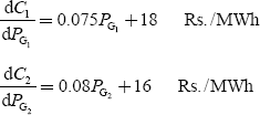
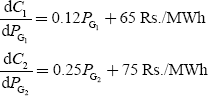
Example 3.7: On a system consisting of two generating plants, the incremental costs in Rs./MWh with PG1 and PG2 in MW are
The system is operating on economic dispatch with PG1 = PG2 = 500 MW amd ![]() Find the penalty factor of Plant-1.
Find the penalty factor of Plant-1.
Solution:
Given that the system operates on economic dispatch with pG1 = pG2 = 500 MW, the condition for this optimal operation when considering the transmission loss is
and also given that ITL of Plant-2,
The penalty factor of Plant-2,

∴ For optimal condition,
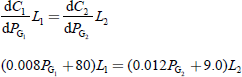
or |
[(0.008 × 500) + 80] L1 = (0.012 × 500 + 9.0)1.25 |
or |
12 L1 = 18.75 |
or |
L1 = 1.5625 |
∴ Penalty factor of Plant-1 = 1.5625.
Example 3.8: Determine the incremental cost of received power and the penalty factor of the plant shown in Fig. 3.5 if the incremental cost of production is
Solution:
The penalty factor
∴ Cost of received power

FIG. 3.5 Illustration for Example 3.8
Example 3.9: A 2-bus system consists of two power plants connected by a transmission line as shown in Fig. 3.6.
The cost-curve characteristics of the two plants are:
C1 = 0.015P2G1 + 18PG1 + 20 Rs./hr
C1 = 0.03P2G2 + 33PG2 + 40 Rs./hr
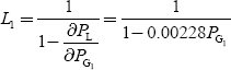
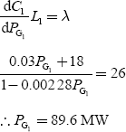
When a power of 120 MW is transmitted from Plant-1 to the load, a loss of 16.425 MW is incurred. Determine the optimal scheduling of plants and the load demand if the cost of received power is Rs. 26/MWh. Solve the problem using co-ordination equations and the penalty factor method approach.
Solution:
For two units, PL = pG1B11pG1 + 2pG1B12pG2 + pG2B21pG1
.Since the load is located at Bus-2 alone, the losses in the transmission line will not be affected by the generator of Plant-2.
i.e., B12 = B21 = 0 and B22 = 0
∴ PL = B11P2G1 (3.25)
16.425 = B11 × 1202
B11 = 0.00114 MW−1
Using the co-ordination equation method:
The co-ordination equation for Plant-1 is

FIG. 3.6 Illustration for Example 3.9
Substitute Equations (3.27) and (3.28) in Equation (3.26); then the equation for Plant-1 becomes
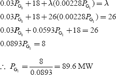
The co-ordination equation for Plant-2 is

∴ Equation (3.29) becomes

∴ The transmission loss, PL |
= |
B11P2G1 |
|
= |
0.00114 × (89.6)2 |
|
= |
9.15 MW |
∴ The load, PD |
= |
PG1 + PG2 − PL |
|
= |
89.6 + 66.67 − 9.15 = 147.12 MW |
Penalty factor method:
The penalty factor of Plant-1 is
Now the condition for optimality is
The penalty factor of Plant-2,

The transmission loss, PL |
= |
B11P2G1 |
|
= |
0.00114 × (89.6)2 |
|
= |
9.15 MW |
∴ The load, PD |
= |
PG1 + PG2 − PL |
|
= |
89.6 + 66.67−9.15 = 147.12 MW. |
Example 3.10: Assume that the fuel input in British thermal unit (Btu) per hour for Units 1 and 2 are given by
C1 = (8PG1 + 0.024P2G1 + 80)106
C2 = (6PG1 + 0.024P2G2 + 120)106
The maximum and minimum loads on the units are 100 and 10 MW, respectively. Determine the minimum cost of generation when the following load is supplied as shown in Fig. 3.7. The cost of fuel is Rs. 2 per million Btu.

FIG. 3.7 Illustration for Example 3.10
Solution:
- When the load is 50 MW:
Condition for the economic scheduling is

0.048PG1 + 8 = 0.08PG2 + 6
0.048PG1 − 0.08PG2 = −2 (3.30)
and PG1 + PG2 = 50 (3.31)
By solving Equations (3.30) and (3.31), we get
pG1 = 15 625 MW
pG2 = 34 375 MW
∴ C1 = 210.868 million Btu/h
C2 = 373.5 million Btu/h
- When the load is 150 MW,
From Equation (3.30), 0.048PG1 − 0.08PG2 = −2 (3.32)
PG1 + PG2 150 (3.33)
By solving Equations (3.32) and (3.33), we get
pG1 = 78 126 MW
pG2 = 71 874 MW
and C1 = 851.496 million Btu/hr
C2 = 757.87 million Btu/hr
∴ Total cost = Rs. (210.868 + 373.5 + 851.496 + 757.87) × 2
= Rs. 52,649.61/hr.
Example 3.11: Two power plants are connected together by a transmission line and load at Plant-2 as shown in Fig. 3.8. When 100 MW is transmitted from Plant-1, the transmission loss is 10 MW. The cost characteristics of two plants are
Find the optimum generation for λ = 22, λ = 25, and λ = 30.
Solution:
C1 = 0.05P2G1 + 13PG1
C2 = 0.06P2G2 + 12PG2
The IFC characteristics are

The transmission power loss, ![]()
Here n = 2,
PL = B11P2G1 + B22P2G2 + 2B12PG1PG2
Since the load is connected at Bus-2 and the power transfer is from Plant-1 only, B22 = 0 and B12 = 0.
∴ PL = B11P2G1
10 = B11(100)2
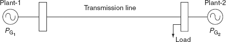
FIG. 3.8 Single line diagram representing two power plants connected by a transmission line
The ITL of Plant-1 is
The penalty factor of Plant-1 is
![]() (∵ the transmission power loss is not the function of PG2)
(∵ the transmission power loss is not the function of PG2)
The penalty factor of Plant-2 is
For optimality, when transmission losses are considered, the condition is
or 0.0144PG1 = 9
∴ PG1 = 62.5 MW,
and (0.12PG2 + 12)1 = 22
∴ PG2 = 83.33 MW
Similarly, we have
For λ = 25,
pG1 = 80 MW, pG2 = 108.33 MW
For λ = 30,
pG1 = 106.25 MW, pG2 = 150 MW
Example 3.12: For Example 3.11, the data for the loss equations consist of the information that 200 MW transmitted from Plant-1 to the load results in a transmission loss of 20 MW. Find the optimum generation schedule considering transmission losses to supply a load of 204.41 MW. Also evaluate the amount of financial loss that may be incurred if at the time of scheduling transmission losses are not co-ordinated. Assume that the IFC characteristics of plants are given by
Solution:
PL = B11P2G1 + 2B12PG1PG2 + B22P2G2
∴ The load is at Plant-2, hence B2 = B22 = 0
∴ PL = B11P2G1
And given that PG1 = 200 MW, PL = 20 M

The penalty factor of Plant-1 is
The penalty factor of Plant-2 is
For optimality,

⇒ 0.025PG1 = (1 − 0.001PG1)(0.05PG2 + 16)
⇒ 0.025PG1 = (0.05PG2 − 0.00005PG1PG2 + 16 − 0.016PG1)
0.041PG1 − 0.05PG2 + 0.00005P2G1PG2 = 16 (3.34)
and PG1 + PG2 = PD + PL
PG1 + PG2 = 204.41 + 0.0005P2G1
⇒ PG1 + PG2 − 0.0005P2G1 = 204.41 (3.35)
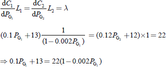
By solving Equations (3.34) and (3.35), we get
If the transmission losses are not co-ordinated, we have

While in the system, a power balance equation always holds good.
PG1 + PG2 − PD − PL = 0
PG1 + PG2 − 204.41 − 0.0005P2G1 (3.37)
By solving Equations (3.36) and (3.37), we get
pG1 = 172.91 MW
and pG2 = 46.45 MW and PL = 0 0005p2G1 = 14 95 MW
From the results, it is clear that if the transmission losses are co-ordinated, the load on Plant-1 is increased from 133.3 to 172.91 MW.
Increase in fuel cost of Plant-1 is
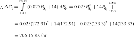
The load on Plant-2 is decreased from 80 to 46.45 MW. The decrease in the fuel cost of Plant-2 is

The net fi nancial loss |
= |
∆C1 − ∆C2 = 706.15 − 642.70 |
|
= |
63.45 Rs./hr |
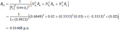
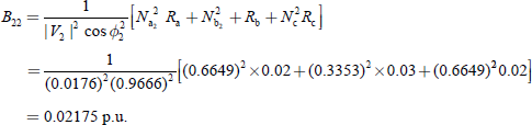
Example 3.13: For the system shown in Fig. 3.9, with Bus-1 as the reference bus with a voltage of 1.0 ∟0° p.u., find the loss formula (Bpq) coefficients if the branch currents and impedances are:
Ia = (1.00 – j0.15) p.u.; Za = 0.02 + j0.15 p.u.
Ib = (0.50 – j0.05) p.u.; Zb = 0.03 + j0.15 p.u.
Ic = (0.20 – j0.05) p.u.; Zc = 0.02 + j0.25 p.u.
If the base is 100 MVA, what will be the magnitudes of Bpq coefficients in reciprocal MW?
Solution:
The assumption in developing the expression for transmission loss is that all load currents maintain a constant ratio to the total current:
i.e.,
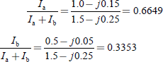
∴ The current distribution factors:
where Ia1 is the current in branch ‘a’ when Plant-1 is in operation; and Ia2 the current when Plant-2 is in operation.
Na1 = 0.6649; Na2 = 0.6649
Nb1 = 0.3353; Nb2 = 0.3359
Nc1 = –0.3353; Nc2 = 0.6649
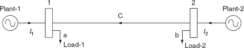
FIG. 3.9 Illustration for Example 3.13
Voltage at Bus-1 = V1 = 1.0 ∠0° p.u. = (1.0 + j 0.0) p.u.
The bus voltage at Bus-2 is
V2 = V1 + Ic Zc
= (1.00 + j 0.0) + (0.20 – j 0.05) (0.02 + j 0.25)
= 1.0165 + j 0.049 = 1.0176 ∠2.76
The plant current are
IG1 |
= |
Ia − Ic = (1.00 − j 0.15) − (0.20 − j 0.05) = 0.80 − j0.10 = 0.8062 ∠ − 7.11° |
IG2 |
= |
Ib + Ic = (0.50 − j 0.10) + (0.20 − j 0.05) |
|
= |
(0.70 − j 15) = 0.7519 ∠ − 12.09° |
The plant currents are in the form of
I1 = I1 ∠σ1
I2 = I2 ∠σ2
∴ σ1 = −7.1° and σ2 = −12.09°
cos (σ2 − σ1) = cos 4.99° = 0.996
The plant p.f.s are
cos φ1 = cos 7.1° = 0.9923
cos φ2 = cos (angle between V2 and IG2)
= cos (2.76° + 12.09°) = 0.9666
or
or
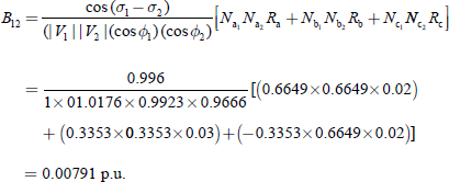
or
Example 3.14: For Example 3.13, find the ITL at the operating conditions considered.
Solution:
Transmission power loss, PL = B11P2G1 + B22P2G2 + 2B12PG1PG2


The ITL of Plant-1 is


FIG. 3.10 Illustration for Example 3.15
Example 3.15: For the system shown in Fig. 3.10, with Bus-3 as the reference bus with a voltage of 1.2 ∠0o p.u., find the loss formula (Bpq) coefficients of the system in p.u. and in actual units, if the branch currents and impedances are
Ia = 2.5 – j1.0 p.u.; Za = 0.02 + j 0.08 p.u.
Ib = 1.8 – j 0.6 p.u.; Zb = 0.03 + j 0.09 p.u.
Ic = 1.5 – j 0.5 p.u.; Zc = 0.013 + j 0.05 p.u.
Id = 3.0 – j 1.0 p.u.; Zd = 0.015 + j 0.06 p.u.
Consider that the base has 100 MVA.
Solution:
The assumption in developing the expression for transmission loss is that all load currents maintain a constant ratio to the total current.

∴ Current distribution factors are
Na1 = 1; |
Na2 = 0 |
Nb1 = 0.575; |
Nb2 = 0.425 |
Nc1 = −0.425; |
Nc2 = 0.575 |
Nd1 = 0.425; |
Nd2 = 0.575 |
The bus voltage at reference Bus ‘3’ = 1.2 + j 0.0 p.u.
The bus voltage at Plant-1, |
V1 |
= |
Vref + Ia Za |
|
|
= |
1.2 + j 0.0 + (2.2 − j 1) (0.02 + j 0.08) |
|
|
= |
1.342 ∠ 7.7° p.u. |
The bus voltage at Plant-2, |
V2 |
= |
Vref + Ic Zc |
|
|
= |
1.2 + (1.5 + j 0.5) (0.013 − j 0.05) |
|
|
= |
1.246 ∠ 3.15° p.u. |
The current phase angles at the plants = (I1 = Ia, I2 = Id + Ic)
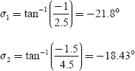
The plant power factors are
cos φ1 = cos (7.7o + 21.8o) = 0.87
cos φ2 = cos (3.5o + 18.43o) = 0.928
The loss coefficients are


For obtaining the loss coefficient values in reciprocal megawatts, the loss coefficients in p.u. must be divided by the base value (i.e.,100 MVA):

Example 3.16: A system consists of two generating plants with fuel costs of
|
C1 |
= |
0.05P2G1 + 20PG1 + 1.5 |
and |
C2 |
= |
0.075P2G2 + 22.5PG2 + 1.6 |
The system operates on economical dispatch with 100 MW of power generation by each plant. The ITL of Plant-2 is 0.2. Find the penalty factor of Plant-1.
Solution:
Given |
C1 |
= |
0.05P2G1 + 20PG1 + 1.5 |
|
C2 |
= |
0.075P2G2 + 22.5PG2 + 1.6 |
|
PG1 |
= |
PG2 = 100 MW |
and
The penalty factor of Plant-2,
Incremental fuel cost of Plant-1 ![]()
Incremental fuel cost of Plant-2 ![]()
For optimality, the condition is

⇒ (0.1PG1 + 20)L1 |
= |
(0.15PG2 + 22.5)1.25 |
(0.1×100 + 20) L1 |
= |
(0.15 × 100 + 22.5) 1.25 |
|
= |
(37.5) (1.25) |
∴ 30 L1 |
= |
46.875 |
or L1 |
= |
1.5625 |
i.e., the penalty factor of Plant-1 = L1 = 1.5625.
Example 3.17: Two thermal plants are interconnected and supply power to a load as shown in Fig. 3.11.
The following are the incremental production costs of the plants:

where pG1 and pG2 are expressed in p.u. in 100-MVA base. The transmission loss is given by
PL = 0.1P2G1 + 0.2P2G2 + 0.1PG1PG2 p.u.
If the incremental cost of received power is 50 Rs./MWh, find the optimal generation.
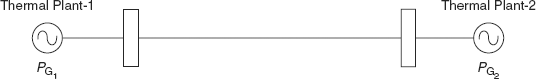
FIG. 3.11 Illustration or Example 3.17
Solution:
Given:
and |
PL |
= |
0.1P2G1 + 0.2P2G2 + 0.1PG1PG2 p.u. |
(3.38) |
Generally, |
PL |
= |
B11P2G1 + B22P2G2 + 2B12PG1PG2 |
(3.39) |
Comparing the coefficients of Equations (3.38) and (3.39), we get
Incremental cost of received power, λ = 50 Rs./MWh
The condition for optimum allocation of total load when transmission losses are considered is
The ITL of Plant-1 is
The ITL of Plant-2 is

The penalty factor of Plant-1,

The penalty factor of Plant-2,
∴ For optimum operation:
or |
20 + 10PG1 = 50 − 10PG1 − 5PG2 |
|
or |
10PG1 + 10PG2 + 5PG2 = 30 |
|
|
20PG1 + 5PG2 = 30 |
(3.40) |
Solving Equations (3.40) and (3.41), we have
∴ PG1 = 0.95652 p.u.
Substituting the pG2 value in Equation (3.40), we get
20pG1 + 5(0.95652) = 30
or 20pG1 + 4.7826 = 30
∴ pG1 = 1.26087 p.u.
Substituting the pG1 and pG2 values in Equation (3.38), we have
PL |
= |
0.1 (1.26087)2 + 0.2 (0.95652)2 + 0.1 (1.26087) (0.95652) |
|
= |
0.158979 + 0.182986 + 0.12060 |
|
= |
0.46256 p.u. |
|
= |
0.46256 × 100 = 46.256 MW |
PG1 in MW = p.u. valur × base MVA
|
PG1 |
= |
1.2608×100 |
|
|
= |
126.08 MW |
and |
PG2 |
= |
95.652 MW |
Example 3.18: A power system operates an economic load dispatch with a system λ of 60 Rs./MWh. If raising the output of Plant-2 by 100 kW (while the other output is kept constant) results in increased power losses of 12 kW for the system, what is the approximate additional cost per hour if the output of this plant is increased by 1 MW?
Solution:
For economic operation:
If the Plant-2 output is increased by 1 MW, i.e., ∂PG2 = 1 MW, the additional cost, ∂C2 = ?
Given:
λ = 60 Rs./MWh, ∂PG2 = 100 kW, and ∂PL = 12 kW:
The penalty factor of Plant-2,

The fuel cost when the output is increased by 1 MW is
∂C2 = 52.817 × dPG2 = 52.817 × 1 = 52.817 Rs./hr
Example 3.19: A power system is supplied by only two plants, both of which operate on economical dispatch. At the bus of Plant-1, the incremental cost is 55 Rs./MWh and at Plant-2 is 50 Rs./MWh. Which plant has the higher penalty factor? What is the penalty factor of Plant-1 if the cost per hour of increasing the load on system by 1 MW is 75 Rs./hr?
Solution:
Given
The cost in Rs./hr to increase the total system load by 1 MW is called system λ:
λ = 25 Rs./MWh
or
∂PG1 = 1 MW and Rs./hr = 75 (given)
For economical operation, both plants operating at common λ, i.e., λ = 75 Rs./MWh
and

Therefore, L2 is greater than L1.
KEY NOTES
- When the energy is transported over relatively larger distances with low load density, the transmission losses in some cases may amount to about 20–30% of the total load. Hence, it becomes very essential to take these losses into account when formulating an economic dispatch problem.
- Consider the objective function:
Minimize the above function subject to the equality and inequality constraints.
Equality constraints
The real-power balance equation, i.e., total real-power generations minus the total losses should be equal to real-power demand:
Inequality constraints
The inequality constraints are represented as:
- In terms of real-power generation as
PGi (min) ≤ PGi ≤ PGi(max)
- In terms of reactive-power generation as
QGi (min) ≤ QGi ≤ QGi(max)
- In addition, the voltage at each of the stations should be maintained within certain limits.
i.e., Vi(min) ≤ Vi ≤ Vi(max)
- Current distribution factor of a transmission line w.r.t a power source is the ratio of the current it would carry to the current that the source would carry when all other sources are rendered inactive i.e., the sources that do not supply any current.
- If the system has ‘n’ number of stations, supplying the total load through transmission lines, the transmission line loss is given by

- The coefficients B11, B12 and B22 are called loss coefficients or B-coefficients and are expressed in (MW)−1.
- The transmission loss is expressed as a function of real-power generations.
- The incremental transmission loss is expressed as
 .
. - The penalty factor of any unit is defined as the ratio of a small change in power at that unit to the small change in received power when only that unit supplies this small change in received power and is expressed as

- The condition for optimality when transmission losses are considered is
SHORT QUESTIONS AND ANSWERS
- State in words the condition for minimum fuel cost in a power system when losses are considered.
The minimum fuel cost is obtained when the incremental fuel cost of each station multiplied by its penalty factor is the same for all the stations in the power system.
- Define the current distribution factor.
The current distribution factor of a transmission line with respect to a power source is the ratio of the current it would carry to the current that the source would carry when all other sources are rendered inactive, i.e., the sources that are not supplying any current.
- Write the expression for the total transmission loss in terms of real-power generations when n = 2.
For n = 2,
- In the study of an optimum allocation problem, what are the considerations that you will notice regarding equality and inequality constraints in the case of transmission loss consideration and why are reactive-power constraints taken?
Equality constraints,

Inequality constraints,
PGi (min) ≤ PGi ≤ PGi (max) and
QGi (min) ≤ QGi ≤ QGi (max)
Vi (min) ≤ Vi ≤ Vi (max)
Reactive-power constraints are to be taken since the transmission losses are functions of real and reactive-power generations and also the voltage at each bus.
- What are the assumptions considered in deriving the transmission loss expression?
The following assumptions are to be considered for deriving the transmission loss expression:
- All lines in the system have the same
 ratio.
 - All the load currents have the same phase angle.
- All the load currents maintain a constant ratio to the total current.
- The magnitude and phase angle of bus voltages at each station remain constant.
- All lines in the system have the same
- Write the transmission loss expression for the kth line, if there are two generating stations in terms of station voltages, real-power generations, and their power factors.
- A simple two-plant system has the IC’s that are
dC1/dpG1 = 0.01pG1 + 2.0
dC2/dpG2 = 0.01pG2 + 1.5 and the total load on the system is distributed optimally between two stations as pG1 = 60 MV and pG2 = 110MW, corresponding to λ = 2.6 and the loss coefficients of the system are given as
p
q
Bpq
1
1
0.0015
1
2
–0.0015
2
2
0.0025
Determine the transmission loss.
Transmission loss
=
B11 P2G1 + 2B12 PG1 PG2 + B22 P2G2
=
(0.0015) (60)2 + 2(− 0.0015)
× (60 × 110) + (0.0025)
× (110)2 = 25.75 MW
- What is your analysis by considering the optimization problem with and without transmission loss consideration?
To get the solution to optimization problem, i.e., to allocate the total load among various units:
When transmission losses are neglected, the condition is

i.e., the IC of all the units must be the same.
When transmission losses are considered, the condition is

i.e., the product of IC of any unit and its penalty factor gives the optimum solution.
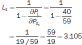
- Find the penalty factor of the plant shown in Fig. 3.12.
Here,
pG1
=
59 MW
PD
=
19 MW

FIG. 3.12 Illustration for Question number 9
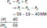
Penalty factor,
- Write the expression for transmission loss in terms of Bmin coefficients when there are three generating stations.
- Write the condition for optimality when losses are taken into consideration.

i.e.,

- Find the penalty factors of both the plants shown in Fig. 3.13.
Given: pG1 = 125 MW
pG2 = 75 MW, B11 = 0.0015
Since the load is at Station-2, the transfer of power to the load is from only Station-1 and hence B12 = B22 = B21 = 0
PL = B11P2G1 + 2B22PG1PG2 + B22P2G2
∴ PL = B11P2G1

FIG. 3.13 Illustration for Question number 12
= (0.0015) (125)2
= 0.0015 × P2G1
Penalty factor of Station-1,
Penalty factor of Station-2,
- Define the optimization problem when transmission losses are considered.
- What do you mean by ITL and penalty factor of the system? Write expressions for them.
ITL = Incremental transmission loss =

It is defined as the ratio of the change in real-power loss to the change in real-power generation.
- Why are the reactive-power constraints to be considered as inequality constraints in solving an optimization problem when transmission losses are considered?
The transmission loss is a function of real and reactive-power generations since reactive power is proportional to the square of the voltage.
- If the fuel cost in Rs./hr of a power station is related to the power generated in MW by C1 = 0.0002P3G + 0.06P2G + 300, what is the incremental fuel cost at PG = 200 MW?
- What are the points that should be kept in mind for the solution of economic load dispatch problems when transmission losses are included and co-ordinated?
The following points should be kept in mind:
- Although the incremental production cost of a plant is always positive, ITL can be either positive or negative.
- The individual units will operate at different incremental production costs.
- The generation with highest positive ITL will operate at the lowest incremental production cost.
MULTIPLE-CHOICE QUESTIONS
- In the economic operation of a power system, the effect of increased penalty factor between a generating plant and system load center is to:
- Decrease the load on the generating plant.
- Increase the load on the plant.
- Hold the plant load constant.
- Decrease the load first and then increase.
- In a power system in which generating plants are remote from the load center, minimum fuel costs occur when:
- Equal incremental costs are maintained at the generating station buses.
- Equal incremental costs are referred to system load center.
- Equal units are operated at the same load.
- All the above.
- Unit of penalty factor is:
- Rs.
- MW–1.
- Rs./MWh.
- No units.
- Unit commitment of more number of generating units is done using:
- Gradient method.
- Non-linear programming method.
- Dynamic programming.
- All the above.
- Economic dispatch is done first by ___________ and then by___________.
- Unit commitment and then load scheduling.
- Load scheduling and then unit commitment.
- Either (a) or (b).
- Unit commitment and load frequency control.
- Transmissiion losses are about:
- 50% of the total generation.
- 100% of the total generation.
- 5–15% of the total generation.
- None of these.
- In optimal scheduling of hydro-thermal units, the objective is:
- In optimal generation scheduling, the co-ordination equation for all ‘i’ values is:
- ICi = λi.
- ICi = λi Li.
- ICi = λi / Li.
- ICi = λi + Li.
- Transmission loss by B-coefficients is PL = __________
- PTBP.
- PTB.
- BP.
- All.
- The condition for optimality with consideration of transmission loss is:
- The incremental fuel costs in Rs./hr of all the units must be the same.
- The incremental fuel costs in Rs./hr of all the units must be the same.
- The incremental transmission losses in Rs./MWh of all the units must be the same.
- The incremental fuel cost of each multiplied by its penalty factor must be the same for all plants.
- Expression for transmission loss is derived using ______________ method.
- Kron’s.
- Penalty function.
- Kirchmayer’s.
- Kuhn-Tucker.

- The equality constraint, when the transmission line losses are considered, is:
- Transmission loss is:
- A function of real-power generation.
- Independent of real-power generation.
- A function of reactive-power generation.
- A function of bus voltage magnitude and its angle.
- In Kron’s method,
- Reduce the system to an equivalent system with a single hypothetical load.
- Reduce the system to an equivalent system without any load.
- Reduce the system to an equivalent system with a large number of loads.
- Enhance the system to an equivalent system with no power loss.
- The derivation of transmission line loss is not based on which assumption?
- All the load currents maintain a constant ratio.
- All the lines in the system have different
 ratios.
 - All the load currents have same phase angle.
- The power factor at each station remains constant.
- The loss coefficient B12 is given by:
- Which of the following is correct?
- The penalty factor of the ith station is:
 approximate penalty factor ith plant is expressed as:
- The incremental transmission loss is:
 is called the co-ordination equation because:
- It co-ordinates ITL with IC.
- It co-ordinates ITL with penalty factor.
- It co-ordinates real-power generation with reactive-power generation.
- It co-ordinates bus voltage magnitude with IC.
- The incremental cost of received power in Rs./MWh of the ith plant is:
- In solving optimization problem with transmission loss consideration, the condition for optimality is obtained as:
- The IC of all the plants must be the same.
- The IC of each plant multiplied with its penalty factor must be the same for all the plants.
- The IC of each plant divided by its penalty factor must be the same for all the plants.
- The IC of each plant subtracted from its penalty factor must be the same for all the plants.
- The matrix form of transmission loss expression is:
- The exact co-ordination equation of the ith plant is:
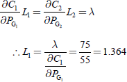
- The optimization problem is solved by the computational method with the expression for pGi which is given as:
- The penalty factor of the plant shown in Fig. 3.14 is:
- 5.
- 5.25.
- 1.25
- 12.5

FIG. 3.14 Illustration for Question number 28
- The incremental cost of received power for the above plant if
 Rs./MWh is:
- 1.25.
- 16.82.
- 16.00.
- 12.80.
- For Fig. 3.15, what is the penalty factor of the second plant if a power of 125 MW is transmitted from the first plant to load with an incurred loss of 15.625 MW?
- 24.
- 1.25.
- Zero.
- 1.
- To derive the transmission loss expression, which of the following assumptions are to be taken into consideration?
- All the lines in the system have the same R/X ratio.
- P.f. at each station remains constant.
- All the load currents maintain constant ratio to the total current.
- All the load currents have their own different phase angles.
- (i) and (ii).
- (ii) and (iii).
- All except (iv).
- All of these.

FIG. 3.15
- In deriving the expression for transmission power loss, which of the following principles are used?
- Thevinin’s theorem.
- Kron’s method.
- Max. power-transfer theorem.
- Superposition theorem.
- (i) only.
- (ii) and (iii) only.
- (ii) and (iv) only.
- All except (i).
- The transmission loss is expressed as:
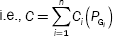
- In finding the optimal solution, the objective function is redefined as constrained objective function and is given by:


REVIEW QUESTIONS
- Derive the transmission loss formula and state the assumptions made in it.
- Obtain the condition for optimum operation of a power system with ‘n’ plants when losses are considered.
- Briefly explain about the exact co-ordination equation and derive the penalty factor.
- What are B-coefficients? Derive them.
- Explain economic dispatch of thermal plants co-ordinating the system transmission line losses. Derive relevant equations and state the significance and role of penalty factor.
- Give a step-by-step procedure for computing economic allocation of power generation in a thermal system when transmission line losses are considered.
PROBLEMS
- A system consists of two generating plants with fuel costs of:
C1
=
0.03P2G1 + 15PG1 + 1.0
and
C2
=
0.04P2G2 + 21PG2 + 1.4
The system operates on economical dispatch with 120 MW of power generation by each plant. The incremental transmission loss of Plant-2 is 0.15. Find the penalty factor of Plant-1.
- A system consists of two generating plants. The incremental costs in Rs./MWh with pG1 and pG2 in MW are:

The system operates on economic dispatch with pG1 = pG2 = 400 MW and
 . Find the penalty factor of Plant-1.
 - The cost curves of two plants are as follows:
C1 = 0.04P2G1 + 25PG2 + 120
C2 = 0.035P2G2 + 10PG1 + 160
The loss coefficient for the above system is given as B11 = 0.001/MW, B12 = B21 = – 0.0002/MW and B22 = 0.003/MW. Determine the economical generation scheduling corresponding to λ = 20 Rs./MWh and corresponding system load that can be met with. If the total load connected to the system is 110 MW taking 3.5% change in the value of λ, what should be the value of λ in the next iteration?