
11
Modeling of Prime Movers and Generators
OBJECTIVES
After reading this chapter, you should be able to:
develop the modeling of hydraulic and steam turbines
discuss reheat and non-reheat type of steam turbine configurations
develop the simplified models of a synchronous machine
discuss the application of Park’s transformation to synchronous machine modeling
study the swing equation model of a synchronous machine
11.1 INTRODUCTION
For the study of power system dynamics, the simple equivalent methods of the synchronous generators are not adequate. The accurate description of power system dynamics requires the detailed models of synchronous machines.
In this work, the above-required detailed models of synchronous machines are developed from the basic equations. The time-invariant synchronous machine equations are developed through the application of PARK’S transformation and with the use of phase variables.
The detailed synchronous machine model is derived accompanied by its representation using per unit quantities and the consideration of d-axis and q-axis equivalent circuits.
First, the most simplified model of the synchronous machine is discussed and later the detailed model is developed.
The effect of saliency is discussed. The steady-state model and dynamic model representations of a synchronous machine are discussed. Finally, the mechanical behavior of a synchronous machine is studied in the form of derivation of swing equation.
The speed control of a prime mover is essential for the frequency regulation of a power system network. This is achieved by providing a speed-governor mechanism. The parallel operation for generators requires droop characteristics incorporated in the speed governing system to secure stability and economic division of load. Hence, to maintain constant frequency, it is necessary for the prime mover control to adjust the power generation according to economic dispatch of load among various units.
The prime mover controls are classified into three different categories as:
- Primary control (speed-governor control).
- Secondary control (load frequency control (LFC)).
- Tertiary control involving economic dispatch.
In this unit, models of a hydraulic turbine with a penstock system and a steam turbine are developed. In modeling the steam turbine, six common system configurations in the form of non-reheat type and reheat type are considered.
11.2 HYDRAULIC TURBINE SYSTEM
The representation of a hydro-turbine is highly dependent on the type of prime mover because each type has different speed control mechanisms.
According to the type of head conditions, there are three types of hydro-turbines.
- Low head: Up to 100" height, specific speed (90−180 rpm), speed (100−400 rpm).
These are propeller type of reaction turbines.
- Medium head: 50"−1,000" height, specific speed (90−200 rpm), speed (100−400 rpm).
These are Francis type of reaction turbines.
- High speed: From 800" and above height, specific speed (3−7 rpm), speed (120−720 rpm). These are of impulse type of turbines (Pelton wheel).
11.2.1 Modeling of hydraulic turbine
The transient characteristics of hydro-turbines are obtained by the dynamics of water flow in the penstock. A hydraulic turbine with a penstock system is as shown in Fig. 11.1.
Let l be the length of the penstock in m, Q the discharge of water to the turbine in m3/s, ν the velocity of water discharge in m/s, and H the operating head in m.
For a particular change in load, let ΔH be the p.u. change in head, ΔN the p.u. change in speed, Δ X the p.u. change in turbine gate opening, ΔQ the p.u. change in water discharge, and ΔT the p.u. change in turbine torque.
It has been proved that
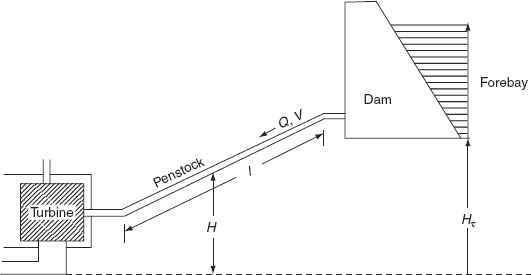
FIG. 11.1 Hydraulic turbine with penstock system
where Z is the normalized penstock impedance, τe the elastic limit of penstock, and s the complex frequency = σ + jω.
According to first-order PADE’s approximation, we have

where the time constant tw is called the water starting time or water time constant.
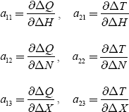
The changes in flow and torque of the turbine about a steady-state condition can be represented by the following linearized equations:
where a11, a12, a13, a21, a22, and a23 are constants and are expressed as
The change in turbine torque due to the speed changes can be neglected in comparison to other changes since the change in speed is relatively small.
∴ ΔQ = a11ΔH + a13ΔX
ΔQ = a21ΔH + a23ΔX
∴ By using Equations (11.2) and Equations (11.3), we have

For an ideal turbine with valve opening X0,
|
a11 |
= |
0.5X0 |
|
a12 |
= |
0 |
|
a13 |
= |
1.0 |
|
a21 |
= |
1.5X0 |
|
a22 |
= |
− 1.0 |
|
a23 |
= |
1.0 |
At full-load, X0 = 1.0 p.u.
Equations (11.5) is the transfer function of classical hydraulic turbine of penstock model.
The approximate linear models for hydro-turbines are as shown in Fig. 11.2.

FIG. 11.2 (a) Linearized model of hydraulic turbine; (b) linearized model of an
ideal hydraulic turbine
The input PGV for the hydraulic turbine is given from the speed governor. It is the gate opening expressed in p.u.
The value of τω lies in the range of 0.5 s − 5.0 s. the typical value of τω is around 1.0 s.
11.2.1.1 Calculation of water time constant (τω)
Water time constant is associated with the acceleration time for water in the penstock between the turbine inlet and the forebay or between the turbine inlet and the surge tank if it exists.
The water time constant τω is given by
![]()
where l is the length of penstock in m, ν the velocity of water flow in m/s, HT the total head in m, and g the acceleration due to gravity in m/s2.
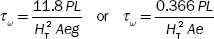
In terms of power generated by the plant ‘P’, the water time constant τw is expressed as
![]()
or
![]()
where P is the generated electrical power in kW and is given as
![]()
where A is the average penstock area in m2 and e is the product of efficiencies of turbine and generator:
i.e., e = ηturbine × ηgenerator
11.3 STEAM TURBINE MODELING
The two common steam turbine system configurations are:
- Non-reheat type.
- Reheat type.
11.3.1 Non-reheat type
A simple non-reheat type turbine is modeled by a single time constant.
The functional block diagram representation of a non-reheat type of steam turbine is as shown in Fig. 11.3.
The approximate linear model of the non-reheat steam turbine is shown in Fig. 11.4.
Here, PGV represents the power at the gate of the valve outlet, τCH the steam-chest time constant, and Pm the mechanical power at the turbine shaft.

FIG. 11.3 Block diagram representation of a non-reheat type of steam turbine
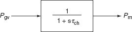
FIG. 11.4 Approximate linear model of a non-reheat steam turbine
11.3.2 Reheat type
There are mainly two configurations and they are:
- Tandem compound system configuration.
- Cross-compound system configuration.
These two configurations are further classified into the following types:
- Tandem compound, single reheat type.
- Tandem compound, double reheat type.
- Cross-compound, single reheat type with two low-pressure (LP) turbines.
- Cross-compound, single reheat type with single LP turbine.
- Cross-compound, double reheat type.
A tandem compound system has only one shaft on which all the turbines are mounted. The turbines are of high pressure (HP), low pressure LP, and intermediate pressure (IP) turbines. Sometimes, there may be also a very high pressure (VHP) turbine mounted on the shaft.
The functional block diagram representations of tandem compound reheat system configurations and their linear model representations are shown in Fig. 11.5−Fig. 11.8.
11.3.2.1 Tandem compound single reheat system
The tandem compound single reheat system is shown in Fig. 11.5 and Fig. 11.6.
All compound steam turbines use governor-controlled valves, at the inlet to the HP turbine, to control the steam flow. The steam chest, reheater, and cross-over piping introduce delays. These time delays are represented by:
τCH = Steam-chest time constant (from 0.1 to 0.4 s)
τRH = Reheat time constant (from 4 to 11 s)
τCO = Cross-over time constant (from 0.3 to 0.5 s)
The fractions of total turbine power are represented by:
FHP = Fraction of HP turbine power (typical value is 0.3)
FIP = Fraction IP turbine power (typical value is 0.3)
FLP = Fraction of LP turbine power (typical value is 0.4)
11.3.2.2 Tandem compound double reheat system
The tandem compound double reheat system is shown in Figs. 11.7 and Figs. 11.8.
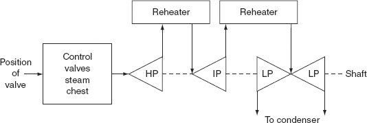
FIG. 11.5 Functional block diagram representation—tandem compound single reheat system

FIG. 11.6 Approximate linear model—tandem compound single reheat system

FIG. 11.7 Functional block diagram representation—tandem compound double reheat system
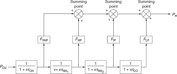
FIG. 11.8 Approximate linear model—tandem compound double reheat system
The time delays are represented by:
τRH1 = first reheat time constant
τRH2 = second reheat time constant
11.3.2.3 Cross-compound single reheat system (with two LP turbines)
The cross-compound single reheat system with two LP turbines is shown in Figs. 11.9 and 11.10.
11.3.2.4 Cross-compound single reheat system (with single LP turbine)
The cross-compound single reheat system with a single LP turbine is shown in Figs. 11.11 and 11.12.
11.3.2.5 Cross-compound double reheat type
The cross-compound double reheat-type system is shown in Figs. 11.13 and 11.14.
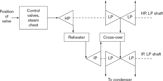
FIG. 11.9 Functional block diagram representation

FIG. 11.10 Approximate linear model

FIG. 11.11 Functional block diagram representation

FIG. 11.12 Approximate linear model
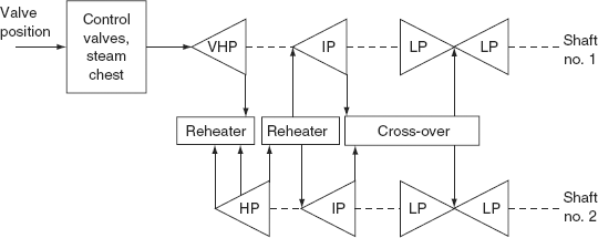
FIG. 11.13 Functional block diagram representation
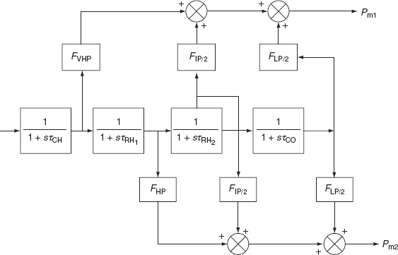
FIG. 11.14 Approximate linear model
11.4 SYNCHRONOUS MACHINES
The synchronous machine is the main or basic component of the electrical power system. It may operate either as a generator or as a motor. In power system operation, the synchronous machine is often required to supply power at power factors other than unity, which necessitates the supply or absorption of reactive power.
A synchronous machine consists of two basic parts: the stator and the rotor. The two basic rotor designs are salient pole type and non-salient-pole type.
11.4.1 Salient-pole-type rotor
In this type of rotor, the poles project from the rotor and exhibit a narrow air gap under the pole structure and a wider air gap between the poles. This type of rotor structure is shown in Fig. 11.15.
11.4.2 Non-salient-pole-type rotor
It consists of a cylindrical rotor as shown in Fig. 11.16, often made from a single steel forging, in which the field winding is embedded in longitudinal slots machined in its structure.
The mathematical modeling of a synchronous machine is complicated because of its multitude of windings, all characterized by time-varying self-inductances and mutual inductances.
11.5 SIMPLIFIED MODEL OF SYNCHRONOUS MACHINE (NEGLECTING SALIENCY AND CHANGES IN FLUX LINKAGES)
The most simplified model of a synchronous generator for the purpose of transient stability studies is a constant voltage source behind proper reactance. The voltage source may be sub-transient, transient, or steady state and the reactance may be the corresponding reactances.

FIG. 11.15 Salient-pole-type rotor structure

FIG. 11.16 Non-salient-pole-type rotor structure
In this model, saliency and changes in the flux linkages are neglected. However to understand this model, let us consider a synchronous generator operating at no-load before a 3-ϕ short circuit is applied at its terminals. The current flowing in the synchronous generator just after the 3-ϕ short circuit occurs at its terminals is similar to the current flows in an R–L circuit when an ac voltage is suddenly applied. Hence, the current will have both the AC (i.e., steady state) component as well as the dc (i.e., transient) component, which decays exponentially with the time constant L/R. If the dc component is neglected, the oscillograph of the AC component of the current that flows in the synchronous generator just after the fault occurs will have the shape as shown in Fig. 11.17.
Just after the fault, the current is maximum as the air gap flux, which generates voltage, is maximum at the instant the fault occurs than a few cycles later as the armature reaction flux produced due to a very large lagging current in the armature provides nearly a demagnetizing effect.
From Fig. 11.17, let OA be the peak value of symmetrical AC current (neglecting DC component), also known as peak value of the sub-transient current:
∴ RMS value of sub-transient current ![]() (11.6)
(11.6)
Now, if the first few cycles, where the current decrement is very fast, are neglected and the current envelope is extended up to zero time, the intercept OB is obtained:
OB = Peak value of the transient current
∴ RMS value of transient current ![]() (11.7)
(11.7)
However, the steady-state value of the short-circuit current (i.e., sustained value of short-circuit current) ![]() (11.8)
(11.8)
Since the excitation is a constant from no-load to the instant when the 3-ϕ short circuit occurs, the excitation voltage ‘Eg’ in the synchronous generator will remain constant and is known as an ‘open-circuit voltage or the no-load induced emf’, and is represented as shown in Fig. 11.18.

FIG. 11.17 Oscillograph of the current in the synchronous generator
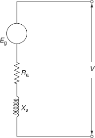
FIG. 11.18 Equivalent circuit of the synchronous generator
The phasor diagram of a non-salient-pole synchronous generator for steady-state analysis is as shown in Fig. 11.19.
Now, the machine equation becomes
where Eg is the excitation voltage (or) open-circuit voltage,
V is the full-load terminal voltage,
Ia is the armature current,
Ra is the armature resistance/phase,
Xs is the synchronous reactance/phase,
ϕ is the phase angle between V and Ia,
δ is the torque angle or power angle, and
θ the impedance angle ![]()
It is seen that the current in the synchronous generator changing from sub-transient state (I ″) to transient state (I ′) and to steady state (I) and hence the synchronous reactance of the generator must change, as Eg is constant, from sub-transient reactance (X ″) to transient reactance (X ′) to steady-state reactance (X).
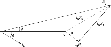
FIG. 11.19 Phasor diagram of a non-salient-pole synchronous generator for steady-state analysis
i.e.,

The armature reaction flux is produced by a large lagging current as this current is limited only by armature impedance, where winding resistance is negligible compared to synchronous reactance, Xs.
This armature reaction flux at this instant is nearly demagnetizing in nature because it acts along the direct axis of the machine; the above reactances are referred to as direct axis reactances, i.e.,
![]() direct axis sub-transient reactance
direct axis sub-transient reactance
![]() direct axis transient reactance
direct axis transient reactance
![]() direct axis component of steady state or synchronous reactance (11.11)
direct axis component of steady state or synchronous reactance (11.11)
Here I ″, I ′, and I are the sub-transient, transient, and steady-state value of short-circuit currents, respectively, and Eg is excitation (or) open-circuit voltage (or no-load induced emf) in the armature. Hence, the simplest model of the synchronous generator is a constant voltage ‘Eg’ in series with the proper impedance (or) reactance, i.e., X ″d or X ′d or Xd as shown in Fig. 11.20.

FIG. 11.20 Simplified model of synchronous generator by
neglecting the saliency and flux linkage changes
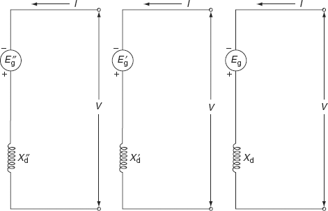
FIG. 11.21 Representation of synchronous generator
When the synchronous machine connected to the power system is operating at load before the fault occurs, the synchronous generator is represented by an appropriate voltage source behind the respective reactances as shown in Fig. 11.21.
This modeling (or) representation can easily be obtained for any fault in the power system with the help of Thevenin’s equivalent circuit, from which it is clear that the flux linkages and hence the internal voltage of the machine remain constant, but only its phase angle changes.
Now, the machine equations of the model of Fig. 11.21 will be expressed as
E″g = V + jIX″d
E′g = V + jIX′d
Eg = V + jIXd (11.12)
where Eg", Eg′ and Eg are sub-transient, transient or steady-state excitation voltages of the synchronous generator, respectively. V is the terminal voltage of the synchronous generator, and I is the current in the synchronous generator.
For the synchronous motor, Equations (11.12) may obtain the following formation.
E″g = V + jIX″d
E′g = V + jIX′d
Eg = V + jIXd (11.13)
11.6 EFFECT OF SALIENCY
The salient-pole rotor is shown in Fig. 11.15. It has a direct axis of rotor-field winding, i.e., d-axis and quadrature axis, i.e., the q-axis of the rotor-field winding. The d-axis and the q-axis revolve with the rotor, while the magnetic axes of the three stator phases remain fixed.
At the instant of time, θ is the angle from the axis of Phase-a to the d-axis. The corresponding angle from the Phase-b axis to the d-axis is θ + 240° or θ − 120°. The angle from the Phase-c axis is θ + 120°. As the rotor turns, θ varies with time, with a constant rotor angular velocity, ω, i.e., θ = ωt.
In order to include the effect of saliency, the simplest model of synchronous machine can be represented by a fictitious voltage ‘Eq’ located at the q-axis. The d-axis is taken along the main pole axis while the q-axis lags the d-axis by 90°. Then the voltage Eq is expressed in terms of full-load terminal voltage V and full-load armature current Ia as
where Xq is the quadrature axis synchronous reactance.
The equivalent circuit and phasor diagram for the case of effect of saliency are given in Figs. 11.22(a) and (b).
The excitation voltage (or) open-circuit voltage will be calculated as
Eg = V + Ia Ra + j Iad Xd + j Iaq Xq (11.15)
where Xd = Xl+Xad and Xq = Xl+Xaq. Xd is the direct axis armature synchronous reactance,
Xq the quadrature axis armature synchronous reactance,
Xad the d-axis component of armature magnetizing reactance, and
Xaq the q-axis component of the armature magnetizing reactance.

FIG. 11.22 Effect of saliency; (a) equivalent circuit; (b) phasor diagram
Xad corresponds to the d-axis component of the armature reaction flux, ϕad, and Xaq corresponds to the q-axis component of the armature reaction flux ϕaq.
Now, the phasor diagram including the effect of saliency is drawn as shown in Fig. 11.23.
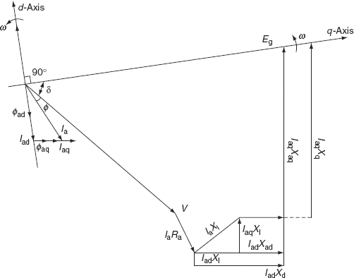
FIG. 11.23 Phasor diagram of synchronous machine including the effect of saliency
11.7 GENERAL EQUATION OF SYNCHRONOUS MACHINE
The synchronous machine has at least four windings, three on stator carrying AC and one on rotor with DC excitation.
When a coil has an instantaneous voltage V applied across its terminals and a current ‘i’ that flows from a positive terminal into the coil, the governing equation becomes
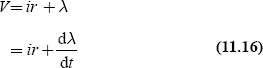
Hence, the instantaneous terminal voltage V of any winding will be in the form,
V = ± Σ ir ± Σ λ⋅
where λ is the flux linkage (it may be represented by the symbol Ψ), r the resistance of the winding, and i the current with positive direction of stator current flowing out of the generator terminal.
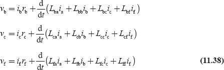
For the three stator windings a, b, and c, the voltage equations are

and for rotor-field winding,
![]()
In practice, ra = rb = rc = r
∴ λ = Li,
Equation (11.16) can be written as
11.8 DETERMINATION OF SYNCHRONOUS MACHINE INDUCTANCES
The 3-ϕ synchronous machine without damper windings may be considered as a set of coupled circuits formed by the 3-ϕ windings and rotor-field windings as shown in Fig.11.24.
In the above circuit, there are self-inductances and mutual inductances, which vary periodically with the angular rotation of a rotor.
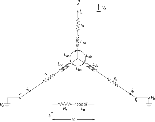
FIG. 11.24 Circuit diagram of 3-ϕ, synchronous machine
11.8.1 Assumptions
The following assumptions are usually made to determine the nature of the machine inductances to develop the detailed model of the synchronous machines:
- The self-inductance and mutual inductance of the machine are independent of the magnitude of winding currents because the magnetic saturation is neglected. Thus, the machine is assumed to be magnetically linear.
- The shape of the air gap and the distribution of windings are such that all the above inductances may be represented as constants plus sinusoidal functions of electrical rotor positions.
- Slotting effects are ignored. Distributed windings comprise finely spread conductors of negligible diameter.
- Magnetic materials are free from hysterisis and eddy current losses.
- The machine may be considered without damper windings. If the damper winding is present, then its influence may be neglected.
- Higher order time and space harmonics are neglected.
11.9 ROTOR INDUCTANCES
In this section, we shall discuss rotor self-inductance and stator to rotor mutual inductances in detail.
11.9.1 Rotor self-inductance
The stator, i.e., armature has a cylindrical structure. Hence, the self-inductance of the rotor field winding ‘f ’ will not depend upon the position of the rotor and will be a constant one.
i.e., Lff = self-inductance of rotor-field winding = constant
11.9.2 Stator to rotor mutual inductances
The stator to rotor mutual inductances will vary periodically with β. The mutual inductance between the field winding and any armature phase is the greatest when the d-axis coincides with the axis of that phase. Figure 11.25 shows the effect of field winding on mutual inductances.
Consider the example, the mutual inductance between the field winding and Phase-a (Mf) will be maximum at β = 0 and at β = 90° and negative maximum (− Mf) at β = 180° and zero again at β = 270°.
Accordingly, with space m.m.f. and flux distribution assumed to be sinusoidal, the mutual inductance between the field winding and Phase-a (Laf) can be expressed as
Laf = Lfa = Mf cos β
Based on the above, the similar expressions for Phases-b and c can be obtained directly by replacing β with (β − 120°) and (β+120°), respectively,
i.e., Laf = Lfa = Mf cos β
Lbf = Lfb = Mf cos(β − 120°)
Lcf = Lfc = Mf cos(β + 120°) (11.19)

FIG. 11.25 Effect of field winding on mutual inductances
11.10 STATOR SELF-INDUCTANCES
The self-inductance of any stator phase is always positive but varies with the position of the rotor. It is the greatest when the d-axis of the field coincides with the axis of the armature phase and being least when the q-axis coincides with it. There will be a second-harmonics variation because of different air-gap geometry along the d and q-axes. For example, the self-inductance of Phase-a (Laa) will be a maximum for β = 0 and a minimum for β = 90° and maximum again for β = 180° and so on.
When Phase ‘a’ is excited, with space harmonics ignored, the m.m.f. wave of phase ‘a’ will be a cosine wave (space distribution) centered on the Phase-a-axis as shown in Fig. 11.26.
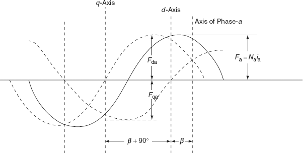
FIG. 11.26 The m.m.f. wave of Phase-a with its d-axis and q-axis components
The peak amplitude of this m.m.f. wave of Phase ‘a’ is
where Na is the effective turns/phase and ia the instantaneous current in Phase ‘a’.
Let us resolve this m.m.f. wave into two-component sinusoidal space distributions, one centered on the d-axis (Fda) and the other on the q-axis (Fqa).
The peak amplitudes of these two resolved components are
The advantage of resolving m.m.f. is that two components m.m.f. waves act on specific air-gap geometry in their respective axes.
The fundamental air-gap fluxes per pole along the two axes are, accordingly,
where Þd is the permeance along the d-axis and Þq the permeance along the q-axis.
These are known as machine constants and their values can be found from a flux plot for specific machine geometry.
Let ϕga be the air-gap flux linking with Phase-a and be expressed as
ϕga = ϕga cos β − ϕqa sin β (11.25)
= Fa (Þd cos2 β + Þq sin 2 β)
Since the air-gap flux linkage, λga = ϕga Na
If ϕla represents the leakage flux of Phase ‘a’, which does not cross the air gap, then the flux linkages of Phase ‘a’ due to leakage flux only are
λla = ϕla Na = FaÞlNa = Na2iaÞl
where Þl is the constant leakage permeance of armature Phase ‘a’.
Therefore, the total flux linkage of Phase a can be expressed as
λa = λga + λla
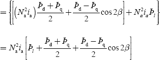
Since by definition, the inductance is the proportionality factor relating flux linkages to current, the self-inductance of Phase ‘a’ due to the air-gap flux when only Phase ‘a’ is excited, will be
where ![]() is a constant term,
is a constant term,
![]() is the amplitude of second-harmonics variation
is the amplitude of second-harmonics variation
For Phase ‘b’, the variation of self-inductance is similar, except that the maximum value occurs when the d-axis coincides with the Phase b-axis. The self-inductances of Phase ‘b’ and Phase ‘c’ can be obtained by replacing β by (β − 120°) and (β + 120°), respectively:
Lbb = Ls + Lm cos 2 (β − 120°)
= Ls + Lm cos(2β − 240°)
= Ls + Lm cos(2β + 120°) (11.30)
Lcc = Ls + Lm cos 2 (β + 120°)
= Ls + Lm cos(2β + 240°)
= Ls + Lm cos(2β − 120°) (11.31)
i.e., the stator self-inductances are obtained as
Laa = Ls + Lm cos 2β
Lbb = Ls + Lm cos(2β + 120°)
Lcc = Ls + Lm cos(2β − 120°)
11.11 STATOR MUTUAL INDUCTANCES
The mutual inductances between stator phases will also exhibit a second-harmonics variation with β because of the rotor shape. The mutual inductance between two phases can be found by evaluating the air-gap flux linking one phase when another phase is excited. For example, the mutual inductance between Phases a and b, Lab = Lba, can be obtained by evaluating ϕgba linking Phase ‘b’ when only Phase ‘a’ is excited. ϕgba can be computed from Equation (11.24) by replacing β with (β − 120°) as
ϕgba = ϕda cos (β − 120°) − ϕqa sin (β − 120°)
= Fa [Þd cos β cos(β − 120°) + Þq sin β sin(β − 120°)]
The mutual inductance between Phase-a and Phase-b due to the air-gap flux is then
where ![]()
Similarly, the mutual inductances of stator Lbc and Lca can be obtained as
i.e., the stator mutual inductances are expressed as
Lab = − Ms + Lm cos(2β − 120°)
Lbc = − Ms + Lm cos(2β)
Lca = − Ms + Lm cos(2β + 120°)
Here, Ls, Lm, and Ms are regarded as known machine constants and are determined either by tests or calculated by designed. All the inductances except Lff are functions of β and thus they are time-varying.
11.12 DEVELOPMENT OF GENERAL MACHINE EQUATIONS — MATRIX FORM
From the knowledge of the above time-varying inductances, the general machine equations are developed. If a motoring mode is considered, then for any winding, the general equation relating the applied voltage of the input current is
![]()
In terms of self-inductance and mutual inductance, the flux linkages are expressed as
λa = Laaia + Labib + Lacic + Lafif
λb = Lba ia + Lbb ib + Lbcic + Lbf if
λc = Lca ia + Lcb ib + Lccic + Lcf if
λf = Lfa ia + Lfb ib + Lfcic + Lff if (11.37)
Equations (11.17) can be modified as
Write the above equations in a compact matrix form:
where


and
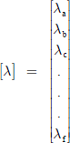
The vectors of the flux linkages are proportional to the currents with matrix of self-inductance and mutual inductance as the proportionality factor.
where

i.e.,

The inductance L is symmetric, i.e., Lab = Lba, etc.
If the expressions of inductances of Equations (11.19) – (11.36) are substituted in Equations (11.38), the solution of resulting equations can be simplified by a transformation, known as Blondel’s transformation, which is also generally called Park’s transformation.
11.13 BLONDEL’S TRANSFORMATION (OR) PARK’S TRANSFORMATION TO ‘dqo’ COMPONENTS
Equations (11.37)–(11.41) are a set of differential equations describing the behavior of machines. However, the solution of these equations is complicated since the inductances are the functions of rotor angle ‘β’, which in turn, is a function of time.
The complication in getting the solution can be avoided by transferring the physical quantities in the armature windings through a linear, time-dependent, and power-invariant transformation called Park’s transformation.
This transformation is based on the fact that the rotating field produced by 3-ϕ stator currents in the synchronous machine can be equally produced by 2-ϕ currents in a 2-ϕ winding. Let us consider the 3-windings for the three phases a, b, and c of a synchronous machine as shown in Fig. 11.27.
When all the three phases are excited, the total stator m.m.f’.s that act along the d-axis and q-axis are
Fds = Fa cos β + Fb cos(β − 120°) + Fc cos(β + 120°)
= Na [ia cos β + ib cos(β − 120°) + ic cos(β + 120°) (11.42)
and Fqs = Fa sin β − Fb sin(β − 120°) + Fc sin(β + 120°)
= Na [ia sin β − ib sin(β − 120°) − ic sin(β + 120°) (11.43)
Let us consider two fictitious windings, one placed on the d-axis and the other on the q-axis, as shown in Fig. 11.28.

FIG. 11.27 The m.m.f.’s of 3-ϕ windings and their resultant m.m.f.’s along the d-axis and the q-axis
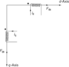
FIG. 11.28 Fictitious coils on d and q-axes
The winding on the d-axis rotates at the same speed as the rotor-field winding and remains in such a position that its axis always coincides with the direct axis of the rotor field. Hence, the instantaneous current id gives the same m.m.f. Fds on this axis as do the actual three instantaneous armature phase currents flowing in the actual armature windings. Similarly, the current iq flowing in the winding on the q-axis gives the same m.m.f. Fqs on this axis as do the actual three instantaneous armature phase currents flowing in the actual armature windings.
In order to transform quantities in the f-a-b-c axes into the f-d-q-0 axes, the constraints of the system forming the basis of the transformation may be obtained by viewing the currents, m.m.f.’s, voltages, and flux linkages in the two axes. The currents in view of Equations (11.42) and (11.43) are
if = if
id = Kd [iacos β + ib cos(β − 120°) + ic cos(β + 120°)]
iq = Kq [ia cos(β + 90°) + ib cos(β − 120° + 90°) + ic cos(β + 120° + 90°)]
= − Kq [ia sin β + ib sin(β − 120°) + ic sin(β + 120°)] (11.44)
A new current, known as zero-sequence current, which does not produce any rotating field is introduced and is expressed as
where Kd, Kq, and K0 are constants.
Now in this system, there are three original phase currents ia, ib, and ic and three field currents id, iq, and io. For the ungrounded star connection or for the balanced 3-ϕ condition, the sum of phase currents is zero and hence io must also be zero.
Equations (11.44) and (11.45) are expressed in a matrix form as

In a more compact matrix form, Equation (11.46) can be expressed as
This is known as PARK’s transformation (or Blondel’s transformation).
where

and

and is known as PARK’s transformation matrix (or Blondel’s transformation matrix).
The effect of Park’s transformation is simply to transform all stator quantities from phases a, b, and c into new variables, the frame of reference of which moves with the rotor, i.e., the Park’s transformation matrix [P]dqof transforms the field of phasors to the field of d-q-o-f components and it is a linear, time-dependent matrix.
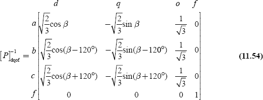
11.14 INVERSE PARK’S TRANSFORMATION
The inverse transformation, which transforms the d-q-o-f quantities into the phase quantities, is expressed as
where
11.15 POWER-INVARIANT TRANSFORMATION IN ‘F-D-Q-O’ AXES
The total instantaneous power delivered to the motor is
When f-d-q-o axes’ quantities are substituted for the phase quantities by using Equation (11.50) and by further manipulation, these results give power in terms of new quantities as
Equation (11.52) gives the true power associated with the armature of the new system. This power invariance is preserved if
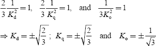
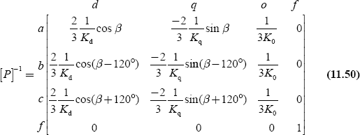
Since the angle between the d-axis and the Phase-a axis is β, and the q-axis has been chosen ahead of the d-axis, the values of Kd and Kq must be positive; hence, the selected values of the three quantities are
With these values, Park’s transformation matrix and its inverse become

Now, the transformation is called unitary transformation because the inverse of the transformation matrix is the transpose of the matrix, i.e., [P]−1 = [P*T]
i.e., Inverse of the matrix = transpose of conjugate of the matrix.
∴ The current equation of a synchronous machine equation (11.46) can be expressed as
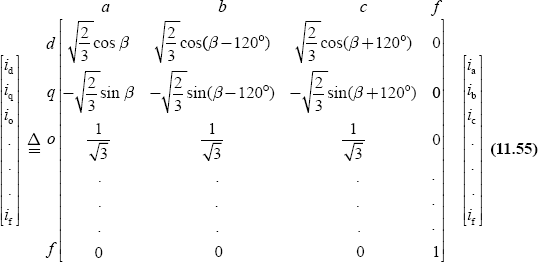
and in terms of inverse Park’s transformation, the current equations of synchronous machine can be expressed as

11.16 FLUX LINKAGE EQUATIONS
The flux linkage equations in matrix form are [λ] = [L][i]. In terms of self-inductance and mutual inductance, the flux linkages from Equation (11.37) are expressed as
λa = Laaia + Lab ib + Lacic + Laf if
λb = Lba ia + Lbb ib + Lbcic + Lbf if
λc = Lca ia + Lcb ib + Lccic + Lcf if
λf = Lfa ia + Lfb ib + Lfcic + Lff if
In matrix form, it is expressed as
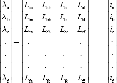
In vector form, it can be expressed as
The flux linkages of f-d-q-o coils in terms of four currents are obtained upon transforming both sides by using the transformation matrix [P] and its inverse [P]−1 as follows:
|
[λ]dqof |
= |
[P] [λ]abcf (11.58) |
|
|
= |
[P]{[L]abcf[i]abcf} |
|
|
= |
[P][L]abcf[P]−1[i]dqof (11.59) |
[∵from Equation (11.56); [i]abcf = [P]−1[i]dqof

By substituting ![]() we get
we get

where |
Ld = direct axis synchronous inductance = |
|
Lq = quadrature axis synchronous inductance = |
|
Lo = zero-sequence inductance = Ls – 2Ms |
Note: The mutual inductance Laf can also be represented by Maf or M.
From Equation (11.61), we have

From Equation (11.62), it is noticed that the inductances are not functions of rotor position β. Hence, it is a greater advantage of transforming phase quantities to a suitable set of quantities of f-d-q-o-axes.
11.17 VOLTAGE EQUATIONS
The original voltage equation of a synchronous machine is
i.e.,

For transformation, let us pre-multiply both sides of Equation (11.63) by [P],
Hence,

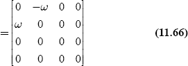
It can be shown that ![]() is a matrix with zero entries except for –ω in the first row, second column and +ω in the second row, first column,
is a matrix with zero entries except for –ω in the first row, second column and +ω in the second row, first column,
i.e.,

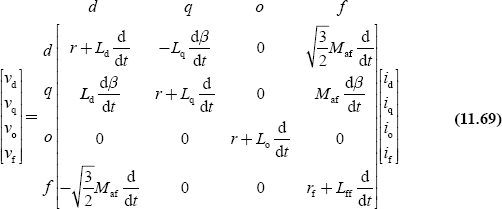
After the transformation, synchronous machine equations in matrix form become

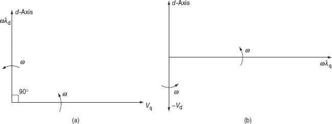
FIG. 11.29 (a) Phasor diagrams Vq versus ωλd; (b) phasor diagrams ωλq versus –Vd
∵ Ra = Rb = Rc = R
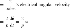
where ω = angular velocity of rotation = ![]()
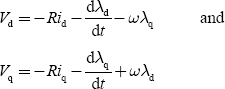
From Equation (11.67), the voltage equations obtained are

For sinusoidal steady-state conditions, the flux phasor leads the voltage phasor by 90°. This means that vq will be induced by the flux in the direct axis (ωλd); i.e., vq will be induced by (ωλd) and similarly − vd will be induced by (ωλq) as shown in Figs. 11.29(a) and (b).
11.18 PHYSICAL INTERPRETATION OF EQUATIONS (11.62) AND (11.68)
The terms ωλd and ωλq are speed voltages (flux changes in space) and the terms ![]() and
and ![]() are transformer voltages (flux changes in time). Usually, these transformer voltages are small compared with speed voltages and may be neglected. The neglected transformer voltages correspond to negligence of the harmonics and DC components in transient solution for stator voltages and currents. Negligence of harmonics and DC components in the phase current is very common in machine analysis. Neither harmonics nor DC components have a significant effect on the average torque of the machine since harmonics are usually small and DC components die away very rapidly.
are transformer voltages (flux changes in time). Usually, these transformer voltages are small compared with speed voltages and may be neglected. The neglected transformer voltages correspond to negligence of the harmonics and DC components in transient solution for stator voltages and currents. Negligence of harmonics and DC components in the phase current is very common in machine analysis. Neither harmonics nor DC components have a significant effect on the average torque of the machine since harmonics are usually small and DC components die away very rapidly.
The solutions of network equations become extremely difficult and complex when the harmonics and DC components are present in electrical quantities if the transformer voltages are included. Hence, it is preferable to approximate the associated damping torques by additional terms in the swing equation.
11.19 GENERALIZED IMPEDANCE MATRIX (VOLTAGE–CURRENT RELATIONS)
By combining Equations (11.62) and (11.68), we get
In compact form, the above matrix can be expressed as
It is observed that the impedance matrix is symmetrical in f and d-axes. It consists of two terms, one relating to transformer voltages and the second ![]() relating to speed voltages, as given below:
relating to speed voltages, as given below:

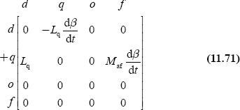
where ![]() angular speed of rotation
angular speed of rotation
11.20 TORQUE EQUATION
The speed voltages are:
- In the direct axis, λdω and
- In the quadrature axis, − λqω
Mechanical angular velocity
The total 3-ϕ power output of a synchronous machine is given by

Assume balanced but not necessarily steady-state conditions, thus v0 = 0 and i0 = 0.
From Equation (11.68),
Substituting vd and vq expressions in Equation (11.74), we get
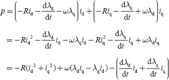
The above expression consists of three terms and they are:
- The first term represents the rate of change of stator magnetic field energy.
- The second term represents the power transferred across the air gap.
- The third term represents the stator ohmic losses.
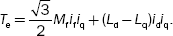
The machine torque is obtained from the second term,
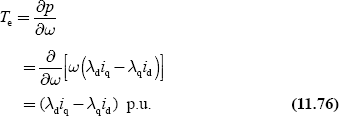
Substituting for λd and λq from Equation (11.62) in Equation (11.76), we get

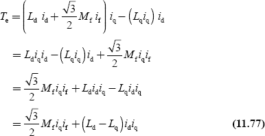
For a cylindrical rotor synchronous machine, the direct axis and quadrature axis inductances are equal, i.e., Ld = Lq:
For a salient-pole machine, there is a saliency torque:
This torque exists only because of non-uniformity in the permeance of the air gap along the d- and q-axes. This is the reluctance torque of a salient-pole machine and exists even when the field excitation is zero.
11.21 SYNCHRONOUS MACHINE—STEADY-STATE ANALYSIS
Consider a 3-ϕ synchronous machine that has three armature (stator) windings a, b, and c, one field winding ‘f ’ on the rotor with its flux in the direction of the d-axis, and one fictitious winding ‘g’ on the rotor with its flux in the quadrature axis as shown in Fig. 11.30.

FIG. 11.30 Three-phase synchronous machine with stator and rotor windings
The fictitious winding ‘g’ approximates the effect of eddy currents circulating in the iron (rotor iron in round-rotor machine and negligible in salient-pole machine) and to some extent the effect of damper windings. This fictitious winding is short circuited since it is not connected to any voltage source.
Since the electromagnetic transients in the network are much faster than the mechanical transients, the steady-state phasor solutions on the network side are performed.
11.21.1 Salient-pole synchronous machine
The phasor diagram of an overexcited salient-pole synchronous generator for lagging p.f. is shown in Fig. 11.31.

FIG. 11.31 Phasor diagram of a salient-pole synchronous generator
|
δ is the power angle or torque angle |
|
Ea the terminal voltage = va |
|
Eag the voltage due to air-gap flux |
|
Eaf the voltage due to flux produced by main rotor-field current |
|
IadXad the voltage drop across d-axis armature magnetizing reactance |
|
IaqXaq the voltage drop across q-axis armature magnetizing reactance |
|
λag the flux linkage due to net air-gap flux |
|
λagd the d-axis component of flux linkage |
|
λagq the q-axis component of flux linkage |
|
λad the flux linkage due to d-axis component of Ia |
|
λaq the flux linkage due to q-axis component of Ia |
|
xd the d-axis component of synchronous reactance = xl + xad |
|
xq the q-axis component of synchronous reactance = xl + xaq |
Figure 11.32 represents the phasors and their speeds:
|
δ is the angle between synchronously rotating reference phasor axis and q-axis |
|
ωs the synchronous speed |
|
ω the speed of rotor |

FIG. 11.32 Phasors and their speeds
From the phasor diagram shown in Fig. 11.32, we have

By applying Park’s transformation, we get
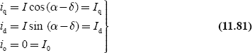
Equations (11.81) can be expressed as a phasor equation:
Iq + jId = Iej(a − δ)
= Ῑe−jδ as Ῑ I ∠ α (11.82)
For the steady-state analysis, the q-axis will be considered as the real axis and the d-axis as the imaginary axis since the voltage induced in a normal steady-state operation lies on the q-axis.
Similarly, by Park’s transformation, we get
vq = v cos(θ − δ)
vd = v sin(θ − δ)
Vo = 0
In complex notation,

To get the steady-state analysis, we make use of the following assumptions:
- Transformer voltages,
 and
and  , being small and are therefore neglected.
 - Balanced network currents and voltages are assumed.
The reasons for the above assumptions are that changes in λd and λq are very slow in time with the oscillations of angle δ and hence ![]() and
and ![]() are very small compared with ωλd and ωλq.
are very small compared with ωλd and ωλq.
Due to the above assumptions, Equations (11.62) and (11.68) can be rewritten by dropping the transformer voltage terms, zero-sequence currents, and voltages:

Substituting for λd and λq in the above equations of voltages, we get
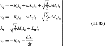
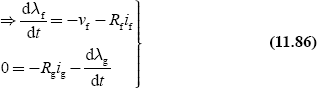
Hence, ![]()
Iq + jId = I ej(α − δ)
vq + jvd = v ej(α − δ)
11.21.2 Non-salient-pole synchronous (cylindrical rotor) machine
For this case, Xd = Xq
∴ Eaf = Ea + ia Ra + jia X1 + jia Xad
= Ea + ia Ra + jid Xd (11.87)
The equivalent circuit of a non-salient-pole synchronous machine is represented
by a source Eaf (induced emf) in series with the internal impedance Ra + jXd as shown in Fig. 11.33.
The phasor diagram is shown in Fig. 11.34. Now, the synchronous reactance is defined as Xs = Xaq + Xl, and if resistance ‘r’ is neglected, the cylindrical rotor synchronous generator is represented by the equivalent circuit as shown in Fig. 11.35.

FIG. 11.33 Equivalent circuit of non-salient-pole synchronous generator

FIG. 11.34 Phasor diagram of non-salient-pole synchronous generator
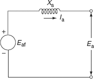
FIG. 11.35 Equivalent circuit
Now, Equation (11.87) becomes
The above relationship represents the model of the cylindrical rotor (non-salient pole) generator under steady-state conditions and of which a very useful equivalent circuit is shown in Fig. 11.35.
11.22 DYNAMIC MODEL OF SYNCHRONOUS MACHINE
In this section, we shall discuss the dynamic model of synchronous machines—salient pole synchronous generator, dynamic equations of synchronous machine, and equivalent circuit of synchronous generator—in detail.
11.22.1 Salient-pole synchronous generator—sub-transient effect
During normal steady-state conditions, there is no transformer action between stator and rotor windings of synchronous machines, as the resultant field produced by stator windings and rotor windings revolves with the same (synchronous) speed and in the same direction. However, during disturbances, the rotor speed is no longer the same as that of the revolving field produced by stator windings, which always rotates with synchronous speed. Hence, the synchronous generator becomes a transformer.
Synchronous machine dynamic equations
We have

Let Xd = ωLd = d-axis component of synchronous reactance,
Xq = ωLq = q-axis component of synchronous reactance:
and

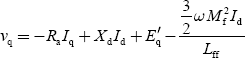
Substituting the If value in Equation (11.90), we get
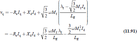
Let ![]() sub-transient voltage along the q-axis
sub-transient voltage along the q-axis
Since at this time, both windings ‘f ’ and ‘g’ are present along the d-axis then, Equation (11.91) becomes
Let ![]() transient d-axis reactance
transient d-axis reactance
Since at this time, both the d-axis component of the armature windings and the f-winding are present, Equation (11.92) becomes
Similarly, the equation of vd is given by
Substituting, ωLq = Xq, we get
We know that ![]()

Substituting Ig expression in Equation (11.94), we get
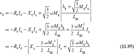
Let ![]() Transient voltage along the d-axis (since both the q-axis component and g-windings are present to give transient state) and also let
Transient voltage along the d-axis (since both the q-axis component and g-windings are present to give transient state) and also let
![]() q-axis component of transient reactance
q-axis component of transient reactance
Hence, Equation (11.95) becomes
Let ![]() direct axis open-circuit transient time constant
direct axis open-circuit transient time constant
![]() quadrature axis open-circuit transient time constant
quadrature axis open-circuit transient time constant
and also

i.e., E = Eq + jEd
Substituting Equation (11.97) in Equations (11.90) and (11.94), we get
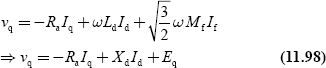
From Equations (11.93) and (11.98)
vq = − RaIq + X′dId + E′q = − RaIq + XdId + Eq
i.e., E′q = Eq + (Xd − X′d)Id (11.100)
Similarly from Equations (11.96) and (11.99), we have
vd = − RaIq + X′qIq + E′d = − RaId − XqIq + Ed
i.e., E′d = Ed − (Xq − X′q)Iq (11.101)
Figure 11.36 shows the phasor diagram of a synchronous machine under the transient state.
From the phasor diagram also we get
E′q = Eq + Id (Xd − X′d) = voltage behind the d-axis component of transient reactance
E′d = Ed − Iq (Xq − X′q) = voltage behind the q-axis component of transient reactance
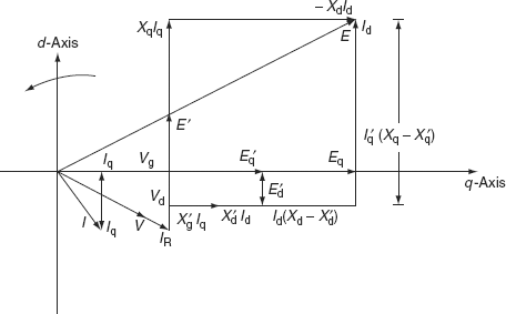
FIG. 11.36 Phasor diagram
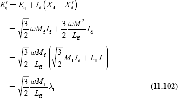
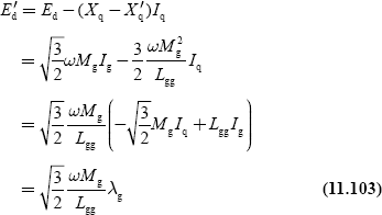
From Equations (11.102) and (11.103), we have

Therefore, from the above analysis, we get
Taking the derivative for Equation (11.105), we get


and also taking the derivative of Equation (11.106), we have

![]() q-axis component of open-circuit transient reactance time constant
q-axis component of open-circuit transient reactance time constant
i.e.,

Equations (11.93) and (11.96) can be written in the matrix form as
11.22.2 Dynamic model of synchronous machine including damper winding
The ‘f ’ and ‘g’ coils in the rotor winding produce transient effect in terms of X′d and X′q in the synchronous machine. The field coil ‘f ’ exists physically whereas the ‘g’ coil is hypothetical for representing the rotor eddy currents in the q-axis. However, it is quite difficult to calculate g-coil inductance.
The more accurate representation of synchronous machine is obtained by adding two more fictitious windings on the rotor, one along the d-axis known as ‘Kd’ winding and the other along the q-axis, known as ‘Kq’ winding. These damper windings can be approximated by two hypothetical coils, both short-circuited as there is no voltage source connected to them.
The dynamic machine equations will now be modified to include the damper windings by substituting the scalar (λf and λg) vectors:
Now in this model, the Park’s transformation will be applied with the following assumptions:
- Mutual inductances from stator coils a, b, and c (or its component ‘d’ and ‘q’ axes) to the ‘Kd’ coil is the same as ‘f ’ coil, and to the Kg coil the same as ‘g’ coil and
- Mutual inductance between ‘Kd’ coil and ‘f ’ coil (and ‘Kg’ coil and ‘g’ coil) is the same as ‘d’ component of stator coils and f-coils (or ‘q’ component of stator to ‘g’ coil).
The resultant equations after Park’s transformation are

From the above matrix representation, the modified voltage equations with the inclusion of damper windings are

The modified flux linkages with the inclusion of damper windings are obtained in the form of matrix as
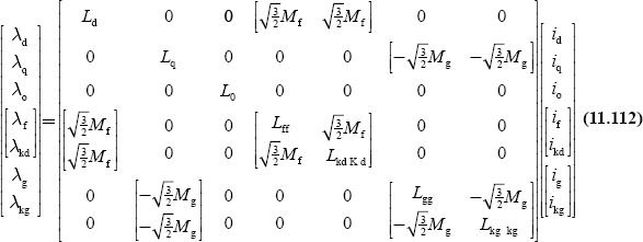
i.e., the flux linkage equations are

11.22.3 Equivalent circuit of synchronous generator—including damper winding effect
11.2.3.1 Along the d-axis
The equivalent circuit of the synchronous generator along the d-axis excluding resistances is as shown in Fig. 11.37, where Xl is the armature leakage reactance, Xad the armature magnetizing reactance, Xf the field reactance, and Xg the fictitious winding reactance.
Initially, all the reactances are in the circuit (i.e., just at the instant when the fault has occurred) and therefore, initial or sub-transient reactance, are the lowest. After some time, the g-winding (damper winding) is out of circuit as it has a very low time constant and hence we have only field winding and armature reactances in parallel. This reactance is known as transient reactance and is larger than the previous one. However, after some time, when the disturbance altogether disappears, field winding is also out of circuit and hence we have only armature reactance, (Xd = Xl + Xad) called the steady-state reactance of the circuit.

FIG. 11.37 Equivalent circuit of synchronous generator
For a more accurate representation, two more fictitious windings ‘Kd’ winding and ‘Kq’ winding are added. Hence, the equivalent circuit of the synchronous generator along the d-axis can be represented as shown in Fig. 11.38.
The parallel combination of Xad, Xf, and Xkd is known as the d-axis component of sub-transient reactance X″ad and is represented as X″ad = Xad / Xf / Xkd.
Hence, the d-axis component of the sub-transient synchronous reactance is given by
X″ d = X1 + X″ ad
This reactance is very small. After some time, as the hunting becomes less, the winding Kd is also out of circuit since it has a low time constant.
Thus, the resultant equivalent circuit becomes as shown in Fig. 11.39.
The parallel combination of reactances Xad and Xf is known as X′ad, d-axis component of transient armature reactance.
The d-axis component of transient synchronous reactance is X′d = = X1 + X′ad
Generally, X′d > X″d
Finally, when the disturbance is altogether over, there will not be hunting of the rotor and hence there will not be any transformer action between the stator and the rotor. Hence, the equivalent circuit of synchronous generator becomes as shown in Fig. 11.40.
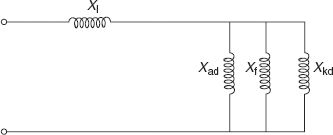
FIG. 11.38 Accurate representation of equivalent circuit of synchronous generator

FIG. 11.39 Resultant equivalent circuit of synchronous generator

FIG. 11.40 Equivalent circuit

FIG. 11.41 Equivalent circuit of synchronous generator along the q-axis
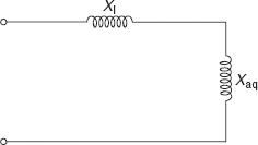
FIG. 11.42 Resultant equivalent circuit of the synchronous generator
Here, Xd = Xl + Xad and is called the direct axis component of synchronous reactance.
It is obvious that X″d < X′d < Xd.
11.2.3.2 Along the q-axis
Just after the disturbance, the equivalent circuit of the machine will become as shown in Fig. 11.41.
Here, X″q = X1 + (Xaq // Xg // Xkq)
where X″q is the q-axis component of sub-transient synchronous reactance. The value of X″q is very small.
After some time, hunting becomes less and less, both g-winding and Kq, which have a low time constant, will be out of circuit and hence the resultant equivalent circuit of the synchronous generator becomes as shown in Fig. 11.42.
Here, X′q = Xq = X1 + Xaq, where X′q is the q-axis component of transient synchronous reactance.
11.23 MODELING OF SYNCHRONOUS MACHINE—SWING EQUATION
The mechanical behavior of a synchronous machine can be established by interconnecting the electrical and mechanical sides of a synchronous machine in terms of electrical and mechanical torque. This is provided by the dynamic equation for the acceleration or deceleration of the rotor of a combined turbine and synchronous generator system, which is usually called the swing equation.
While developing a swing equation or a mechanical equation, the following basic assumptions are to be made:
- Synchronous machine rotor speed must be synchronous speed.
- The rotational power losses due to friction and windage are neglected.
- Mechanical shaft power is smooth, i.e., the shaft power is constant.
Let us consider a single rotating machine with steady-state angular speed ![]() and phase angle δ. Due to various electrical or mechanical disturbances, the machine will be subjected to differences in mechanical and electrical torque, causing it to accelerate or decelerate. Hence, during disturbance, the rotor will accelerate or decelerate with respect to the synchronously rotating air-gap m.m.f. and a relative motion begins.
and phase angle δ. Due to various electrical or mechanical disturbances, the machine will be subjected to differences in mechanical and electrical torque, causing it to accelerate or decelerate. Hence, during disturbance, the rotor will accelerate or decelerate with respect to the synchronously rotating air-gap m.m.f. and a relative motion begins.
Let θ be the angular position of the rotor at any instant ‘t’
ω the angular velocity (rad/s)
α the acceleration
δ the phase angle of a rotation machine
Tnet the net accelerating torque in a machine
Telec the electrical torque exerted on the machine by the generator
Pnet the net accelerating power
Pmech the mechanical power input
Pelec the electrical power output
J the moment of inertia for the machine
M = Jω; angular momentum of the machine in kg-m2
Jα = Tnet
Pnet = ωTnet = ω(Jα) = Mα
Consider a synchronous generator developing an electromagnetic torque Te and running at the synchronous speed ωs. If Tm is the driving mechanical torque, then under steady-state conditions, with negligible losses,
Tm = Te
A departure from the steady state due to a disturbance results in an accelerating (Tm > Te) or decelerating (Te > Tm) torque Ta on the rotor:
Ta = Tm − Te
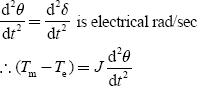
Neglecting the frictional and damping torque, from the law of rotation, we have
Now, the value of θ is continuously changing with time ‘t’. It is convenient to measure θ with respect to a reference axis, which is rotating at synchronous speed.
If δ is the angular displacement of a rotor in electrical degree from the synchronous rotating reference axis and ωs, the synchronous speed in electrical degrees, then θ can be expressed as the sum of: (i) time-varying angle ωst on the rotating axis and (ii) the torque angle δ of the rotor with respect to the rotating reference axis as shown in Fig. 11.43:

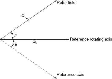
FIG. 11.43 Phasor representation of rotor-field position
and the rotor angular acceleration is obtained by differentiating the above equation again:
The torque acting on the rotor of a synchronous generator includes the mechanical input torque from the prime mover, torque due to rotational losses (i.e., friction, windage, and core loss), electrical output torque, and damping torques due to prime mover, generator, and power system.
The electrical and mechanical torques acting on the rotor are of opposite sign and are of a result of electrical input and mechanical load. By neglecting damping and rotational losses, so that accelerating torque is
Ta = Tm − Te
and multiplying with ω, we get
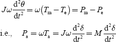
The swing equation in terms of moment of inertia or angular momentum is
∴ Swing equation is also expressed as

KEY NOTES
- The prime mover controls are classified as:
- Primary control (speed governor control).
- Secondary control (load frequency control (LFC)).
- Tertiary control involving economic dispatch.
- The transient characteristics of hydro-turbines are obtained by the dynamics of water flow in the penstock.
- The water starting time or water time constant value lies in the range of 0.5 - 5.0 s.
- Steam turbine system configurations are:
- Non-reheat type.
- Reheat type.
- Reheat type steam turbines are classified as:
- Tandem compound, single reheat type.
- Tandem compound, double reheat type.
- Cross-compound, single reheat type with two LP turbines.
- Cross-compound, single reheat type with single LP turbine.
- Cross-compound, double reheat type.
- Most simplified model of a synchronous generator for the purpose of transient stability studies is a constant voltage source behind proper reactance.
- In order to include the effect of saliency, the simplest model of a synchronous machine can be represented by a fictitious voltage ‘Eq’ located at the q-axis. The d-axis is taken along the main pole axis while the q-axis lags the d-axis by 90°.
- The stator to rotor mutual inductances will vary periodically with the angle between the q-axis and the d-axis of a synchronous machine.
- The self-inductance of any stator phase is always positive but varies with the position of the rotor. It is the greatest when the d-axis of the field coincides with the axis of the armature phase and is the least when the q-axis coincides with it.
- The effect of Park’s transformation is simply to transform all stator quantities from phases a, b, and c into new variables, the frame of reference of which moves with the rotor, i.e., Park’s transformation matrix [P]dqof transforms the field of phasors to the field of d-q-o-f components and it is a linear, time-dependent matrix.
SHORT QUESTIONS AND ANSWERS
- What is the significance of water time constant, τω?

where ΔH is the p.u. change in water head, ΔQ the p.u. change in the water discharge, τω the water time constant, τe the elastic limit of penstock, z the normalized penstock impedance, and τe known as the water time constant or water starting time.
The value of τω lies in the range of 0.5 – 5.0 s.
The typical value of τω is around 1.0 s.
- How are the transient characteristics of hydro-turbines obtained?
By the dynamics of water flow in the penstock. - The water time constant τω is associated with what time?
τω is associated with acceleration time for water in the penstock between the turbine inlet and the forebay or between the turbine inlet and the surge tank if it exists. - Write the expression for water time constant τω in terms of velocity of flow of water.

where L is the length of penstock in m, v the velocity of water flow in m/s, HT the total head in m, and g the acceleration due to gravity in m/s2.
- Write the expression for water time constant τω in terms of power generation of the plant.
where P is the power generation in

where e = ηturbine × ηgeneration
- What are the common steam turbine system configurations?
- Non-reheat system.
- reheat type.
- What are the compound system configurations of a steam turbine?
Tandem compound and cross-compound system configuration.
- What are the types of tandem compound system configuration?
Single reheat type and double reheat type.
- What are the types of cross-compound system configuration?
- Single reheat type with two LP turbines.
- Single reheat type with single LP turbines.
- Double reheat type.
- What do you mean by tandem compound reheat-type steam turbine?
Tandem compound system configuration has only one shaft on which all the turbine (are of HP, LP, and IP) types are mounted.
- What are the components that introduce the time delays and how can these delays be represented?
Steam chest, reheat, and cross-over piping are the components that introduce the time delays in the operation of steam turbines.
The time delays can be represented by:
τCH = steam-chest time constant (0.1–0.4 s).
τRH = reheat time constant (4–11 s).
τCO = cross-piping time constant (0.3–1.5 s).
- What is the most simplified model of a synchronous generator for the purpose of a transient stability study?
A constant voltage source behind a proper reactance, the voltage source may be sub-transient or steady state and the reactance may be corresponding reactance.
- Why is the reactance of the synchronous generator equivalent circuit referred to as direct axis reactance when the 3-ϕ short-circuit fault occurs?
The armature reaction flux at that instant is nearly demagnetizing in nature and because it acts along the direct axis of the machine, the equivalent circuit reactance is referred to as direct axis reactance.
- The modeling of a synchronous machine is easily obtained for any fault in a power system by which circuit?
Thevenin’s equivalent circuit.
- Write the expression for excitation voltage or open-circuit voltage of a synchronous machine for the effect of saliency.
Eq = V + Ia Ra + jIad Xd + jIaqXq.
- Write the voltage equations for the three stator windings and rotor windings in terms of flux linkages.
Va = iara + dλ a /dt.
Vb = ibrb + dλb /dt.
Vc = icrc + dλc /dt.
Vf = ifrf + dλf /dt.
- What are the assumptions usually made to determine the nature of the machine inductance to help the detailed model of synchronous machines?
- The self-inductance and mutual inductance of the machine are independent of the magnitude of winding currents because of neglecting magnetic saturation.
- The shape of the air gap and the distribution of windings are such that all the machine inductances may be represented as constant plus sinusoidal functions of electrical rotor positions.
- Slottings are ignored.
- Magnetic materials are free from hysteresis and eddy current losses.
- The machine may be considered without damper windings. If a damper winding is presented, its influence may be neglected.
- Higher time and space harmonics are neglected.
- Write the expressions for stator to rotor mutual inductances of a synchronous machine.
Laf = Lfa = Mf cos β
Lbf = Lfb = Mf cos(β − 120°)
Lcf = Lfc = Mf cos(β+120°).
- Write the expressions for stator self-inductances of a synchronous machine.
Laa = Ls+Lm cos 2β
Lbb = Ls+Lm cos(2β+120°)
Lcc = Ls+Lm cos(2β − 120°).
- Write the expressions for rotor self-inductances of a synchronous machine.
Lab = − Ms+Lm cos(2β − 120°)
Lbc = − Ms+Lm cos2β
Lca = − Ms+Lm cos(2β+120°).
- What is Park’s transformation and what is its requirement?
The behavior of a synchronous machine can be described by a set of differential equations. The solution of these differential equations is complicated since the inductances are the functions of rotor angle β, which in turn is a function of time. The complication in getting the solution can be avoided by transferring the physical quantity in the armature windings through a linear, time-dependent, and power-invariant transformer called Park’s transformation.
- In Park’s transformation, which quantities are transformed?
Quantities such as currents, m.m.f.s, voltages, and flux linkages in a b c f axes to d q o f axes are transformed.
- Express Park’s transformation matrix.

- What is the function of Park’s transformation matrix?
Park’s transformation matrix [p] transforms the field of a b c f components to the field of d q o f components.
- Park’s transformation matrix is called unitary matrix. Why?
Because the inverse of Park’s transformation matrix is the transpose of conjugate of the matrix.
[p]−1 = [p*]T
- Write the expression for the flux linkages of f d q o coils in terms of coil currents by using transformation matrix and its inverse.
[λ]dqof = [p][L]abcf [p] − 1[i]dqof.
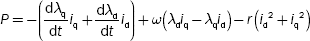
- Write the expression for 3-ϕ power output of a synchronous machine in terms of rate of flux linkages d-axis and q-axis currents.

- In the expression for 3-ϕ power output of a synchronous machine in terms of rate of flux linkages d-axis and q-axis currents, what parameters do the three terms indicate?
First term:
 represents the rate of change of stator magnetic field energies.
Second term ω(λdid − λqiq) represents the power transferred across the air gap.
Third term r(id2 + iq2) represents the stator ohmic losses.
- What is the significance of saliency torque Te = (Ld − Lq)idiq?
The saliency torque exists only because of non-uniformity in the performance of the air gap along the d-axis and the q-axis. This is the reluctance torque of a salient-pole machine and exists even when the field excitation is zero.
- What is the significance of fictitious winding ‘g’ on rotor in detailed modeling of a synchronous machine?
The fictitious winding ‘g’ on the rotor of the synchronous machine approximates the effects of eddy currents circulating in the iron currents and to some extent the effect of damper windings. This fictitious winding is short-circuited since it it not connected to any voltage source.
- What is the significance of ‘f ’ and ‘g’ coils in rotor winding in the modeling of a synchronous machine?
The ‘f ’ and ‘g’ coils in the rotor winding produce transient effect in terms of X ′d and X ′q in a synchronous machine; the field coil ‘f ’ exists physically, whereas ‘g’ coil is hypothetical for representing the rotor eddy currents in the q-axis.
- What is the significance of kd winding and kg winding in rotor winding in the modeling of a synchronous machine?
The more accurate representation of a synchronous machine is obtained by adding two more fictitious windings, f-coil and g-coil windings. One fictitious winding is known as the kd winding along the d-axis and the other along the q-axis is known as the kq axis. These two damper windings can be approximated by two hypothetical coils both short circuited as there is no voltage source connected to them.
MULTIPLE-CHOICE QUESTIONS
- The transient characteristics of hydro-turbines are obtained by:
- The dynamics of water in the reservoir.
- The dynamics of water in the penstock.
- The water head.
- None of these.
- The water time constant of hydro-turbine Tw is associated with:
- The acceleration time for water in the penstock between the turbine inlet and the forebay.
- The acceleration time for water in the penstock between the turbine inlet and the surge tank if it exists.
- Either (a) or (b).
- None of these.
- Expression for water time constant Tw in terms of power generation of the plant P is:


- Either (a) or (b).
- None of these.
- In the expression of water time constant , the term e is given as:
- e = ηturbine × ηgenerator.
- e = ηturbine /ηgenerator.
- e = ηturbine + ηgenerator.
- e = ηturbine − ηgenerator.
- The steam turbines are mainly classified into:
- HP turbines and LP turbines.
- Single and double-type turbines.
- Non-reheat and reheat-type turbines.
- None of these.
- The system where only one shaft on which all the turbines are mounted are:
- Tandem compound system.
- Cross-compound system.
- Either (a) or (b).
- Both (a) and (b).
- In the tandem compound system, the turbines mounted on a shaft are:
- Only HP type.
- IP type.
- Only LP type.
- All of these.
- In __________ type of steam turbines, the governor-controlled values are used at the inlet to control steam flow.
- Tandem compound system.
- Cross-compound system.
- Either (a) or (b).
- All compound.
- In controlling the steam flow, the time delays are introduced due to:
- Steam chest.
- Reheater.
- Cross-over piping.
- All of these.
- Match the following:
AB
(a) Steam-chest time constant (τch).
(i) 0.3–0.5 s.
(b) Reheat time constant (τRh).
(ii) 4–11 s.
(c) Cross-over time constant (τco).
(iii) 0.1–0.4 s.
(d) Water time constant (τw).
(iv) 0.5–5.0 s.
- A non-reheat type steam turbine is modeled by:
- A single time constant.
- Two time constants.
- Without time constant.
- Either (a) or (b).
- The most simplified model of a synchronous generator is:
- A constant voltage source behind proper reactance.
- A constant current source behind proper reactance.
- A variable voltage source behind reactance.
- A variable current source behind reactance.
- The armature reaction flux at the instant of fault occurs due to a very large lagging current, which is nearly ___________in nature.
- Magnetizing.
- Demagnetizing.
- Either (a) or (b).
- None of these.
- The armature reaction flux at the instant of fault occurs acts along which axis of the machine?
- Direct axis.
- Quadrature axis.
- Both (a) and (b).
- None of these.
- The most specified model representation of a synchronous generator can easily be obtained for any fault in the power system with the help of ___________ circuit.
- Norton’s equivalent.
- Thevenin’s equivalent.
- Maximum power transfer theorem equivalent.
- None of these.
- In order to include the effect of saliency, the simplest model of a synchronous machine can be represented as:
- A fictitious voltage Eq located at the q-axis.
- A fictitious voltage Ed located at the d-axis.
- A fictitious voltage Ed Eq along both the axes.
- None of these.
- The expression for Eq in terms of a full-load terminal voltage V and full-load armature current Ia is:
- Eq = V + j Ia (Ra + Xq).
- Eq = V + j Ia Ra + IaXq.
- Eq = V − Ia Ra + j IaXq.
- Eq = V + Ia Ra + jIaXq.
- For the synchronous generator, without the effect of saliency, the machine equation can be represented as:
- Eg = V + j I Xq.
- Eg = V + j I Xd.
- Eg = V − j I Xq.
- Eg = V − j I Xd.
- The expression for excitation or open-circuit voltage of the synchronous generator with the effect of saliency is:
- Eg = V + jI Xd.
- Eg = V + Ia Ra + jIa Xq.
- Eq = V + Ia Ra + jIad Xd + jIaq Xq.
- none of these.
- The synchronous machine has:
- The instantaneous terminal voltage of synchronous machine of any winding expressed in terms of flux linkages is:
- V = ir +λ.
- V = ir + jλ.
- V = ir + dλ/dt.
- none of these.
- To develop the detailed model of synchronous machine, which of the following assumptions are usually made to determine the nature of the machine inductance?
- the self-inductance and mutual inductance of machine are independent of magnitudes of winding current.
- the self-inductance and mutual inductance may be represented as constants plus sinusoidal functions of electrical rotor positions.
- slotting effects are ignored.
- magnetizing materials are free from hysteresis and eddy current losses
- (i) and (ii)
- all except (iv)
- all except (i)
- all of these
- The self-inductance of any stator phase of a synchronous machine is always ___________, but varies the position of ___________.
- positive, rotor.
- negative, rotor.
- positive, stator.
- negative, stator.
- The self-inductance of any stator phase of a synchronous machine is greater when:
- The q-axis of field coincides with the axis of armature phase.
- The d-axis of field coincides with the axis of armature phase.
- either (a) or (b).
- none of these.
- The self-inductance of any stator phase of a synchronous machine is least when:
- The q-axis of field coincides with the axis of armature phase.
- The d-axis of field coincides with the axis of armature phase.
- either (a) or (b).
- none of these.
- The expressions for self-inductances of stator phases of a synchronous machine are:
- Laa = Lm + Ls cos 2β
Lbb = Lm + Ls cos(2β + 120°)
Lcc = Lm + Ls cos(2β − 120°).
- Laa = Lm − Ls cos 2β
Lbb = Lm − Ls cos(2β + 120°)
Lcc = Lm − Ls cos(2β − 120°).
- Laa = Ls + Lm cos 2β
Lbb = Ls + Lm cos(2β + 120°)
Lcc = Ls + Lm cos(2β − 120°).
- Laa = Ls − Lm cos 2β
Lbb = Ls − Lm cos(2β + 120°)
Lcc = Ls − Lm cos(2β − 120°).
- Laa = Lm + Ls cos 2β
- The stator mutual inductances of a synchronous machine are:
- Lab = Ms + Lm cos(2β − 120°)
Lbc = Ms + Lm cos 2β
Lca = Ms + Lm cos(2β + 120°).
- Lab = Ms + Lm cos 2β
Lbc = Ms + Lm cos(2β − 120°)
Lca = Ms + Lm cos(2β + 120°).
- Lab = − Ms + Lm cos 2β
Lbc = − Ms + Lm cos(2β − 120°)
Lca = − Ms + Lm cos(2β + 120°).
- Lab = − Ms + Lm cos(2β − 120°)
Lbc = − Ms + Lm cos 2β
Lca = − Ms + Lm cos(2β + 120°).
- Lab = Ms + Lm cos(2β − 120°)
- Park’s transformation matrix is:
- linear.
- time-dependent.
- power-invariant.
- all of these.
- The fact on which Park’s transformation based is:
- the rotating field produced by 3-ϕ stator currents in the synchronous machine can be equally produced by 2-ϕ currents in 2-ϕ winding.
- the rotating field produced by 3-ϕ stator currents in the synchronous machine
can be equally produced by 1-ϕ currents
in 1-ϕ winding. - either (a) or (b).
- none of these.
- The matrix form of representation of Park’s transformation is:
- [i]dqof ≅ [P]dqof [i]abcf.
- [i]abcf ≅ [P]dqof [i]abcf.
- [i]dqof ≅ [P]abcf [i]abcf.
- [i]dqof ≅ [P]dqof [i]abcf.
- Park’s transformation matrix is:


- none of these.
- Park’s transformation matrix [p]dqof transforms:
- field of stator phasors to the field of d-q-o-f components.
- field of rotor phasors to the field of d-q-o-f components.
- field of stator phasors to the field of a-b-c-f components.
- field of rotor phasors to the field of a-b-c-f components.
- Park’s transformation matrix [p]dqof is:
- a linear matrix.
- a time-dependent matrix.
- non-linear and time-invariant matrix.
- both (a) and (b).
- Park’s transformation matrix [p]dqof is:


- none of these.
- which of the following is correct regarding to Park’s transformation?
- [P] = [P] − 1.
- [P] − 1 = [P]T.
- [P] − 1 = [P*].
- [P] − 1 = [P*]T.
- Park’s transformation matrix is called unitary transformation since:
- inverse of Park’s transformation matrix is equivalent to transpose of the matrix.
- Park’s transformation matrix is equal to transpose of the matrix.
- inverse of Park’s transformation matrix is equal to transpose of conjugate of the matrix.
- none of these.
- The flux linkages of f d q o coils are expressed in terms of Park’s transformation matrix and its inverse as:
- [λ]dqof = [P][L]abcf [P] − 1[i]dqof.
- [λ]dqof = [P][L]dqof [P] − 1[i]abcf.
- [λ]dqof = [P] − 1[L]dqof [P] [i]dqof.
- none of these.
- The expression for 3-ϕ power output of a synchronous machine is:
Which of the following is correct?
- first term represents the rate of change of stator magnetic field changes.
- second term represents the power transferred across the air gap.
- third term represents the stator ohmic losses
- all of these.
- The torque expression of a salient-pole synchronous machine is:
 .
. .
. .
. .
.
- The torque expression of a cylindrical rotor synchronous machine is:
 .
. .
.- .
 .
.
- In the dynamic model of a synchronous machine including damper windings, the more accurate representation is obtained by adding two fictitious windings on rotor, kd winding and kq winding along the d-axis and the q-axis. These damper windings are approximated as:
- two hypothetical coils both open-circuited.
- two hypothetical coils with voltage sources connected to them.
- two hypothetical coils both short-circuited as there is no voltage source connected to them.
- none of these.
REVIEW QUESTIONS
- Develop the linearized modeling of a hydraulic turbine.
- Discuss the different configurations of reheat type of steam turbines with a representation of their functional block diagrams and approximate their linear models.
- Explain the simplified model of a synchronous machine.
- Describe the effect of saliency in synchronous machine modeling.
- Derive the self-inductance and mutual inductance stator and rotor of synchronous machines.
- Explain Park’s transformation and inverse Park’s transformation.
- Develop the steady-state analysis of salient and non-salient-pole synchronous machines.
- Develop the dynamic analysis of salient and non-salient-pole synchronous machines, with and without damper windings.