
12
Modeling of Speed Governing and Excitation Systems
OBJECTIVES
After reading this chapter, you should be able to:
develop the modeling of speed-governor systems for steam and hydraulic turbines
develop the modeling of speed-governor systems with limiters
study the effect of excitation variation on synchronous machines
discuss the methods of providing excitation of synchronous machines
study the structure of a general excitation system
develop the transfer functions of various components of an excitation system
12.1 INTRODUCTION
Two important control loops are needed for the economic and reliable operation of a power system. They are:
- Load frequency control (LFC) loop (p.f. control loop) for the regulation of system frequency.
- Automatic voltage control loop (Q –V control loop) for the regulation of system voltage magnitude.
These control loops indirectly influence the real and reactive power balances in the power system network.
The LFC is achieved by the speed-governor mechanism. The basic principle of the speed-governor mechanism is that according to the load variation, the speed of the rotor shaft of the synchronous machine is varied and hence the frequency of the system is varied. This change in frequency is sensed and compared with a reference and produces a feedback signal. This feedback signal makes the variation of generated power of synchronous generator by adjusting the opening of the steam inlet valve to steam turbine or water gates in the case of a hydro-turbine. Hence, the real power balance between real power generation and real power demand is achieved. This is the basic principle of the speed-governor mechanism.
The speed governors are regarded as primary control elements in an LFC system.
With an increase in the system size due to interconnections, in normal cases, the frequency variations become very less and LFC assumes importance. However, the role of speed governors in rapid control of frequency can be underestimated.
The automatic voltage control or Q –V control is achieved by an excitation control mechanism. The main and important objective of an excitation system is to control the field current of the synchronous machine. The field current is controlled so as to regulate the generating voltage of the machine.
As the field circuit time constant is high (of the order of a few seconds), the fast control of the field current requires ‘field forcing’. Thus, the field excited should have a high ceiling voltage, which enables it to operate transiently with voltage levels that are three to four times the normal voltages. The rate of change of voltage should also be fast.
The excitation systems of synchronous machines have an extreme effect on system stability and when evaluated on the basis of an increased power carrying per increase in the system cost, they are by far the most economical source of increased stability limits.
The excitation system often contains other features such as voltage dip compensation to compensate for the voltage drop in some impedance between the generator and the rest of the network.
The functioning of LFC and automatic voltage control loops is presented in detail in Unit-VII (LFC-II).
In this unit, the modeling of speed-governing systems for steam turbines and hydro-turbines is discussed.
The effect of varying excitations on a synchronous generator, methods of providing excitation, and their block diagram representation and modeling are also discussed.
12.2 MODELING OF SPEED-GOVERNING SYSTEMS
According to the principle of control, the speed-governing systems are mainly classified into two categories, for both steam and hydraulic turbines. They are:
- Mechanical-hydraulic-controlled and
- Electro-hydraulic-controlled
In both these types, hydraulic servomotors are used for positioning the valve or gate, controlling the steam or the water flow.
12.3 FOR STEAM TURBINES
In this section, we shall discuss mechanical-hydraulic-controlled speed-governing system, electro-hydraulic-controlled speed-governing systems, and general model for speed-governing systems for steam turbines in detail.
12.3.1 Mechanical-hydraulic-controlled speed-governing systems
For a steam turbine, the mechanical-hydraulic-controlled speed-governing system consists of a speed governor, a speed relay, hydraulic servomotor, and governor-controlled valves.
The functional block diagram of a mechanical-hydraulic-controlled speed-governing system is shown in Fig. 12.1.
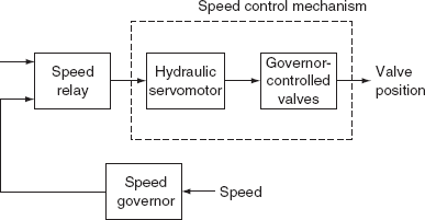
FIG. 12.1 Functional block diagram

FIG. 12.2 Approximate non-linear model representation with limits
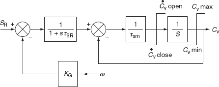
FIG. 12.3 Simplified diagram of Fig. 12.2
The approximate non-linear mathematical model can be represented by the block diagram shown in Figs. 12. 2 and 12.3.
KG is the gain of speed governor, which is the reciprocal of regulation or droop. It represents a position of an assumed linear instantaneous indication of speed produced by the speed governor.
Governor speed-changer position provides the speed regulation (SR) signal and it is determined by a system of automatic generation control.
The signal SR represents a composite load and speed reference. It is assumed to be constant over the interval of a stability study.
τSR is the time constant of speed relay. The speed relay is represented as an integrator and is provided as direct feedback.
The non-linear property of the valve is compensated by means of providing a non-linear CAM in between the speed relay, and the hydraulic servomotor.
The servomotor controls the valve's movement and is represented as an integrator with time constant τSM and is provided as direct feedback. Rate limiting of the servomotor may occur for large, rapid-speed deviations, and rate limits that are shown at the input to the integrator. The position limits that are indicated correspond to wide-open valves or the setting of a load limiter.
Generally, the non-linearities present in a speed control mechanism are neglected in the study of power system operation and controlling except for rate limits and the limits on valve position.
The typical parameters for a mechanical-hydraulic system are:
KG = 20.0
τSR = 0.1 s = speed relay time constant
τSM = 0.2–0.3 s = valve positioning servomotor time constant

12.3.2 Electro-hydraulic-controlled speed-governing systems
In this type of speed-governing systems, the mechanical components in the lower power portions are replaced by the static electronic circuits and thus provides more flexibility.
The functional block diagram representation of an electro-hydraulic speed-governing system is shown in Fig. 12.4.
The linearity of the system can be improved compared to mechanical-hydraulic-controlled system by means of providing feedback loops of steam flow and the servomotor.
The approximate mathematical model for a general EHC system is shown in Fig. 12. 5.
The typical parameters for this block diagram are:
KG = 20.0
KP = 3.0 with steam flow feedback
= 1.0 without steam flow feedback
τSM = 0.1 s
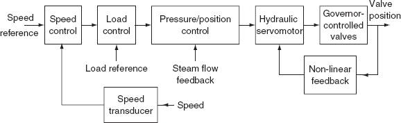
FIG. 12.4 Functional block diagram
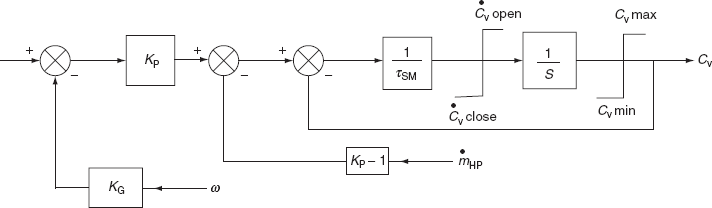
FIG. 12.5 Block diagram for approximate mathematical model

FIG. 12.6 General model of a speed-governing system for steam turbines
12.3.3 General model for speed-governing systems
A simplified, general model of speed-governing systems for steam turbines is shown in Fig. 12.6.
By the proper parameter selection, this general model represents either a mechanical-hydraulic system or an electro-hydraulic system.
This model shows the load reference as an initial power P0. This initial value is combined with the increments due to speed deviation to obtain total power PGV, subject to the time lag τ3 introduced by the servomotor mechanism.
The typical values of time constants are:
For a mechanical-hydraulic system:
τ1 = 0.2 – 0.3 s
τ2 = 0
τ3 = 0.1 s
For an electro-hydraulic system:
τ1 = τ2
τ3 = 0.025 – 0.15 s
Note that when τ1 = τ2, the value of τ1 or τ2 has no effect, as there is pole-zero cancellation.
The rate limits are nominally 0.1 p.u. per second. The nominal value of k = 100/(% steady-state SR).
12.4 FOR HYDRO-TURBINES
In this section, mechanical-hydraulic-controlled speed-governing systems, general model for a hydraulic turbine speed-governing system, and EHC-controlled speed-governing systems are discussed in detail.
12.4.1 Mechanical-hydraulic-controlled speed-governing systems
It consists of a speed governor, a unit of pilot valve and servomotor, a unit of distributor valve, and gate servomotor and governor-controlled gates.
The functional block diagram of a mechanical-hydraulic-controlled speed-governing system is shown in Fig. 12.7.
The speed-governing requirements for hydro-turbines are strongly influenced by the effects of water inertia.

FIG. 12.7 Functional block diagram representation of mechanical-hydraulic-controlled speed-governing system
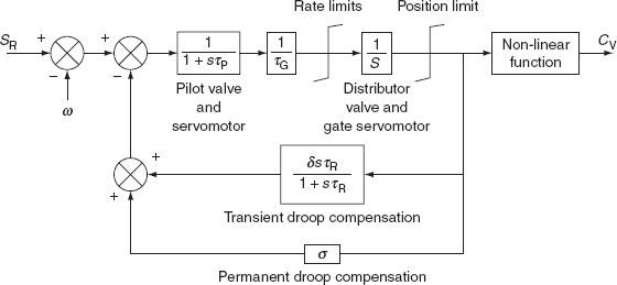
FIG. 12.8 Block diagram for approximate non-linear model
To achieve the stable performance of a speed-governing system, the dashpot feedback is required.
An approximate non-linear model for the above system is shown in Fig. 12.8.
The gate servomotor may be rate-limited for large rapid-speed excursions. However, transient droop feedback reduces the likelihood rate-limiting in stability analysis. Position limits exist corresponding to the extremes of gate opening.
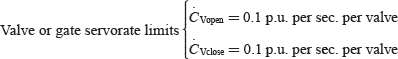
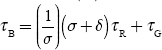
The typical parameters of a speed-governing system for hydro-turbines and their values and their ranges are given in Table 12.1, where τR is the time constant of dashpot, τG the gate time constant of gate servomotor, τP the time constant of pilot valve, δ the transient speed droop coefficient, and σ the permanent speed droop coefficient.
Typically, τR and δ are computed as
τR = 5τw
TABLE 12.1 Typical parameters of a speed-governing system for hydro-turbines
| Parameters | Typical value | Range |
|---|---|---|
τR |
5.00 |
2.5–25.0 |
τG |
0.20 |
0.2–0.40 |
τP |
0.04 |
0.03–0.05 |
δ |
0.30 |
0.2–1.00 |
σ |
0.05 |
0.03–0.06 |
and ![]()
where τw is the water starting time and H the turbine-generator inertia constant.
12.4.1.1 General Model for Hydraulic Turbine Speed-Governing System
The general model for a hydraulic turbine speed-governing system is shown in Fig. 12.9.
Let ![]()
Then τ1 and τ3 of Fig. 12.9 can be expressed approximately as
![]()
Also from Fig. 12.9, ![]() τ2 = 0
τ2 = 0
P0 is the initial power (load reference determined from automatic generation control).
PGV is the output of the governor and is expressed as power reference in p.u. It is also to be noted that K is the reciprocal of σ (steady-state SR in p.u.).
12.4.2 Electric-hydraulic-controlled speed-governing system
The low-power functions associated with speed sensing and droop compensation in a modern speed-governing system for hydro-turbines can be performed by an electronic apparatus, which results in the better performance and greater flexibility in both dead band and dead time. For interconnected system operation, however, the dynamic performance of the electric governor is necessarily adjusted to be essentially the same as that for the mechanical governor, so that a separate model is not needed.
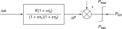
FIG. 12.9 General model for a speed-governing system for hydro-turbines
12.5 MODELING WITH LIMITS
There are two types of limiters that are different in terms of behavior:
- Wind-up limiter.
- Non-wind-up limiter.
12.5.1 Wind-up limiter
The block diagram representation of a wind-up limiter is shown in Fig. 12.10.
In this case of limiter, the output variable (y) of the transfer function G(s) is not limited and is free to vary. Hence, the limiter can be treated as a separate block whose input is ‘y’ and the output is ‘z’.
If ![]() the equations with the wind-up limiter are:
the equations with the wind-up limiter are:
![]()
If L ≤ y ≤ H, then z = y
y > H, then z = H
y < L, then z = L
where L is the lower limit of output z and H the upper limit of output z.
12.5.2 Non-wind-up limiter
In this case, the output of the transfer function G(s) is limited and there is no separate block for the limiter.
The equations are:
f = (u – y) τ
If y = H and f > 0,
y = L and F < 0
then ![]()
Otherwise, ![]()
and L ≤ y ≤ H

FIG. 12.10 Block diagram representation of a wind-up limiter
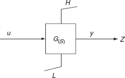
FIG. 12.11 Block diagram representation of a non-wind-up limiter
The block diagram representation of a non-wind-up limiter is shown in Fig. 12.11.
Note:
- As the output z of the limiter does not change until y comes within the limits, the wind-up limiter can change in terms of slow response.
- Generally, all integrator blocks have non-wind-up limits.
12.6 MODELING OF A STEAM-GOVERNOR TURBINE SYSTEM
While modeling the steam generators, at every instant the boiler controls and on-line frequency control equipment are to be ignored due to their slower operations.
A boiler contains a certain amount of heat stored in its hot metal and this is usually sufficient to guarantee that the demands for extra steam during system disturbances can be met.
During long-term operations, we must consider the rate of deterioration of steam conditions as a boiler having sufficient capacity of producing indefinitely only a given amount of extra energy at each level of output. Demands for the larger increase will be met for a short time (from 30 s to 5 min); but after that, the steam conditions will deteriorate and the turbine output will decline. It is extremely difficult to examine this problem rigorously at present because boiler turbine models are not comprehensive enough.
12.6.1 Reheat system unit
The basic components of a reheat system unit are shown in Fig. 12.12.
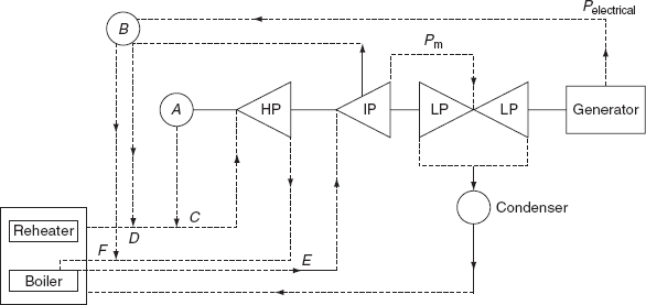
FIG. 12.12 Basic components of a reheat system unit
A is a primary governing system
B is an anticipatory governor system
C is the main governing valve or throttle blade
D is the combined stop and emergency valve
E is the interceptor governor valve
F is the combined stop and emergency valve
12.6.1.1 Primary Governing System
It responds to the speed of the main shaft. It controls either the main governor valve or throttle blades.
12.6.1.2 Secondary Governing System
The interceptor governing system will act as a secondary governing system and it responds to the frequency of turbines. It controls the interceptor valves between the HP stage and the reheater. It is usually set so that the interceptor valve is closed and it is about 25% to 50% open before the main governing valves commence to open. Consequently, this governing system is usually ignored.
12.6.1.3 Anticipatory Governing System
It responds to the accelerating power of the unit and it is usually not set to operate if either:
- The generator output is more than a certain value (i.e., 25% of maximum output) or
- The turbine mechanical power output (Pm) is less than a certain value (i.e., 80% of the maximum capacity).
For the activation of a governor, both these conditions should be violated.
This governing system is activated only when the unit suffers loss of a large percentage of its load and on sensing this condition, the emergency stop valves are closed very rapidly to prevent dangerous overspeed. The emergency stop valves are located very adjacent to the main governing valves.
A reset time delay is included so that when both electrical and mechanical powers revert to within settings, the emergency stop valves will open after a certain time.
This governing system is generally applied only on some modern large steam units.
12.6.1.4 Emergency Overspeed Governor Trip
When the shaft velocity exceeds a pre-set value, then this governor will close the combined stop and emergency valves and shut the set down. Starting up is a lengthy process, and usually this set would not figure any further in the stability calculations.
12.6.2 Block diagram representation
The block diagram representation of modeling a reheat system unit with a reduction in elements of Fig. 12.12 is shown in Fig. 12.13.
r = Steady-state droop system setting in rad/s/MW turbine power output
τg = Time constant of a governing system
R− = Maximum closing rate of a governing valve in MW/s

FIG. 12.13 Block diagram representation of modeling a simple reheat steam turbine unit
R+ = Maximum opening rate of the governing valve in MW/s
POSmax = Maximum power output of the turbine in MW (maximum governor valve opening)
POSmin = Minimum power output of the turbine in MW (governing valve may be closed)
τs = Equivalent time constant of steam entrained in the turbine HP stage
τrh = Equivalent time constant of the reheater and the associated piping
ωref = Reference speed setting of the governor in rad/s
ωshaft = Actual angular rotor velocity in rad/s
Delays and dead bands are present in the operations of:
- The speed-sensing mechanism, friction, and blacklash.
- Overcapping of oil ports in the servosystem as well as friction.
- Friction in the main governing valve.
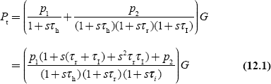
12.6.3 Transfer function of the steam-governor turbine modeling
Let |
GP1 |
= |
Power developed in the turbine at the HP stage |
|
τh |
= |
Time constant associated with entrained steam in the HP stage |
|
GP2 |
= |
Power developed in the subsequent stage of the turbine |
|
τr |
= |
Time constant associated with entrained steam in the reheater and connected pipe work |
|
τI |
= |
Time constant associated with entrained steam in IP and LP stages of the turbine. |
The expression for the turbine shaft power Pt as a function of the governor valve opening G is:
Since the reheater time constant is lower,
where C is the fraction of power developed in HP stage. The turbine power expression becomes
For representing a non-reheat system of turbine, simply replace τr by τI in Equation (12.3) and we get
12.7 MODELING OF A HYDRO-TURBINE-SPEED GOVERNOR
The block diagram representation of a simple, general hydro-turbine-speed-governor modeling is shown in Fig. 12.14.
r = Steady-state droop setting in rad/s/MW turbine output power
R = Transient droop setting in rad/s/MW turbine output power
τr = Recovery time constant of temperature droop dashpot
τg = Equivalent governor system time constant
R− = Maximum closing rate of the governor valve in MW/s
R+ = Maximum opening rate of the governor valve in MW/s
POSmax = Maximum power output of the turbine in MW (maximum governor valve opening)
POSmin = Minimum power output of the turbine in MW (usually the governor valve is fully closed)
The above modeling is based on some assumptions according to Kirchmayer:
- Neglecting dead band, delays, and non-linear performance in the governing system.
- Neglecting the variation in head of the set with daily use (or seasonal use).
- Assuming a constant equivalent water starting time constant.
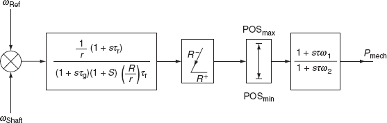
FIG. 12.14 Block diagram representation of a hydraulic turbine-speed governor
A transient droop setting ‘r’ and dashpot (i.e., damping) recovery time constant ‘τ’ are quite important in most stability studies, as the steady time is usually too short for the effective droop to reduce the steady-state value.
Representation of the water column inertia is important as there is an initial tendency for the turbine torque to change in the opposite direction to that finally produced when there is a change in the wicket gate in the case of a reaction turbine or an orifice opening in the case of an impulse turbine.
12.8 EXCITATION SYSTEMS
The excitation system consists of an exciter and an automatic voltage regulator (AVR). An exciter provides the required field current to the rotor winding of the alternator. The simplest form of an excitation system is an exciter only. When the task of the system becomes maintaining the constant terminal voltage of an alternator during variable load conditions, it incorporates the voltage regulator.
The voltage regulator senses the requirement from the terminal voltage of the alternator and actuates the exciter for the necessary increasing or decreasing of the voltage across the alternator field.
An excitation system with better reliabilities is preferable, even if the initial cost is more because of the fact that the cost of an excitation system is very small as compared to the cost of the alternator.
12.9 EFFECT OF VARYING EXCITATION OF A SYNCHRONOUS GENERATOR
Consider a synchronous generator supplying constant power to an infinite bus through a transmission line of reactance ‘X ’ Ω as shown in Fig. 12.15.
The output power of a synchronous generator is expressed as:
where |V| is the magnitude of terminal voltage, |I| the magnitude of current, and cos ϕ the p.f. It may be expressed in terms of torque angle δ as
where |E| is the magnitude of excitation voltage, |V| the magnitude of voltage at the bus, and δ the torque angle.
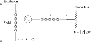
FIG. 12.15 Synchronous generator connected to an infinite bus
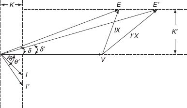
FIG. 12.16 Effect of varying excitation of a synchronous generator
The power output PG and voltage magnitude |V| at an infinite bus are constant; therefore, from Equations (12.4) and (12.5), we have
|I| cos ϕ = K (12.6)
|E| sin δ = K′ [∴ X is also a constant for this problem] (12.7)
where K and K′ are constants.
Equations (12.6) and (12.7) are clearly explained by the phasor diagram given in Fig. 12.16.
According to the phasor diagram shown in Fig. 12.16, for the variation of excitation, the tip of the excitation voltage vector ‘E’ is restricted to move along the horizontal dotted line, and the tip of the current vector ‘I’ is restricted to move along the vertical dotted line.
It is observed from Fig. 12.16 that when the excitation increases the torque angle ‘δ’ reduces (from δ to δ′), the current increases, and power angle increases from ϕ to ϕ′ and hence becomes more lagging with respect to the terminal voltage ‘V’.
Hence, the torque angle ‘δ’ is reduced with an increase in excitation, which results in an increase in stiffness of the machine, i.e., the couplings of the generator rotor and rotating armature flux become more tight. In other words, with the increase in excitation, the stability of the machine will become enhanced.
12.9.1 Explanation
For the increment in excitation voltage, the torque angle δ reduces.
Let us assume that a cylindrical rotor (wound rotor) synchronous generator connected to an infinite bus is initially operating at torque angle δ0 and supplying a power ![]() .
.
The generator output is equal to the turbine power, ![]() .
.
Now, draw the power angle characteristics of the generator as shown in Fig. 12.17(a).
We have the power output of the generator as:
For a stable region, ![]()
At δ = 90°, ![]() [∵ sinδ = 0]
[∵ sinδ = 0]
For an unstable region, ![]()
With the decrease in excitation, the torque angle increases, and hence the stiffness of the machine decreases.
From the power angle characteristics shown in Fig. 12.17(a), a graph between |E| and δ can be drawn as shown in Fig. 12.17(b).
It is observed that by decreasing the excitation, point D is reached and the instability will take place at ![]() . The occurrence of instability is shown as a drift in the curve. At any point on the lower portion of the curve, δ = f(|E|), the stable state is maintained since it corresponds to the point
. The occurrence of instability is shown as a drift in the curve. At any point on the lower portion of the curve, δ = f(|E|), the stable state is maintained since it corresponds to the point ![]() on PG = f(δ) curve.
on PG = f(δ) curve.

FIG. 12.17 (a) Power angle characteristics of a synchronous generator at different excitations; (b) the value of δ as a function of |E|
∴ The stability criterion of the system can be mathematically formulated as
And its critical point is given by ![]() .
.
Differentiating the above equation with respect to |E|, we get
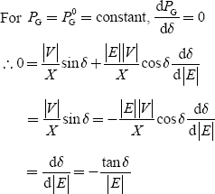
Instability will occur when δ → 90°,
![]()
From Fig. 12.17, it is concluded that the steady-state stability of the synchronous generator is improved by increasing its excitation.
12.9.2 limitations of increase in excitation
The increase in excitation is limited by the following factors:
- Maximum output voltage of the exciter supplying the field current.
- Resistance of the field circuit.
- Saturation of the magnetic circuit and rotor heating.
12.10 METHODS OF PROVIDING EXCITATION
The excitation is provided by the following two methods:
- Common excitation bus method.
- Individual excitation method
12.10.1 Common excitation bus method
It is also known as the centralized excitation method. In this method, two or more number of exciters feed a common bus, which supplies an excitation to the fields of all generators in the plant.
12.10.2 Individual excitation method
It is also known as the unit-exciter method. In this method, each generator is fed from its own exciter, which is usually direct connected to the generator shaft, but sometimes it is driven by a motor or a small prime mover or both.
The individual excitation (or) unit-exciter method is more preferable because a fault in any one exciter affects the entire excitation system.
12.10.2.1 Merits of individual excitation methods
- Simplicity: Since each alternator has its own exciter, this method of excitation results in a simple layout of the station. The exciters are so selected according to the requirement of individual generators that the main field rheostats and high-capacity switch gear are not required, which are necessary in the case of the common bus excitation method.
- Less ohmic losses: The ohmic losses are very less because no rheostats are required in the generator field circuit, and the exciter field rheostats are operated at a much lower power.
- Higher reliability: As any fault that occurs in exciter affects only the generator to which it is connected, the unit-exciter method has higher reliability than common exciter method.
- Incorporation automatic regulators: The AVRs are incorporated in an individual (or) unit excitation system for reliable sharing of reactive power to maintain constant terminal voltage while the generators are running in parallel.
- Less maintenance: Since the unit excitation system has no main field rheostats and high-capacity switchgear, the individual excitation system requires less maintenance and due to this it has less maintenance cost.
It is important to note that an excitation system with better reliability is preferred even though its initial cost is more because of the fact that the cost of an excitation system is very less as compared to the cost of a generator.
12.10.3 Block diagram representation of structure of a general excitation system
A block diagram representation of the structure of a general excitation system is shown in Fig. 12.18.
The main components present in the block diagram are:
12.10.3.1 Synchronous generator
It may be the type of high-speed turbo-alternator run by a steam turbine or a low-speed AC generator run by a hydro-turbine. With the help of an excitation system, the terminal voltage of an alternator or a synchronous generator should be maintained constant during variable load situations.
12.10.3.2 Exciter
It supplies the field current to the rotor field circuit of the synchronous generator. It may either be a self-excited type or separately exciter type of DC generator.
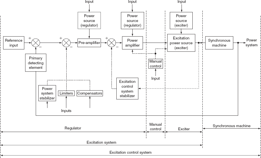
FIG. 12.18 Block diagram representation of a general excitation system

FIG. 12.19 Response of an exciter when separately excited and self-excited
In a self-excited exciter, a few turns are added for compounding and inter-poles are used. In separately excited exciters, an exciter field is supplied from a small DC generator known as the pilot exciter. A pilot exciter is a level compound generator and maintains constant voltage excitation for the main exciter.
The response of an exciter when compared to separately excited with that when self-excited is shown in Fig. 12.19.
Usually, the separately excited exciter, known as main exciter, is provided with two or more than two field windings, as shown in Fig. 12.20. Due to this arrangement of field, an easier automatic voltage regulation is permitted.
The voltage of the main exciter should be controlled from zero to ceiling voltage, the maximum voltage that may be attained by the exciter under specified conditions, to obtain rapid correction of exciter voltage after disturbance or fault. The faults or system disturbances cause an AVR to force an excitation up. After post-fault, rapid reduction of field is necessary to adjust the excitation to the correct value. This is easily achieved with a negative field. The main positive field is arranged in two parallel sections with rheostats for adjusting the field currents as required.
Hence, the positive and negative field windings of the main exciter with the adjustments of currents according to the load on the exciter maintain the exciter voltage and excitation as required.

FIG. 12.20 Exciter field arrangements
Due to the several parallel connected field windings, the fast response of the exciter is achieved, because of low time constant of the whole field circuit.
For small-sized turbo-generators, the exciters are usually directly coupled to the generator shaft. For medium-and large-sized turbo-generators, the exciters are coupled to the main shaft through the gear and are generally driven at 1,000 rpm.
For smaller generators (i.e., rated up to 25 MVA or so), self-excited exciters must be used and for large-sized generators of above 25 MVA, separately excited exciters are used. The exciter voltage of the main exciter is usually 230 V. In some cases, a nominal voltage of 440 V is used. The main exciter load in the resistance is the alternator field winding and this is generally between 0.25 and 1.0 Ω. The rotor current is about 10 A per MVA of alternator rating.
12.10.3.3 Use of amplidyne
In some cases, the DC excitation system is equipped with an amplidyne. An amplidyne provides large currents to the field winding of the main exciter.
It is a high-response cross-field generator and has a number of control windings, which can be supplied from the pilot exciter and a number of feedback circuits of an AVR and magnetic amplifier, etc. for control purposes. An amplidyne has a very high amplification factor of 106 or even more and needs very small control power.
12.10.3.4 AVR
An AVR in conjunction with the exciter tries to maintain constant terminal voltage of on an AC generator. The voltage regulator, in fact, couples the output variables of the synchronous generator to the input of the exciter through feedback and forwarding elements for the purpose of regulating the synchronous machine output variables. Thus, the voltage regulator may be assumed to consist of an error detector, pre-amplifier, power amplifier, stabilizers, compensators, auxiliary inputs, and limiters. The voltage regulator is treated as the heart of an excitation system. Exciter and regulator constitute an excitation system. Exciter, regulator, and synchronous generator constitute a system known as the excitation control system.
12.11 EXCITATION CONTROL SCHEME
A typical excitation control scheme is shown in Fig. 12.21.
The field winding of an alternator is connected to the exciter. The alternator terminal voltage is rectified by means of a potential transformer (PT) and rectifier, and is fed to a voltage regulator. A voltage regulator compares the rectified output voltage with a reference voltage Vref. The error signal output Ve = |Vref – Vdc | from the voltage regulator is amplified by an amplifier and the amplifier output voltage is fed to the exciter field winding.
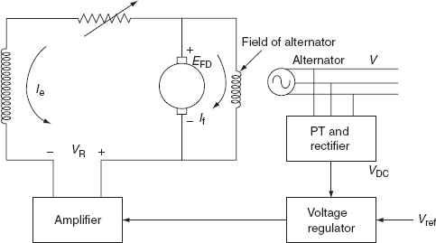
FIG. 12.21 A typical excitation control scheme
There is no error signal output from the regulator and the field winding current of exciter Ie is constant when the output voltage (terminal voltage) of an alternator is at a nominal value.
When the load on the alternator varies, the terminal voltage also varies. Hence, the error signal can be produced by the regulator, amplified, and fed to the field winding of the exciter. The field winding current of the exciter is varied and hence the terminal voltage reaches the required level.
12.12 EXCITATION SYSTEMS— CLASSIFICATION
The excitation systems are broadly classified into the following categories:
- DC excitation system.
- AC excitation system.
- Static excitation system.
12.12.1 DC excitation system
It consists of different configurations of rotating exciters like:
- Self-excited exciter with a direct-acting rheostatic-type voltage regulator.
- Main and pilot exciters with an indirect-acting rheostatic-type voltage regulator.
- Main exciter, amplidyne, and static voltage regulator.
- Main exciter, magnetic amplifier, and static voltage regulator.
The main drawbacks of a DC excitation system are:
- Complexity is more due to rotating exciters, voltage regulators, and moving contacts like slip rings and brushes.
- Time constants of exciter, voltage regulator, amplidyne, and magnetic amplifier are large (about 3 s).
- Difficulties of commutation.
- Smoothless operation needs continuous maintenance.
- Reliability is less.
- Noise level is more due to rotating exciters.
12.12.2 AC excitation system
It consists of an AC generator and a thyristor (rectifier) bridge circuit directly connected to the alternator shaft. The main advantage of this method of excitation is that the moving contacts such as slip rings and brushes are completely eliminated thus offering smooth and maintenance-free operation. Such a system is known as a brushless excitation system. In this system, there are no commutation problems.
12.12.3 Static excitation system
It consists of a step-down transformer and a rectifier system using mercury arc rectifiers of silicon-controlled rectifiers (SCRs). The rotating amplifiers and rotating exciters are replaced by the static devices of a rectifier system.
The advantages of a static excitation system are:
- Noise-free operation in the plant is obtained as the rotating exciters are replaced with static devices of rectifiers.
- Since the static excitation equipment may be mounted or placed separately at a convenient place, the complexity of the excitation system is reduced.
- Due to static devices, the overall length of the generator shaft is reduced, which simplifies the torsion problem and the problem of critical speed. The generator rotor is easily withdrawn for maintenance purpose.
- High reliability compared to other excitation systems because of having more reliable static devices and
- Static devices are provided with low-speed hydro-alternators, where large-sized rotating exciters are needed.
12.13 VARIOUS COMPONENTS AND THEIR TRANSFER FUNCTIONS OF EXCITATION SYSTEMS
In this section, we shall discuss PT and rectifier, voltage comparators, and amplifiers in detail.
12.13.1 PT and rectifier
One possible arrangement of a PT and a rectifier is shown in Fig. 12.22. The terminal voltage of the alternator is stepped down by the PT and rectified to form VDC, which is proportional to the average RMS value of the terminal voltage Vt.

FIG. 12.22 Connections of PT and rectifier
Transfer function of the arrangement is represented as:
where KR is the proportionality constant (or) gain of the PT and rectifier assembly and τR the time constant of the assembly due to filtering in the assembly arrangement.
12.13.2 Voltage Comparator
A voltage comparator compares the rectified DC voltage of the generator with a reference voltage Vref and produces an output in the form of an error signal Ve. Figure 12.23 shows an electronic difference amplifier as a comparator.
The output voltage or an error voltage Ve is expressed as
Ve(S) = K(Vref(S) – Vdc(S))
12.13.3 Amplifiers
Among the various types of amplifiers used in an excitation system, the amplidyne and magnetic amplifier have high amplification factors.
12.13.3.1 Amplidyne
Basically, a cross-field DC generator is operated as an amplidyne. An amplidyne configuration is shown in Fig. 12.24.
The operation of an amplidyne consists of two stages of amplification.
First Stage of Amplification
An amplidyne consists of brushes along the d-axis and the q-axis. The brushes along the q-axis are short-circuited. As the armature resistance is very small, a small amount of field m.m.f. results in a large q-axis current. This production of the large q-axis current is treated as the first stage of amplification.
Second Stage of Amplification
The large q-axis current produces a flux in time and space phase with itself. Corresponding to this q-axis flux, the voltage will be developed across the d-axis brushes. The development of voltage across d-axis brushes due to the q-axis current is termed as the second stage of amplification.
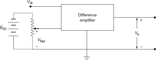
FIG. 12.23 Electronic difference amplifier as a comparator

FIG. 12.24 Amplidyne configuration
The d-axis brushes are connected to the load along with a compensating winding, which provides no resultant excitation due to load current since it may reduce the original field excitation. (It has a number of control windings supplied from the pilot exciter and has a number of feedback circuits of AVR and magnetic amplifier, etc. for control purposes.)
The advantages of the second stage of amplification are as follows:
- Power required for control purpose is very small.
- As the response time is very less, it has a fast response.
- Amplification factor is of 106 or even more.
The transfer function of an amblidyne under no-load condition can be expressed as
where τa is the time constant of armature, τr the time constant of field, and KA the voltage amplification factor.
12.13.3.2 Magnetic amplifier
Magnetic amplifier configuration is shown is Fig. 12.25. It consists of a saturable core, control winding, and a rectifier circuit.
The saturable core reactor can be designed so that when no DC current is flowing through the DC control winding, the inductive reactance of AC coils is very high and limits the flow of AC current to a small value.
In a magnetic amplifier when large DC current flows through the control winding, the core gets saturated. This results in the decrement in permeability and hence the reactance of AC coils decreases. Therefore, more AC current flows. This AC current is rectified and fed to the load.

FIG. 12.25 Configuration of a magnetic amplifier
The controlling of a large output current by means of a small control current is the main principle of a magnetic amplifier.
The transfer function of a magnetic amplifier can be expressed as
where Ve is an error signal input applied to control winding, VR is the output voltage and is governed by the limits, i.e., VR min ≤ VR ≤ VR max, KA is the amplification factor, and τA is the time constant amplifier.
12.14 SELF-EXCITED EXCITER AND AMPLIDYNE
The amplidyne is connected in series with the shunt field of the main exciter as shown in Fig. 12.26.
Let VR be the armature emf of the amplidyne,
efd the armature emf of main exciter,
Ne the number of field turns of main exciter under no-load condition,
ϕe the flux of the main exciter under no-load condition,
re the field circuit resistance of the exciter under no-load condition, and
ie the field current of the exciter under no-load condition.

FIG. 12.26 Circuit diagram of series combination of an amplidyne with the shunt field of the main exciter
For an exciter field circuit,
Since efd is a function of ϕe, effective flux of the main exciter
where ![]() , a constant for the armature
, a constant for the armature
Difference of ϕfe and ϕe is an account of leakages flux ϕl, proportional to field current ie, and may be written as
ϕfe = ϕe + ϕ1
and ϕ1 = C1ϕe
where C1 is the proportionality constant:
ϕfe = ϕe + C1ϕe
= (1 + C1) ϕe
ϕfe = σϕe
where σ is known as the coefficient of dispersion having a value in the range of 1.1–1.2.

where τE is known as time constant of the exciter.
However, the effect of saturation of the exciter voltage efd is taken into account while solving the above equation.
The exciter characteristics are shown in Fig. 12.27.
It is evident that the saturation of the exciter SE is a non-linear function of the exciter voltage efd and is given as

FIG. 12.27 Exciter characteristics
From the above, we can write ![]()
If the slope of the air-gap line is ![]()
![]()
or ie = G (1 + SE) efd
Substituting ie in equation ![]() we have
we have
![]()
Taking Laplace transform of the above equation, we get
VR(S) Efd(S) = reG(1 + SE)Efd(S) + sτBEfd(S)
From the above, we can get
![]()
where KE = reG−1
12.15 DEVELOPMENT OF EXCITATION SYSTEM BLOCK DIAGRAM
The simplified diagram of an excitation system with fundamental components is as shown in Fig. 12.28.

FIG. 12.28 Simplified diagram of a buck-boost excitation system
For the complete analysis of the excitation system, it is necessary to develop the transfer function of each component and then the transfer function of an overall excitation system.
Transfer function of PT and rectifier is
Transfer function of an amplifier is
Transfer function of the exciter is
Here, ![]()
If the saturation is neglected i.e., SE = 0,
∴ Transfer function of the exciter can be written as
12.15.1 Transfer function of the stabilizing transformer
An equivalent circuit of a stabilizing transformer is shown in Fig. 12.29.
The excitation system that was described earlier has a dynamic response that is prone to excessive overshoot and stability problems. These problems are overcome by adding a stabilizing transformer. For the stabilizing transformer, the input becomes Efd and the output is VST.

FIG. 12.29 Equivalent circuit of a stabilizing transformer
The output VST is subtracted from V, i.e., V − VST to provide the input to the amplifier:
Input, ![]()
In Laplace transform,
Efd(s) = (R1 + sL1) I1(s)
and output ![]()
i.e., VST(s) = sMI1(s)
∴ Transfer function of a stabilizing transformer is
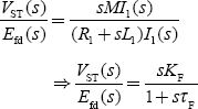
where ![]() = Transformer gain
= Transformer gain
and ![]() = Transformer time constant.
= Transformer time constant.
12.15.2 Transfer function of synchronous generator
where KG is the gain of the generator and τG the time constant of a rotor field.
12.15.3 IEEE type-1 excitation system
Most of the excitation systems are modeled based on IEEE type-1 excitation system, which was produced by the report of the first IEEE committee in 1968. The complete block diagram of an IEEE type-1 excitation system is as shown in Fig. 12.30 by interconnecting all the components in the forward path and the feedback control loop.

FIG. 12.30 IEEE type-1 excitation system
|
EFD |
= |
Exciter output voltage (applied to generator field) |
|
IFD |
= |
Generator field current |
|
IT |
= |
Generator field terminal current |
|
KA |
= |
Regulator gain |
|
KE |
= |
Exciter constant related to self-excited field |
|
KF |
= |
Exciter saturation function |
|
τA |
= |
Regulator amplifier time constant |
|
τE |
= |
Exciter time constant |
|
τF |
= |
Regulated stabilizing circuit time constant (τF1 and τF2) |
|
τR |
= |
Regulated input filter time constant |
|
VR |
= |
Regulator output voltage |
|
Vt |
= |
Terminal voltage of the generator applied to the regulator input |
|
KG |
= |
Gain of the generator |
|
τG |
= |
Time constant of the generator rotor field |
When the generator is operating at an equilibrium state, i.e., at rated voltage, the voltage of the rotating amplifier VR becomes zero. If the generator load is increased such that the sensing circuit shown in Fig. 12.30 detects this fall in terminal voltage, it causes the amplidyne to increase the field current Ie in the exciter field. Hence, the exciter voltage increases and in turn increases the generator field current If that ultimately should rise the terminal voltage of generator, Vt.
Under steady-state conditions, E = Efd.
Under transient conditions, any mismatch between E and Efd will cause the voltage ![]() to change after some delay.
to change after some delay.
Mathematically, ![]()
where ![]() is the open-circuit generator, direct axis transient time constant.
is the open-circuit generator, direct axis transient time constant.
12.15.4 Transfer Function of Overall Excitation System
The transfer function of an overall excitation system, shown in Fig. 12.31, can be obtained by either using the block diagram reduction technique or the signal flow graph method.
First, neglect the effect of saturation:
i.e., SE = 0
and remove the stabilizing transformer from the block diagram shown in Fig. 12.30.
∴ The transfer function of the system is of the form:

where ![]() and is known as the feed-forward transfer function and
and is known as the feed-forward transfer function and ![]() is known as the feedback transfer function.
is known as the feedback transfer function.
∴ The transfer function of the excitation system is expressed as
In the transfer function ![]() , τR is a simple time constant representing regulator input filtering. It is very small and may be considered to be zero for many systems.
, τR is a simple time constant representing regulator input filtering. It is very small and may be considered to be zero for many systems.
The first summing point compares the regulator reference with the output of the input filter to determine the voltage error input to the regulator amplifier.
The AVR usually comprises several control loops and a simple reduction is necessary to the form ![]() . Voltage regulator gain (KA) has an important effect on power system performance while the time constant τA has a much smaller influence owing to large τe in series.
. Voltage regulator gain (KA) has an important effect on power system performance while the time constant τA has a much smaller influence owing to large τe in series.
Because of high gain in an excitation system (100–400), errors in forward-path gain KA are more important than errors in most other parameters (including generator and network).
The second summing point combines the voltage error input with the excitation damping loop signal. KA and τA represent the main regulator gain and its transfer function. The minimum and maximum limits of the regulator are imposed so that large input error signals may not produce a negative output, which exceeds the practical limit.
The next summing point subtracts a signal that represents the saturation function SE = f (EFD) of the exciter. That is, the exciter output voltage (or generator field voltage EFD) is multiplied by a non-linear saturation function and subtracted from the regulator output signal. The resultant is applied to the exciter transfer function ![]() .
.
Major loop damping is provided by the feedback transfer function, ![]() from the exciter output EFD to the first summing point.
from the exciter output EFD to the first summing point.
If the stabilizing loop is omitted, the exciter system and the main generator will be unstable for most practical values of KA. It can only be omitted when there are additional input signals to the excitation system such as frequency derivatives, etc.
The useful value of KF is from 0.1 to 0.15 and τF varies in the range 0.5 –2.0 s.
Vref = Regulator reference voltage setting
VRH = Field rheostat setting
VT = Generator terminal voltage
ΔVT = Generator terminal voltage error
Note that there is an interrelation between the exciter ceiling voltage EFDmax, regulator ceiling ERmax, exciter saturation, SE and KE.
Under steady-state condition,
VR – (KE + SE) EFD = 0; EFDmin ≤ EFD ≤ EFDmax
At the ceiling or EFD α EFDmax, the above equation becomes
VRmax − (KE + SEmax)EFDmax = 0
The exciter saturation function is defined as the multiplier of the exciter output EFD to represent the increase in exciter excitation requirement because of saturation.
The exciter time constant τe is a dominant time constant in the excitation system. If it is not possible to obtain data for the main exciter saturation function, then a useful approximation is to increase τe by 20% and decrease the exciter ceiling voltage by 20%.
12.16 GENERAL FUNCTIONAL BLOCK DIAGRAM OF AN EXCITATION SYSTEM
The general functional block diagram of an excitation system is shown in Fig. 12.31.
12.16.1 Terminal voltage transducer and load compensation
The terminal voltage of the alternator is sensed and rectified into a DC voltage by means of a terminal voltage transducer.
The load compensation synthesizes a voltage, which differs from the terminal voltage by the voltage drop in an impedance (RLC + jXLC). Both voltage and current phasors must be used in computing the compensating voltage VC.
12.16.1.1 Objectives of load compensation
- Sharing of reactive power among the units, which are bussed together with zero impedance between them. For this, RLC and XLC are positive and the voltage is regulated at a point internal to the generator.
- When the units are operating in parallel through unit transformers, it is desirable to regulate voltage at a point beyond the machine terminals to compensate for a portion of transformer impedance. For this case, both RLC and XLC are negative values. RLC is neglected in most of the cases.
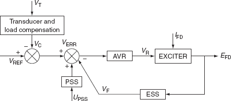
FIG. 12.31 Functional block diagram of an excitation control system
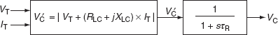
FIG. 12.32 Modeling of transducer and load compensation
The modeling of terminal voltage transducers and load compensation is as shown in Fig. 12.32.
The voltage transducer is usually modeled as a single time constant τR and it is very small and assumed to be zero for simplicity in many cases.
12.16.2 Exciters and voltage regulators
The AVRs of modern type are continuously acting electronic regulators with high gain and lower time constants.
12.16.2.1 Types of exciters
The types of exciters are shown in Fig. 12.33(a). The block diagram representation of an exciter and a regulator is shown in Fig. 12.33(b).
In Fig. 12.33(b), VR is the output of the regulator, which is limited:
τA — single time constant of regulator
KA — positive gain
Saturation function SE = f (EFD) represents the saturation of the exciter.
Note: The limits on VR can be found from steady-state equation:
VR – (KE + SE) ERD = 0
This implies limits on EFD such that:
EFDmin ≤ EFD ≤ EFDmax
With the specification of parameters, KE = 1, τE = 0, SE = 0, and VRmax = KpVT, IEEE type-1 system represents the static excitation system with potential source-controlled rectifier type.
12.16.3 Excitation system stabilizer and transient gain reduction
This system is used to increase the stability region of operation of the excitation system and also permit higher regulator gains.
The feedback transfer function of the ESS is shown in Fig. 12.34.
The ESS is realized by an ideal transformer whose secondary is connected to high impedance as shown in Fig. 12.35.
The turns ratio of the transformer (n) and the time constant of the circuit ![]() determine KF and τF such as
determine KF and τF such as ![]() and
and ![]()
τF is usually 1 s.
A series-connected load or lag circuit can also be used instead of feedback compensation circuit for ESS as shown in Fig. 12.36.
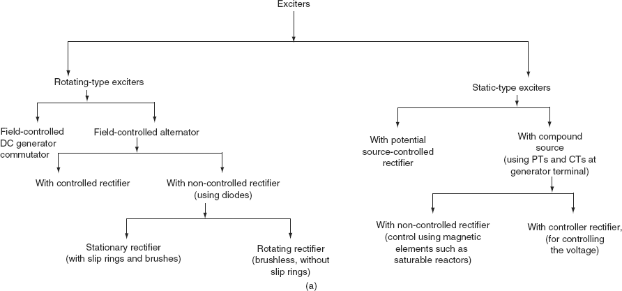
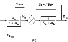
FIG. 12.33 (a) Classification of exciters; (b) block diagram representation of exciter and voltage regulator
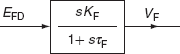
FIG. 12.34 ESS transfer function
FIG. 12.35 Realization of ESS

FIG. 12.36 TGR
Here, τC > τB and stabilization is termed as TGR. Reducing the transient gain (or gain at higher frequencies), thereby minimizing the negative contribution of the regulator to system damping, is the main objective of TGR. The TGR may not be required, if power system stabilizer (PSS) is specifically used to enhance system damping.
Usually, TGR factor ![]()
12.16.4 Power system stabilizer
During the transient disturbance, the rotor oscillations of frequency 0.2–2.0 Hz are damped out by providing the PSSs. The damping of rotor oscillatations can be impaired by the provision of high-gain AVR, particularly at high loading conditions when a generator is connected through a high external impedance (due to weak transmission network).
The input signal to PSS is derived from speed or frequency or accelerating power or a combination of these signals.
The output of PSS, VS, is added to the terminal voltage error signal.
12.17 STANDARD BLOCK DIAGRAM REPRESENTATIONS OF DIFFERENT EXCITATION SYSTEMS
The standard block diagrams of different excitation systems based on supply were published by the second IEEE committee report in the year 1981.
12.17.1 DC excitation system
Figure 12.37 shows the type DC-1 excitation system. It consists of a DC commutator exciter with a continuously acting voltage regulator. This is similar to the IEEE type-1 excitation system.
The TGR can be represented by the transfer function ![]() with τB > τC. It has the similar function as ESS in the feedback path.
with τB > τC. It has the similar function as ESS in the feedback path.
Either TGR in the forward path or ESS in the feedback path is shown in the block diagram representation.
With τB = τC, the TGR can be avoided and similarly with KF = 0, ESS can be neglected.
12.17.1.1 Derivation of transfer function
(i) For separately excited DC generator (exciter)
Figure 12.38 shows the separately excited DC generator. From Fig. 12.38,
The generator (exciter) output voltage Eg is a non-linear function of If as shown in Fig. 12.39.

FIG. 12.37 Type DC 1-DC commutator exciter

FIG. 12.38 Separately excited DC generator

FIG. 12.39 Exciter load saturation curve
Assume the speed of the exciter to be constant. From Fig. 12.39, we have the following:

where Rg is the slope of the saturation curve near Eg = 0. Express If in p.u. of Ifb:
where Egb is the rated voltage that is defined as the voltage, which produces rated open-circuit voltage in the generator-neglecting saturation:

where S′E = RgSe
The block diagram of a separately excited generator is shown in Fig. 12.40.
(ii) Self-excited DC generators
The schematic diagram of a self-excited exciter is shown in Fig. 12.41.
Ea represents the voltage of the amplifier in series with the exciter shunt field.

FIG. 12.40 Block diagram of a separately excited DC generator

FIG. 12.41 Schematic diagram of a self-excited exciter
The block diagram of Fig. 12.41 with Ea = VR can be reduced such that ![]()
The Rf is periodically adjusted to maintain VR = 0 in the steady state, for this KE = –SEo where SEo is the value of saturation function SE at the initial operating point and KE is generally negative for a self-excited exciter.
12.17.2 AC excitation system
The block diagram of a type AC-1 excitation system is shown in Fig. 12.42. This represents the field-controlled alternator rectifier with non-controlled rectifier-type AC excitation system.
The term KD IFD represents armature reaction of the alternator and FEX represents rectifier regulation.
Constant KD is a function of the synchronous alternator, and transient reactance constant KC is a function of the commutating reactance.
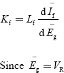
The function FBX is given as
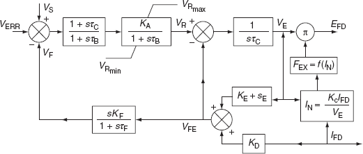
FIG. 12.42 Block diagram of type AC-1 excitation system
The signal VFE is proportional to the exciter field current and is used as an input to ESS.
12.17.3 Static excitation system
There are two types of static excitation systems:
- With a potential source-controlled rectifier—In this, the excitation power is supplied through a PT connected to generator terminals.
- With a compound source-controlled rectifier—In this, both current transformer (CT) and PT are used at generator terminals.
The block diagram of the potential source-controlled rectifier excitation system is shown in Fig. 12.43.
In this block diagram, the internal limiter following the summing junction can be neglected, but field voltage limits that are dependent on both VT and IFD must be considered.
For transformer-fed systems, KC is small and can be neglected.
In these systems, transformers are used to convert voltage (and also current in compounded systems) to the required level of field voltage with the aid of controlled or uncontrolled rectifiers. As the exciter ceiling voltage tends to be high in static exciters, field current limiters are used to protect the exciter and field circuit.
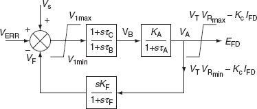
FIG. 12.43 Block diagram-type ST1-potential source-controlled rectifier excitation system
KEY NOTES
- According to the control, speed-governing systems are classified as:
- Mechanical-hydraulic-controlled.
- Electro–hydraulic-controlled.
- The significance of rate and position limits in a speed-governing system are:
- Rate limiting of servomotor may occur for large, rapid-speed deviations, and rate limits are shown at the input to the integrator.
- Position limits are indicated that correspond to wide-open valves or the setting of a load limiter.
- For wind-up limiter, the output variable of the transfer function G(s) is not limited and is free to vary. Hence, the wind-up can be treated as a separate block in the modeling of a speed-governing system.
- For non-wind-up limiter, the output variable of the transfer function G(s) is limited and there is no separate block in the modeling of a speed-governing system.
- Secondary governing system responds to the frequency of turbines and it controls the interceptor valves between the HP state and the reheater.
- Exciter provides the required field current to the rotor winding of a synchronous generator. It may either be self-excited type or separately excited type.
- In the unit excitation method, each generator is fed from its exciter, which is usually directly connected to the generator shaft.
- Amplidyne is a high-response cross-field generator, which has a number of control windings that can be supplied from a pilot exciter and a number of feedback circuits of AVR and magnetic amplifier for control purposes.
- An AC excitation system consists of an AC generator and a thyristor bridge circuit directly connected to the generator shaft
- By providing PSS, the rotor oscillations are damped out during the transient disturbance.
SHORT QUESTIONS AND ANSWERS
- What is the classification of speed-governing systems according to the control?
- Mechanical-hydraulic-controlled.
- Electro-hydraulic-controlled.
- What is the function of hydraulic servomotors used in mechanical-hydraulic-controlled and electro– hydraulic-controlled speed-governing systems?
For positioning valve or gate controlling system or water flow.
- What are the components of mechanical-hydraulic-controlled speed-governing systems used for steam turbines?
Speed governor, speed relay, hydraulic servomotor, and speed-governor-controlled systems.
- Why do the electro-hydraulic-controlled speed-governing systems provide more flexibility than mechanical-hydraulic-controlled speed-governing systems?
In electro-hydraulic-controlled speed-governing systems, mechanical components in the lower power portions are replaced by the static electronic circuits.
- How does the linearity of electro-hydraulic-controlled speed-governing systems improve?
By providing feedback loop of steam flow and the servomotor.
- What are the components of mechanical-hydraulic-controlled speed-governing systems for hydro-turbines?
A speed governor, a pilot valve, and servomotor, a distributor valve and gate servomotor, and governor-controlled gates.
- What is required to achieve the stable performance of speed-governing system for hydro-turbines?
Dashpot feedback is required to achieve the stable performance of speed-governing system for hydro-turbines.
- How is the speed relay represented in the approximate non-linear modeling of a speed-governing system?
As an integrator and provided as a direct feedback.
- How is the non-linear property of the speed-governing valve compensated?
By providing a non-linear CAM in between the speed relay and the hydraulic servomotor.
- What is the significance of a servomotor in the speed-governing system?
The servomotor controls the movements of valves and it is represented as an integrator with time constant τsm and it provides as direct feedback.
- What is the significance of rate limits and position limits in approximate non-linear modeling of a speed-governing system?
- Rate limiting of servomotor may occur for large, rapid-speed deviations, and rate limits are shown at the input to the integrator.
- Position limits are indicated as there corresponding to wide-open valves or the setting of a load limiter.
- What do you mean by wind-up limiter and non-wind-up limiter?
In the case of a wind-up limiter, the output variable of the transfer function G(s) is not limited and is free to vary. Hence, the wind-up can be treated as a separate block in the modeling of a speed-governing system.
In the case of a non-wind-up limiter, the output variable of the transfer function G(s) is limited and there is no separate block in the modeling of the speed-governing system.
- When modeling steam-turbine generators, which equipment is to be ignored at every instant?
The boiler controls and on-line frequency control equipment should be ignored at every instant due to their slower operations.
- What are the parts of a speed-governing system in a reheat system unit?
Primary governing system, secondary governing system, and anticipatory governing system are the parts of a speed-governing system.
- What is the primary governing system of a reheat system unit?
Primary governing system responds to the speed of a main shaft. It controls the main governor valve or throttle blades.
- What is the secondary governing system of a reheat system unit?
Secondary governing system responds to the frequency of turbines and it controls the interceptor valves between the HP state and the reheater. The interceptor governing system will act as the secondary governing system.
- What is anticipatory governing system of a reheat system unit?
An anticipatory governing system responds to the accelerating power and is usually not set to operate if either the generator output is more than a certain value (25% of maximum output) or the turbine mechanical power output is less than a certain value (i.e., 80% of maximum capacity).
- When will the anticipatory governing system be activated?
Only when the reheat system unit suffers loss of a large percentage of its load and on serving this condition, the emergency stop valves are closed very rapidly to prevent dangerous overspeeds.
- When will the emergency overspeed governor trip?
When the velocity of shaft exceeds a pre-set value, then emergency overspeed governor will close the combined stop and emergency valves and shut the set down.
- On what assumptions is the modeling of a hydro-turbine based?
According to Kirchmayer, the modeling of single, general hydro-turbines is based on the following assumptions:
- Neglecting dead band, delays and non-linear performance in the governing systems.
- Neglecting the variations in head of the set of hydro-turbine unit with daily use or seasonal use.
- Assuming a constant equipment water starting time (τw).
- What is the function of an exciter in an excitation system?
It provides the required field current to the rotor winding of a synchronous generator. It may be either self-excited type or separately excited type.
- What are the effects of increase in excitation?
- The torque angle δ reduces and
- The current increases and the power angle also increases and hence becomes more lagging with respect to terminal voltage.
- What is the effect of increase in excitation on stability of the synchronous machine?
When the excitation increases, the torque angle δ reduces, which results in an increase in stiffness of the machine. In other words, with an increase in excitation, the stability of the machine will improve.
- What are the factors by which the increase in excitation is limited?
- Maximum output voltage of the exciter.
- Resistance of the field current.
- Saturation of the magnetic circuit.
- Rotor heating.
- What are the methods of providing excitation?
- Common or centralized excitation method.
- Individual or unit excitation method.
- What do you mean by individual or unit excitation method?
In individual or unit excitation method, each generator is fed from its own exciter, which is usually directly connected to the generator shaft.
- What is the meaning of common or centralized excitation method?
In common or centralized excitation method, two or more number of exciters feed a common bus, which supplies excitation to the fields of all generators in the plant.
- Which method of providing excitation is more preferable?
Unit exciter or common excitation method is more preferable.
- What are the merits of individual or unit excitation method?
Simplicity, less ohmic losses, higher reliability, less maintenance, and the possibility of incorporation of automatic regulators.
- Why are automatic regulators incorporated in individual or unit excitation method?
For the reliable sharing of reactive power to maintain constant terminal voltage while generators are running in parallel.
- What is pilot exciter?
In separately excited-type exciters, exciter field is supplied from a small DC generator known as a pilot exciter, which is a level compound generator and maintains constant voltage excitation for the main exciter.
- What is the use of an amplidyne in a DC excitation system?
An amplidyne provides large currents to the field winding of a main exciter.
- What is an amplidyne?
Amplidyne is high-response cross-field generator, which has a number of control windings that can be supplied from pilot exciter and a number of feedback circuits of an AVR and a magnetic amplifier for control purposes.
- What is an AVR? What are its components?
The AVR in conjunction with the excitation tries to maintain a constant terminal voltage of a synchronous generator. It consists of an error detector, pre-amplifier, power amplifier, stabilizer, compensators, auxiliary inputs, and limiters.
- Which is treated as the heart of an excited system?
The heart of an excitation system is the AVR.
- What is an excitation control system?
An exciter, voltage regulator, and synchronous generator constitute a system known as an excitation control system.
- What are the classifications of excitation systems?
- DC excitation system.
- AC excitation system.
- Static excitation system.
- What are the drawbacks of a DC excited system?
- More complexity.
- Larger time constants of an exciter, voltage regulator and amplidyne, and magnetic amplifier.
- Difficulties of commutation.
- Smoothless operation.
- Less reliability.
- More noise level due to rotating exciter.
- What is an AC excitation system?
An AC excitation system consists of an AC generator and a thyristor bridge circuit directly connected to the generator shaft.
- What are the merits of an AC excitation system?
- Moving contacts are completely eliminated.
- Offering smooth and maintenance-free operation.
- There are no commutation problems.
- Which system of excitation is brushless excitation?
An AC excitation system is a brushless excitation system.
- What are the merits of static excitation systems?
- Noise-free operation.
- Less complexity.
- High reliability compared to other excitation systems.
- The overall length of the generator shaft is reduced, which simplifies torsion problem and critical speed operation.
- Write the transfer function of a potential transformer and rectifier of an excitation system.

where Kr is the gain of PT and rectifier assembly
τr is the time constant of the assembly
- What are the stages of operation of an amplidyne?
First stage of amplification and second stage of amplification are the stages of operation of an amplidyne.
- What is the first stage of amplification for the operation of an amplidyne?
An amplidyne consists of brushes along the q-axis and the d-axis. The brushes along the q-axis are short-circuited. As the armature resistance is small, a small amount of field m.m.f. results in a large q-axis current. This is the first stage of amplification.
- What is the second stage of amplification of operation of an amplidyne?
The development of voltage across d-axis brushes due to q-axis current is termed as the second stage of amplification.
- Write the transfer function of an amplidyne under no-load condition.

where τa is the time constant of the armature, τf the time constant of field, and KA the voltage amplification factor.
- What are the components of a magnetic amplifier?
A saturable core, control winding, and a rectifier circuit are the components of a magnetic amplifier.
- What is the main principle of a magnetic amplifier?
The controlling of a large output current by means of small control current is the main principle of a magnetic amplifier.
- Write the transfer function of a magnetic amplifier.

where τA is the time constant of the magnetic amplifier, Vr the output voltage, KA the voltage amplification factor, and Ve the error signal input.
- Write the transfer function of an exciter.

where τE is the time constant of the exciter, KE the gain of the exciter, VE the armature emf of an amplidyne, Efd the armature emf of the main exciter.
- What is the function of a stabilizing transformer?
The excitation system has dynamic response which is prone to excessive overshoot and stability problems. These problems are overcome by adding a stabilizing transformer to the excitation system.
- What is the function of a terminal voltage transducer represented in a functional block diagram of an excitation system?
The terminal voltage of the alternator is sensed and rectified into a proportionate DC signal by using a terminal voltage transducer.
- What is the function of load compensation block in an excitation system block diagram?
Load compensation synthesizes a voltage that differs from the terminal voltage by the voltage drop in the impedance.
- What is the significance of a saturation function SE, which is represented in an excitation system functional block diagram?
The saturation function SE = f(Efd) represents the saturation of the exciter.
- What are the main classifications of an exciter?
Rotating-type and static-type exciters are the main classifications of an exciter.
- What is the function of an excitation system stabilizer transient gain regulator block?
To increase the stability region of operation of the excitation system and also to permit a higher regulating gain.
- How is the excitation system stabilizer realized?
An excitation system stabilizer is realized by an ideal transformer whose secondary is connected to a high impedance.
- What is the function of PSS?
During the transient disturbance, the rotor oscillations (of frequency 0.2–2 Hz) are damped out by providing the PSS.
- What is a potential source-controlled-type static excitations system?
In a potential source-controlled-type static excitations system, the excitation power specified is supplied through a PT connected to generator terminals.
- What is a static excitation system with a compound source-controlled rectifier?
The excitation power is supplied through both CTs and PTs connected to generator terminals.
- What is the input signal to PSS?
The input signal to PSS is derived from speed or frequency or oscillating power or a combination of these signals.
MULTIPLE-CHOICE QUESTIONS
- Hydraulic servomotors are used in __________ type of speed-governing systems.
- Mechanical-hydraulic-controlled.
- Electro-hydraulic-controlled.
- Either (a) or (b).
- Both (a) and (b).
- In hydraulic-controlled speed-governing systems, the hydraulic servomotors are used for:
- Positioning the valve or gate, controlling steam or water flow.
- Removing the valve or gate, controlling steam or water flow.
- Improving the water head.
- Improving the steam pressure and temperature.
- For a steam turbine, the mechanical-hydraulic-controlled speed-governing system consists of which of the following?
- A speed governor.
- A speed relay.
- A hydraulic servomotor.
- Governor-controlled valves
- (i) and (iv)
- (iii) and (iv)
- All except (ii)
- All of these.
- In the approximate non-linear mathematical model of a mechanical-hydraulic-controlled speed-governing system, the term KG represents the gain of speed-governor system, which is ___________.
- The regulation or droop of characteristics.
- The reciprocal of regulation or droop of characteristics.
- Not the function of regulation or droop.
- None of these.
- The gain of a speed-governor KG represents:
- A position of an assumed linear instantaneous indication of a speed produced by the speed governor.
- The regulation or droop of speed-governor characteristics.
- The governor speed-changer position.
- None of these.
- The governor speed-changer position provides the relay signal and is determined by:
- A system of speed governing.
- A system of automatic generation control.
- A system of hydraulic servomotor control.
- None of these.
- The speed relay signal in mechanical-hydraulic speed-governing system represents a composite load and speed reference and is assumed ___________ over the interval of a stability study.
- The speed relay in a mechanical-hydraulic speed-governing system is represented as:
- An integrator.
- A differentiator.
- An amplifier.
- None of these.
- The speed relay in a mechanical-hydraulic speed-governing system provides:
- An indirect feedback.
- A direct feedback.
- No feedback.
- None of these.
- The non-linearity property of the valve is compensated by means of providing:
- A linear CAM.
- A non-linear CAM.
- A speed relay.
- A hydraulic servomotor.
- A non-linear CAM is provided to compensate the non-linear property of the valve in between:
- The hydraulic servomotor and governor-controlled valve.
- The speed governor and the speed relay.
- The speed relay and the hydraulic servomotor.
- The hydraulic servomotor and the speed governor.
- The hydraulic servomotor:
- Controls the moments of valves.
- Is represented as an integrator in the approximate linear model.
- For which the rate timing may occur for large-and rapid-speed deviations.
- All of these.
- The hydraulic servomotor control provides:
- A direct feedback.
- An indirect feedback.
- No feedback.
- None of these.
- The position limits of the hydraulic servomotor that are indicated correspond to:
- Wide-open valves.
- The setting of a load limiter.
- Either (a) or (b).
- None of these.
- The non-linearities present in speed control mechanism are not neglected for:
- Rate limits of servomotor.
- Position limits of valve.
- Study of power system components.
- Both (a) and (b).
- The mechanical components in the lower power portions are replaced by the static electronic circuits in:
- Mechanical-hydraulic speed-governing system.
- Electro-hydraulic speed-governing system.
- Both (a) and (b).
- None of these.
- The flexibility is more in which type of speed-governing system?
- Mechanical-hydraulic speed-governing system.
- Electro-hydraulic speed-governing system.
- Both (a) and (b).
- None of these.
- The linearity of the electro-hydraulic-controlled type speed-governing system can be improved by means of:
- Providing speed relay and hydraulic servomotor.
- Providing excitation control signals.
- Providing feedback loops of steam flow and servomotors.
- Providing linear components.
- For hydraulic turbines, the mechanical-hydraulic-controlled speed-governing system consists of:
- The dashpot feedback system is required to achieve the stable performance of a speed-governing system of:
- Hydro-turbines.
- Steam turbines.
- Both (a) and (b).
- Either (a) or (b).
- In the speed-governing systems, the gate servomotor rate is limited for:
- Large, rapid-speed excursions.
- Extremes of gate opening.
- Either (a) or (b).
- Both (a) and (b).
- In speed-governing systems, the position limits exist corresponding to:
- Large, rapid-speed excursions.
- Extremes of gate opening.
- Either (a) or (b).
- Both (a) and (b).
- The speed-governing requirements for hydro-turbines are strongly influenced by the effects of:
- The position of penstock.
- Head of water.
- Water inertia.
- All of these.
- According to the behavior, the output variable of the transfer function is not limited and is free to vary in the case of:
- Wind-up limiter.
- Non-wind-up limiter.
- Rate limiter.
- Position limiter.
- A separate block is needed to represent in the block diagram in the case of:
- Wind-up limiter.
- Non-wind-up limiter.
- Rate limiter.
- Position limiter.
- According to the behavior, the output variable of the transfer function is limited and no separate block is needed for the limiter in the case of:
- Wind-up limiter.
- Non-wind-up limiter.
- Rate limiter.
- Position limiter.
- Generally, the integrator blocks have:
- Wind-up limiter.
- Non-wind-up limiter.
- Rate limiter.
- Position limiter.
- While modeling steam generators, the following equipment is ignored at every instant due to their slow operations:
- The boiler controls equipment.
- Online frequency controls equipment.
- Both (a) and (b).
- Either (a) or (b).
- Primary governing system of a reheat system unit responds to the:
- Speed of the main shaft.
- Frequency of the turbine.
- Either (a) or (b).
- Both (a) and (b).
- The secondary governing system of a reheat unit responds to:
- Speed of the main shaft.
- Frequency of the turbine.
- Either (a) or (b).
- Both (a) and (b).
- The governing system that controls either main governor valve or throttle blades is:
- Primary governing system.
- Secondary governing system.
- Anticipatory governing system.
- None of these.
- The governing system that controls the interceptor valves between the HP state and the reheater is:
- Anticipatory governing system of a reheat unit responds to:
- Speed of the main shaft.
- Frequency of the turbine.
- The accelerating power of the unit.
- None of these.
- The anticipatory governing system is usually set not to operate if:
- The governor output is more than a certain value.
- The turbine mechanical power output is less than a certain value.
- Either (a) or (b).
- Both (a) and (b).
- The speed-governing system in which, on sensing the loss of a large percentage of its load, the emergency stop valves are closed very rapidly to prevent dangerous overspeed:
- Primary governing system.
- Secondary governing system.
- Anticipatory governing system.
- None of these.
- In an anticipatory speed-governing system, the emergency stop valves are located very adjacent to:
- The servomotor.
- The main governing valves.
- The speed relays.
- All of these.
- Emergency overspeed governor will trip when:
- The velocity of the shaft exceeds a pre-set value.
- The frequency of the system is maintained constant.
- The overall efficiency of the speed-governing system and turbine reduces.
- The velocity of shaft exceeds the frequency.
- The interceptor governing system of a reheat unit will act as:
- Primary governing system.
- Secondary governing system.
- Anticipatory governing system.
- None of these.
- The simple modeling of a hydro-turbine unit is based on the assumption according to Kirchmayer:
- Neglecting dead band, delays.
- Neglecting the variation in head of water.
- Both (a) and (b).
- None of these.
- In modeling a hydro-turbine unit, which of the following is important?
- Representation of the water column criteria.
- Representation of the water head.
- Representation of the speed.
- All of these.
- When the excitation increases, the torque angle ‘δ’___________.
- Increases.
- Reduces.
- No effect.
- None of these.
- When the excitation increases, the current ___________ and the power angle ___________.
- Increases, increases.
- Decreases, increases.
- Increases, decreases.
- Decreases, decreases.
- When the excitation increases, the power angle becomes ___________ with respect to terminal voltage.
- More leading.
- More lagging.
- Zero.
- 90°.
- With an increase in excitation,
- With an increase in excitation,
- The stability of the machine will improve.
- The stability of the machine will decrease.
- There is no effect on the stability of the machine.
- None of these.
- The increase in excitation is limited by which of the following factors?
- Resistance of field circuit.
- Saturation of magnetic circuit.
- Rotor heating.
- Maximum output voltage of excitation
- (i) and (ii)
- All except (iii)
- All except (i)
- All of these.
- The excitation system consists of:
- An exciter.
- An AVR.
- Both (a) and (b).
- None of these.
- In common excitation bus method,
- Two or more number of exciters feed a common bus.
- Each generator is fed from its own exciter.
- Either (a) or (b).
- None of these.
- In the individual excitation method,
- Two or more number of exciters feed a common bus.
- Each generator is fed from its own exciter.
- Either (a) or (b).
- None of these.
- Unit-exciter method is nothing but:
- Common excitation bus method.
- Centralized excitation method.
- Individual excitation method.
- All of these.
- Which of the following methods is more preferable?
- Common excitation bus method.
- Centralized excitation method.
- Individual excitation method.
- All of these.
- The merits of a unit exciter are:
- Simplicity.
- Less maintenance.
- Less ohmic loss and high reliability.
- All of these.
- The function of exciter is the structure of excitation:
- To supply terminal voltage to the rotor circuit.
- To supply current to the rotor field circuit of a synchronous generator.
- To supply current to the stator circuit of a synchronous generator.
- All of these.
- A pilot exciter is:
- A level compound small DC generator.
- A small servotype synchronous generator.
- A main synchronous generator.
- A main exciter.
- The function of a pilot exciter is:
- To supply current to the rotor circuit.
- To maintain constant voltage excitation for the main exciter.
- To supply variable excitation for the main exciter.
- None of these.
- The main exciter is:
- A level compound small generator.
- A main synchronous generator.
- A separately excited exciter.
- A pilot executer.
- The fast response of the exciter is obtained due to:
- Several series-connected field windings.
- Several parallel-connected field windings.
- Combination of series-connected and parallel-connected field windings.
- None of these.
- The function of an amplidyne is:
- To provide the constant excitation to a synchronous generator.
- To provide large currents to the field windings of a main exciter.
- To provide supply to the synchronous machine.
- None of these.
- Which of the following is correct regarding the amplidyne?
- Amplidyne is a high response cross-field generator.
- Amplidyne has a number of control windings supplied from pilot exciter.
- Amplidyne has a number of feedback circuits of an AVR and magnetic amplifier.
- All of these.
- Which is treated as the heart of the excited system?
- Main exciter.
- Pilot exciter.
- Rotor field exciter.
- AVR.
- Excitation field control system is the system that consists of:
- Exciter and regulator.
- Exciter and field system.
- Exciter regulator and synchronous generator.
- None of these.
- The drawback of DC excitation system is:
- More complexity.
- Larger time constants.
- Less reliability.
- More noise level.
- None of these.
- The main advantage of an AC excitation system is:
- Moving contacts are completely eliminated.
- Smooth operation.
- Maintenance-free operation.
- All of these.
- The brushless excitation system is:
- DC excitation system.
- AC excitation system.
- Static excitation system.
- None of these.
- No commutation problems occur in:
- DC excitation system.
- AC excitation system.
- Static excitation system.
- None of these.
- The advantage of a static excitation system is:
- Noise-free operation.
- High reliability due to more reliable static devices.
- Overall length of the generator shaft is reduced, which simplifies the torsion and critical speed problems.
- All of these.
- In the first stage of amplification of operation of amplitude,
- A small amount of field m.m.f. results in large q-axis current.
- The voltage will be developed across d-axis brushes due to q-axis current.
- The brushes in q-axis are short-circuited
- (i) and (iii)
- (ii) and (iii)
- Only (i)
- All of these.
- In the second stage of amplification of operation of amplidyne, which of the following occurs?
- A small amount of field m.m.f. results in large q-axis current.
- The voltage will be developed across d-axis brushes due to q-axis current.
- The d-axis brushes are connected to load along with a compensating winding
- (i) and (iii)
- (ii) and (iii)
- Only (i)
- All of these.
- The main principle of a magnetic amplifier is:
- The amplidyne is connected in ___________ with the shunt field of the main exciter.
- Series.
- Parallel.
- Series for some time and parallel for some time.
- None of these.
- Advantage of a stabilizing transformer is:
- The problem of dynamic response that is prone to exclusive overshoot is overcome.
- Stability problems are overcome.
- Both (a) and (b).
- None of these.
- Most of the excitation systems are modeled based on:
- AC excitation system.
- DC excitation system.
- Static excitation system.
- IEEE type-1 excitation system.
- The objective of load compensation is:
- Sharing of reactive power among the units, which are bussed together with zero impedance between them.
- When the units are operating in parallel through a unit transformer, it is desirable to regulate the voltage at a point beyond the machine terminals to compensate for a portion of transformer impedance.
- Both (a) and (b).
- None of these.
- The function of terminal voltage transducer is:
- To sense the terminal voltage of an alternator and rectify it into a proportional DC voltage.
- To synchronize a voltage that differs from the terminal voltage by the voltage drop.
- Both (a) and (b).
- None of these.
- The function of an excitation system stabilizer and transient gain regulator is to ___________ the stability and permit ___________ regulator gains
- Increase, lower.
- Decrease, lower.
- Increase, higher.
- Decrease, higher.
- Excitation system stabilizer is realized by:
- A practical transformer whose secondary is connected to a high impedance.
- A practical transformer whose secondary is connected to a low impedance.
- An ideal transformer whose secondary is connected to a low impedance.
- An ideal transformer whose secondary is connected to a high impedance.
- Reducing the transient gain or gain at higher frequency, thereby minimizing the negative contribution of the regulator to system damping is the main aim of:
- Power system stabilizer (PSS).
- Excitation system stabilizer (ESS).
- Transient gain regulator (TGR).
- Main exciter.
- During the transient disturbance, the rotor oscillations of frequency 0.2–2 Hz are damped out by providing ___________.
- Power system stabilizer.
- Excitation system stabilizer.
- Transient gain regulator.
- Main exciter.
- The input signal to power system stabilizer is derived from:
- Speed.
- Frequency.
- Accelerating power.
- Combination of signals of (i), (ii), and (iii)
- (i) and (iii)
- (ii) and (iii)
- Only (iv)
- Any of the above.
- In a potential source-controlled rectifier type of static excitation system,
- The excitation power is supplied through a PT connected to generator terminals.
- The excitation power is supplied through both PT and CT connected to generator terminals.
- The excitation power is supplied without connecting PT and CT connected to generator terminals.
- None of these.
- In a compound source-controlled rectifier type of static excitation system,
- The excitation power is supplied through a PT connected to generator terminals.
- The excitation power is supplied through both PT and CT connected to generator terminals.
- The excitation power is supplied without connecting PT and CT connected to generator terminals.
- None of these.
- The output of a power system stabilizer is:
- Vs is added to the terminal voltage.
- Vs is added to the terminal voltage error signal.
- Vs is subtracted from the terminal voltage error signal.
- None of these.
REVIEW QUESTIONS
- Discuss the mechanical-hydraulic control and electro-hydraulic control speed-governing system of steam turbines.
- Discuss the mechanical-hydraulic control and electro-hydraulic control speed-governing system of hydraulic turbines.
- Explain the different types of limiters and their role in speed-governing system modeling.
- Explain the effect of varying excitation of a synchronous generator.
- Explain the methods of providing excitation systems.
- Explain the various components of a block diagram representation of a general excitation system.
- Explain the classification of excitation systems.
- Derive the transfer function of an overall excitation system.