
8
Load Frequency Control-II
OBJECTIVES
After reading this chapter, you should be able to:
- develop the block diagram models for a two-area power system
- observe the steady state and dynamic analysis of a two-area power system with and without integral control
- develop the dynamic-state variable model for single-area, two-area, and three-area power system networks
8.1 INTRODUCTION
An extended power system can be divided into a number of load frequency control (LFC) areas, which are interconnected by tie lines. Such an operation is called a pool operation. A power pool is an interconnection of the power systems of individual utilities. Each power system operates independently within its own jurisdiction, but there are contractual agreements regarding internal system exchanges of power through the tie lines and other agreements dealing with operating procedures to maintain system frequency. There are also agreements relating to operational procedures to be followed in the event of major faults or emergencies. The basic principle of a pool operation in the normal steady state provides:
- Maintaining of scheduled interchanges of tie-line power: The interconnected areas share their reserve power to handle anticipated load peaks and unanticipated generator outages.
- Absorption of own load change by each area: The interconnected areas can tolerate larger load changes with smaller frequency deviations than the isolated power system areas.
For analyzing the dynamics of the LFC of an n-area power system, primarily consider two-area systems.
Two control areas 1 and 2 are connected by a single tie line as shown in Fig. 8.1.
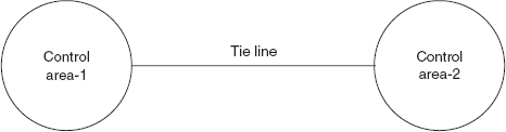
FIG. 8.1 Two control areas interconnected through a single tie line
Here, the control objective is to regulate the frequency of each area and to simultaneously regulate the power flow through the tie line according to an interarea power agreement.
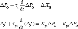
In the case of an isolated control area, the zero steady-state error in frequency (i.e., Δfsteady state = 0) can be obtained by using a proportional plus integral controller, whereas in two-control area case, proportional plus integral controller will be installed to give zero steady-state error in a tie-line power flow (i.e., ΔPTL = 0) in addition to zero steady-state error in frequency.
For the sake of convenience, each control area can be represented by an equivalent turbine, generator, and governor system.
In the case of a single control area, the incremental power (ΔPG−ΔPD) was considered by the rate of increase of stored KE and increase in area load caused by the increase in frequency.
In a two-area case, the tie-line power must be accounted for the incremental power balance equation of each area, since there is power f low in or out of the area through the tie line.
Power flow out of Control area-1 can be expressed as
where ∣E1∣ and ∣E2∣ are voltage magnitudes of Area-1 and Area-2, respectively, δ1 and δ2 are the power angles of equivalent machines of their respective areas, and XTL is the tie-line reactance.
If there is change in load demands of two areas, there will be incremental changes in power angles (Δδ1 and Δδ2). Then, the change in the tie-line power is
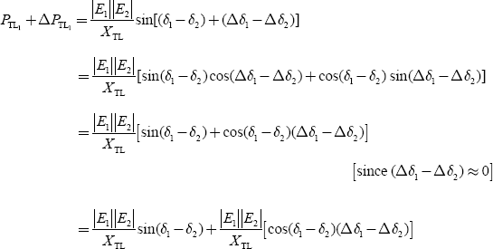
Therefore, change in incremental tie-line power can be expressed as

where
T12 is known as the synchronizing coefficient or the stiffness coefficient of the tie-line.
Equation (8.3) can be written as
where ![]() Static transmission capacity of the tie line.
Static transmission capacity of the tie line.
Consider the change in frequency as
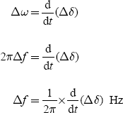
In other words,
Hence, the changes in power angles for Areas-1 and 2 are
and
Since the incremental power angles are related in terms of integrals of incremental frequencies, Equation (8.2) can be modified as
Δf1 and Δf2 are the incremental frequency changes of Areas-1 and 2, respectively. Similarly, the incremental tie-line power out of Area-2 is
where
Dividing Equation (8.6) by Equation (8.3), we get
Therefore, T21 = a12T12
and hence ∆PTL2 = a12∆PTL1 (8.7)
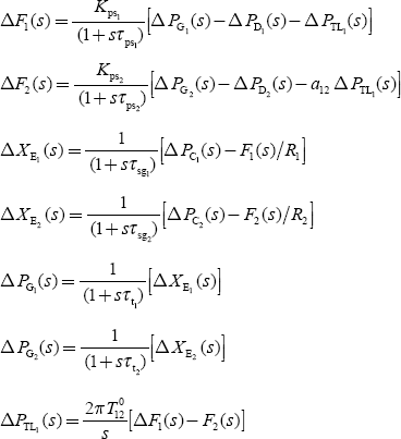
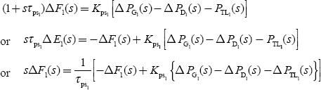
From Equation (7.25) (LFC-1), surplus power in p.u. is
For a two-area case, the surplus power can be expressed in p.u. as
Taking Laplace transform on both sides of Equation (8.8), we get
Rearranging the above equation as follows, we get

where

By comparing Equation (8.9) with single-area Equation (7.26), the only additional term is the appearance of signal ∆PTL1 (S)
Equation (8.9), can be represented in a block diagram model as shown in Fig. 8.2. Taking Laplace transformation on both sides of Equation (8.4), we get

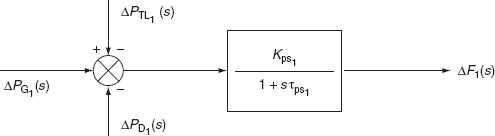
FIG. 8.2 Block diagram representation of Equation (8.9) (for Control area-1)

FIG. 8.3 Block diagram representation of Equations (8.10) and (8.11)
For Control area-2, we have
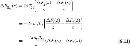
The block diagram representation of Equations (8.10) and (8.11) is shown in Fig. 8.3.
8.2 COMPOSITE BLOCK DIAGRAM OF A TWO-AREA CASE
By the combination of basic block diagrams of Control area-1 and Control area-2 and with the use of Figs. 8.2 and 8.3, the composite block diagram of a two-area system can be modeled as shown in Fig. 8.4.
8.3 RESPONSE OF A TWO-AREA SYSTEM—UNCONTROLLED CASE
For an uncontrolled case, ∆Pc1 = ∆Pc2 = 0, i.e., the speed-changer positions are fixed.
8.3.1 Static response
In this section, the changes or deviations, which result in the frequency and tie-line power under steady-state conditions following sudden step changes in the loads in the two areas, are determined.
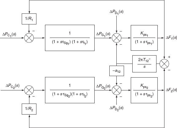
FIG. 8.4 Block diagram representation of a two-area system with an LFC
Let ∆PD1, ∆PD2 be sudden (incremental) step changes in the loads of Control area-1 and Control area-2, simultaneously.
∆PG1, ∆PG2 are the incremental changes in the generation in Area-1 and Area-2 as a result of the load changes.
Δf is the static change in frequency. This will be the same for both the areas and ∆PTL1 is the static change in the tie-line power transmitted from Area-1 to Area-2. Since only the static changes are being determined, the incremental changes in generation can be determined by the static loop gains. So, we have
and ![]() for static changes (8.13)
for static changes (8.13)
For the two areas, the dynamics are described by:
and
Under steady-state conditions, we have
After substituting Equations (8.12), (8.13), and (8.16) in Equations (8.14) and (8.15), we get
and
Since ∆PTL2 = −a12∆PTL1 and ∆f1 = ∆f2 = ∆f, from Equation (8.17), we have
Substituting ∆PTL1 from Equation (8.18(a)) in Equation (8.18), we get
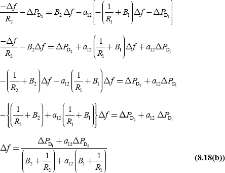
Substituting Δf from Equation (8.18(b)) in Equation (8.18 (a)), we get
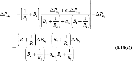
Equations (8.18(b)) and (8.18(c)) are modified as
Tie-line frequency,
Tie-line power,
where

Equations (8.19) and (8.20) give the values of the static changes in frequency and tie-line power, respectively, as a result of sudden step-load changes in the two areas. It can be observed that the frequency and tie-line power deviations do not reduce to zero in an uncontrolled case.
Consider two identical areas,
B1 = B2 = B, β1 = β2 = β, R1 = R2 = R and a12 = +1
Hence, from Equations (8.19) and (8.20), we have
and
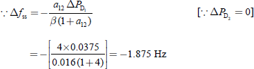
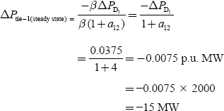
If a sudden load change occurs only in Area-2 (i.e.,∆PD1 = 0), then we have
and
Equations (8.23) and (8.24) illustrate the advantages of pool operation (i.e., grid operation) as follows:
- Equations (8.19) represents the change in frequency according to the change in load in either of a two-area system interconnected by a tie line. When considering that those two areas are identical, Equation (8.19) becomes Equation (8.21). Hence, it is concluded that if a load disturbance occurs in only one of the areas (i.e., ∆PD1 = 0 or ∆PD2 = 0), the change in frequency (Δ f) is only half of the steady-state error, which would have occurred with no interconnection (i.e., an isolated case). Thus, with several systems interconnected, the steady-state frequency error would be reduced.
- Half of the added load (in Area-2) is supplied by Area-1 through the tie line.
The above two advantages represent the necessity of interconnecting the systems.
8.3.2 Dynamic response
To describe the dynamic response of the two-area system as shown in Fig. 8.4, a system of seventh-order differential equations is required. The solution of these equations would be tedious. However, some important characteristics can be brought out by an analysis rendered simple by the following assumptions. A power system of two identical control areas is considered for the analysis:
- τgt = τt = 0 for both the areas.
- The damping constants of two areas are neglected,
i.e., B1 = B2 = 0
By virtue of the second assumption, Equations (8.14) and (8.15) become
Taking Laplace transformation on both sides of Equations (8.25) and (8.26) and by rearrangement, we get
From the block diagram of Fig. 8.4, the following equations can be obtained:

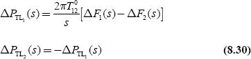
(![]() , since two control areas are identical)
, since two control areas are identical)
By solving Equations (8.27)–(8.30), we get
From the above equation, the following observations can be made:
(i) The denominator is of the form:
where
and α and ω2 are both real and positive. Hence, it can be concluded from the roots of characteristic equation that the time response is stable and damped.
The three conditions are:
If α = ωn, system is critically damped
α > ωn, system becomes overdamped

where α = damping factor or decrement of attenuation
ω0 = damped angular frequency ![]()
Since parameter α also depends on B, but ![]() in practice, therefore, the effect of coefficient B is neglected on damping.
in practice, therefore, the effect of coefficient B is neglected on damping.
(ii) After a disturbance, the change in tie-line power oscillates at the damped angular frequency.
(iii) The damping of the tie-line power variation is strongly dependent upon the parameter α, which is equal to ![]() . Since f 0 and H are essentially constant, the damping is a function of the R parameters. If the R value is low, damping becomes strong and vice versa.
. Since f 0 and H are essentially constant, the damping is a function of the R parameters. If the R value is low, damping becomes strong and vice versa.
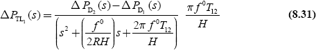
The transient change in the tie-line power will be of undamped oscillations of frequency, ωo = ω.
If R = ∞, i.e., if the speed governor is not present (α = 0), the variation in frequency deviation and the tie-line power would be as shown in Fig. 8.5.
It can be seen that the steady-state frequency deviation is the same for both the areas and does not vanish. The tie-line power deviation also does not become zero.
Although the above approximate analysis has confirmed stability, it has been found through more accurate analyses that with certain parameter combinations, the system becomes unstable.
FIG. 8.5 Frequency deviation and tie-line power change following a step-load change in Area-2 (two areas are identical)
Example 8.1: A two-identical area power system has the following parameters (Fig. 8.6(a)):
Power system gain constant, Kps = 105
Power system time constant, τps = 22 s
Speed regulation, R = 2.5
Normal frequency, f 0 = 50 Hz
Governor time constant, τsg = 0.3 s
Turbine time constant, τt = 0.5 s
Integration time constant, ki = 0.15
Bias parameter, b = 0.326
2πT12 = 0.08
Plot the change in the tie-line power and change in frequency of control-area 1 if there exists a step-load change of 2% in Area-1 (Fig. 8.6(b)).


FIG. 8.6 (a) Simulation block diagram for a two-identical area system of Example 8.1; (b) frequency and tie-line response for Example 8.1
Example 8.2: A two-area power system has the following parameters (Fig. 8.7(a)):
For Area-1:
Power system gain constant, Kps = 120
Power system time constant, Ƭps = 20 s
Speed regulation, R = 2.5
Normal frequency, f 0 = 50 Hz
Governor time constant, Ƭsg = 0.2 s
Turbine time constant, Ƭt = 0.4 s
Integration time constant, ki = 0.1
Bias parameter, b = 0.425
For Area-2:
Power system gain constant, Kps = 100
Power system time constant, Ƭps = 22 s
Speed regulation, R = 3
Normal frequency, f 0= 50 Hz
Governor time constant, Ƭsg = 0.3 s
Turbine time constant, Ƭt = 0.5 s
Integration time constant, ki = 0.15
Bias parameter, b = 0.326
2πT12 = 0.08
Plot the change in the tie-line power and change in frequency of Control-area 1 if there exists a step-load change of 2% in Area-1 (Fig. 8.7(b)).
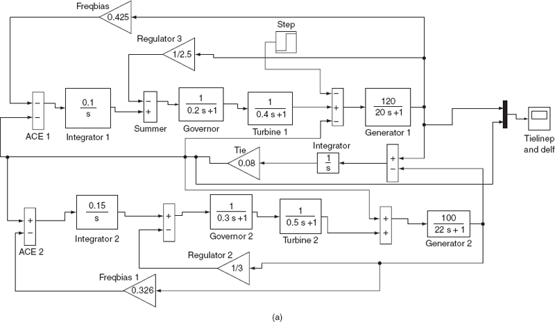
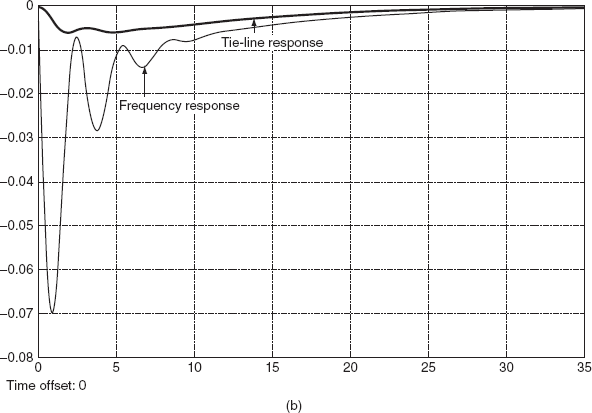
FIG. 8.7 (a) Simulation block diagram of Example 8.2; (b) Frequency and tie-line power response of Example 8.2
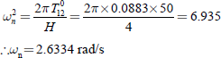
Example 8.3: Determine the frequency of oscillations of the tie-line power deviation for a two-identical-area system given the following data:
R = 3.0 Hz / p.u.; H = 5 s; f 0 = 60 Hz
The tie-line has a capacity of 0.1 p.u. and is operating at a power angle of 45°.
Solution:
The synchronizing-power coefficient of the line is given by
T012 = Pm cos δ12 = 0.1 × cos 45° = 0.0707 p.u.
Hence, the frequency of oscillations is given by

8.4 AREA CONTROL ERROR —TWO-AREA CASE
In a single-area case, ACE is the change in frequency. The steady-state error in frequency will become zero (i.e., Δfss = 0) when ACE is used in the integral-control loop.
In a two-area case, ACE is the linear combination of the change in frequency and change in tie-line power. In this case to make the steady-state tie-line power zero (i.e., ΔPTL = 0), another integral-control loop for each area must be introduced in addition to the integral frequency loop to integrate the incremental tie-line power signal and feed it back to the speed-changer.
Thus, for Control area-1, we have
where b1 = constant = area frequency bias. Taking Laplace transform on both sides of Equation (8.33), we get
Similarly, for Control area-2, we have
8.5 COMPOSITE BLOCK DIAGRAM OF A TWO-AREA SYSTEM (CONTROLLED CASE)
By the combination of basic block diagrams of Control area-1 and Control area-2 and with the use of Figs. 8.2 and 8.3, the composite block diagram of a two-area system can be modeled as shown in Fig. 8.4. Figure 8.8 can be obtained by the addition of integrals of ACE1 and ACE2 to the block diagram shown in Fig. 8.4. It represents the composite block diagram of a two-area system with integral-control loops. Here, the control signals ∆Pc1(s) and ∆Pc2(s) are generated by the integrals of ACE1 and ACE2. These control errors are obtained through the signals representing the changes in the tie-line power and local frequency bias.
8.5.1 Tie-line bias control
The speed-changer command signals will be obtained from the block diagram shown in Fig. 8.6 as
and
The constants KI1 and KI2 are the gains of the integrators. The first terms on the right-hand side of Equations (8.36) and (8.37) constitute and are known as tie-line bias controls. It is observed that for decreases in both frequency and tie-line power, the speed-changer position decreases and hence the power generation should decrease, i.e., if the ACE is negative, then the area should increase its generation.
So, the right-hand side terms of Equations (8.36) and (8.37) are assigned a negative sign.
8.5.2 Steady-state response
That the control strategy, described in the previous section, eliminates the steady-state frequency and tie-line power deviations that follow a step-load change, can be proved as follows:

FIG. 8.8 Two-area system with integral control
Let the step changes in loads ∆PD1 and ∆PD2 simultaneously occur in Control area-1 and Control area-2, respectively, or in either area. A new static equilibrium state, i.e., steady-state condition is reached such that the output signal of all integrating blocks will become constant. In this case, the speed-changer command signals ∆Pc1 and ∆Pc2 have reached constant values. This obviously requires that both the integrands (input signals) in Equations (8.36) and (8.37) be zero.
Input of integrating block ![]() is
is
Input of integrating block ![]() is
is
and input of integrating block ![]() is
is
Equations (8.38) and (8.39) are simultaneously satisfied only for ∆PTL1(ss) = ∆PTL2(ss) = 0 and ∆f1(ss) = ∆f2(ss) = 0.
Thus, under a steady-state condition, change in tie-line power and change in frequency of each area will become zero. To achieve this, ACEs in the feedback loops of each area are integrated.
The requirements for integral control action are:
- ACE must be equal to zero at least one time in all 10-minute periods.
- Average deviation of ACE from zero must be within specified limits based on a percentage of system generation for all 10-minute periods.
The performance criteria also apply to disturbance conditions, and it is required that:
- ACE must return to zero within 10-minute periods.
- Corrective control action must be forthcoming within 1 minute of a disturbance.
8.5.3 Dynamic response
The determination of the dynamic response of the two-area model shown in Fig. 8.6 is more difficult. This is due to the fact that the system of equations to be solved is of the order of nine. Therefore, actual solution is not attempted. But the results obtained from an approximate analysis of a two-identical-area power system for three different values of the parameter ‘b’, are presented in Figs. 8.9(a), (b), and (c).
The graphs of Fig. 8.9(a) correspond to the case of b = 0. It can be seen that the tie-line power deviation reduces to zero while the frequency does not.
The graphs of Fig. 8.9(b) correspond to the other extreme case of b = ∞. Now, the frequency error vanishes. But, the tie-line power does not vanish.
The graphs of Fig. 8.9(c) show an intermediate case wherein both the frequency and the tie-line power errors decrease to zero. This is the desired case.
Therefore, it can be concluded that the stability is not always guaranteed. Hence, there is a need for proper parameter selection and adjustment of their values.
8.6 OPTIMUM PARAMETER ADJUSTMENT
The graphs given in Fig. 8.9(c) stress the need for proper parameter settings. The choice of b and KI constants affects the transient response to load changes. The frequency bias b should be high enough such that each area adequately contributes to frequency control. It is proved that choosing b = β gives satisfactory performance of the interconnected system.
The integrator gain KI should not be too high, otherwise, instability may result. Also the time interval at which LFC signals are dispatched, two or more seconds, should be low enough so that LFC does not attempt to follow random or spurious load changes.
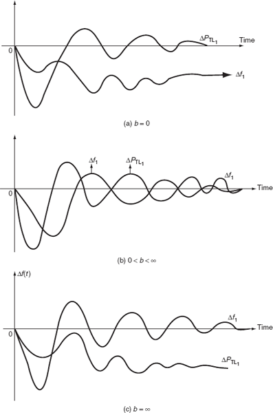
FIG. 8.9 Approximate dynamic response of two-identical-area power systems with three different values of b parameters
First, a set of parameters, which ensure stability of the control, is selected. For example, b1 and b2 cannot both be zero, i.e., one of them should be chosen for the control strategy. Later, the values of these parameters are adjusted so that a best or an optimum response is obtained. In other words, the values of parameters, which give rise to an optimum response, are to be determined.
The procedure is as follows:
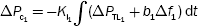
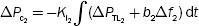
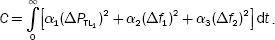
The popular error criterion, known as the integral of the squared errors (ISE), is chosen for the control parameters ∆f1, ∆f2, and ∆PTL1. For a two-area system, the ISE criterion function C would be
where α1, α2, and α3 are the weight factors, which provide appropriate importance, i.e., weightage to the errors ∆PTL1, Δf1, and Δf2. There is no need to choose ∆PTL2, since ∆PTL2 = a12∆PTL1.
Since Δf1 and Δf2 behave in a similar manner, we need to consider only one of them. So, let us consider Δf1 only. This is a parameter selection. Then, α3 = 0. Also, let α2 = α. Since, we are interested only in the relative magnitudes of C for parameter setting, we can set α1 = 1.
With these, Equation (7.41) reduces to
For a two-area system, ∆PTL2 and Δf1 would be functions of the integrator gain constants KI1 and KI2 as well as the frequency bias parameters b1 and b2.
The procedure for obtaining the optimum parameter values would be as follows:
First, a convenient and suitable value is chosen for the weight factor ‘α’. Then, for different assumed values of KI1, KI2, b1, and b2, the values of ∆PTL1 and Δf1 are determined at different instants of time. With these values and α, the value of C is computed using Equation (8.42). The set of values of KI1, KI2, b1, and b2 for which C is a minimum is the optimum one.
If we consider the two identical areas, then the number of parameters reduces to two, viz., KI1 = KI2 = K1 and b1 = b2 = b. In this case, values of C for different values of KI and b can be plotted as shown in Fig. 8.10. As can be seen, the variation of C with KI for different fixed values of b is plotted to get a family of curves called constant-b contours. For illustration, only three curves are shown in Fig. 8.10. In practice, a number of curves have to be determined and drawn. It can be seen that C is minimum for b = 0.2 and KI = 1.0.
In this case, the optimum control strategy would, therefore, be
and
In practice, the frequency and tie-line power deviations are measured at fixed intervals of time in a sample-data fashion. The sampling rate (the rate at which the frequency deviation and tie-line power deviation samples are measured) should be sufficiently high to avoid errors due to sampling.
Note: LFC provides enough control during normal changes in load and frequency, i.e., changes that are not too large. During emergencies, when large imbalances between generation and load occur, LFC is bypassed and other emergency controls are applied, which is beyond the scope of this book.
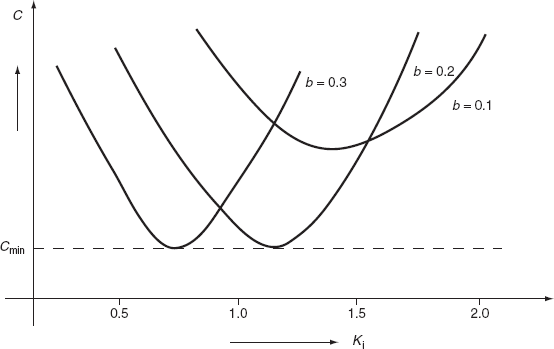
FIG. 8.10 Constant b-contours of the ISE criterion function C
8.7 LOAD FREQUENCY AND ECONOMIC DISPATCH CONTROLS
Economic load dispatch and LFC play a vital role in modern power system. In LFC, zero steady-state frequency error and a fast, dynamic response were achieved by integral controller action. But this control is independent of economic dispatch, i.e., there is no control over the economic loadings of various generating units of the control area.
Some control over loading of individual units can be exercised by adjusting the gain factors (KI) of the integral signal of the ACE as fed to the individual units. But this is not a satisfactory solution.
A suitable and satisfactory solution is obtained by using independent controls of load frequency and economic dispatch. The load frequency controller provides a fast-acting control and regulates the system around an operating point, whereas the economic dispatch controller provides a slow-acting control, which adjusts the speed-changer settings every minute in accordance with a command signal generated by the central economic dispatch computer.
EDC—economic dispatch controller
CEDC—central economic dispatch computer
The speed-changer setting is changed in accordance with the economic dispatch error signal, (i.e., PG (desired) − PG (actual)) conveniently modified by the signal ∫ ACE dt at that instant of time. The central economic dispatch computer (CEDC) provides the signal PG (desired), and this signal is transmitted to the local economic dispatch controller (EDC). The system they operate with economic dispatch error is only for very short periods of time before it is readily used (Fig. 8.11).
This tertiary control can be implemented by using EDC and EDC works on the cost characteristics of various generating units in the area. The speed-changer settings are once again operated in accordance with an economic dispatch computer program.

FIG. 8.11 Load frequency and economic dispatch control of the control area of a power system
The CEDCs are provided at a central control center. The variable part of the load is carried by units that are controlled from the central control center. Medium-sized fossil fuel units and hydro-units are used for control. During peak load hours, lesser efficient units, such as gas-turbine units or diesel units, are employed in addition; generators operating at partial output (with spinning reserve) and standby generators provide a reserve margin.
The central control center monitors information including area frequency, outputs of generating units, and tie-line power flows to interconnected areas. This information is used by ALFC in order to maintain area frequency at its scheduled value and net tie-line power flow out of the area at its shedding value. Raise and lower reference power signals are dispatched to the turbine governors of controlled units.
Economic dispatch is co-ordinated with LFC such that the reference power signals dispatched to controlled units move the units toward their economic loading and satisfy LFC objectives.
8.8 DESIGN OF AUTOMATIC GENERATION CONTROL USING THE KALMAN METHOD
A modern gigawatt generator with its multistage reheat turbine, including its automatic load frequency control (ALFC) and automatic voltage regulator (AVR) controllers, is characterized by an impressive complexity. When all its non-negligibility dynamics are taken into account, including cross-coupling between control channels, the overall dynamic model may be of the twentieth order.
The dimensionality barrier can be overcome by means of computer-aided optimal control design methods originated by Kalman. A computer-oriented technique called optimum linear regulator (OLR) design has proven to be particularly useful in this regard.
The OLR design results in a controller that minimizes both transient variable excursions and control efforts. In terms of power system, this means optimally damped oscillation with minimum wear and tear of control valves.
OLR can be designed using the following steps:
- Casting the system dynamic model in state-variable form and introducing appropriate control forces.
- Choosing an integral-squared-error control index, the minimization of which is the control goal.
- Finding the structure of the optimal controller that will minimize the chosen control index.
8.9 DYNAMIC-STATE-VARIABLE MODEL
The LFC methods discussed so far are not entirely satisfactory. In order to have more satisfactory control methods, optimal control theory has to be used. For this purpose, the power system model must be in a state-variable model.
8.9.1 Model of single-area dynamic system in a state-variable form
From the block diagram of an uncontrolled single-area system shown in Fig. 8.12, we get the following ‘s-domain’ equations:

In time domain, the above equations can be expressed as

FIG. 8.12 State-space model of a single-area system
Let us choose the state variables  , input, u = ΔPC, and disturbance, d = ΔPD
The above equations are written in a state-variable form:
The state equation would then be written in a more general form as
where x is the n-dimensional state vector, u the m-dimensional control-force vector = [u] = [ΔPc], and p the disturbance force vector = [p] = [ΔPD].
8.9.2 Optimum control index (I)
The optimum linear regulator design is based on the integral-squared-error index of the form.
where q’s and r’s are positive penalty factors. Let us consider index I for a single-area system as
Here, the idea of optimum control is to minimize the index (I). Consider the term q3 (Δ f)2, squaring of frequency error will contribute to ‘I’ independent of its sign. If Δf is doubled, its contribution to ‘I’ will quadruple. The integral causes Δf to add to ‘I’ during its entire duration. The penalty factors qi distribute the penalty weight among the state-variable errors. If the error in a particular variable is of little significance, we simply set its penalty factor to zero.
Similarly, in the case of control-force increments, the penalty factors ri distribute the penalties among the m control force. (Here, none of r’s are set to zero.) If they are set to zero, then the control force will assume an infinite magnitude without affecting ‘I’. An infinite control force could do its correcting job in zero time. This would obviously be a very unrealistic regulator.
If all q’s and r’s constitute the diagonal elements of the two penalty matrices, then we have

Index-I in a compact form is
8.9.3 Optimum control problem and strategy
The task that an OLR or an optimum controller must perform is the fulfillment of the optimum control problem, which can be stated as follows: consider a system that is initially under steady-state condition. If it is disturbed by a set of step type of disturbances, it goes through a transient state first. It is required that, after the expiry of the transient period, it should return to the original or new prescribed steady-state condition. The problem is to determine the set of control forces ![]() which will not only take the system to the original or new prescribed steady state, but will also do so by simultaneously minimizing the chosen control criterion function or optimum control index (I).
which will not only take the system to the original or new prescribed steady state, but will also do so by simultaneously minimizing the chosen control criterion function or optimum control index (I).
The value of ![]() which fulfills the above optimum control requirement, is the desired optimum control strategy. An optimum controller or OLR is the one that carries out the above strategy.
which fulfills the above optimum control requirement, is the desired optimum control strategy. An optimum controller or OLR is the one that carries out the above strategy.
8.9.4 Dynamic equations of a two-area system
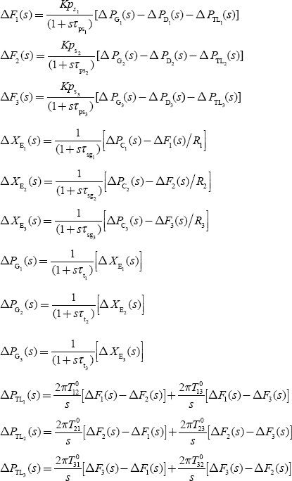
From the block diagram of uncontrolled two-area systems shown in Fig. 8.4, get the following ‘s-domain’ equations:
where XE1(s) and XE2(s) are the Laplace transforms of the movements of the main positions in the speed-governing mechanisms of the two areas.
By taking inverse Laplace transform for the above equations, we get a set of seven differential equations. These are the time-domain equations, which describe the small-disturbance dynamic behavior of the power system.
Consider the first equation,
Taking the inverse Laplace transform of the above equation, we get
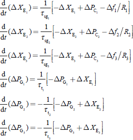
In a similar way, the remaining equations can be rearranged and an inverse Laplace transform is found. Then, the entire set of differential equations is

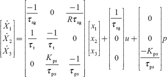
8.9.4.1 State variables and state-variable model
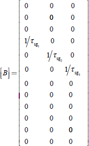
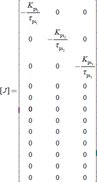
The state variables are a minimum number of those variables, which contain sufficient information about the past history with which all future states of the system can be determined for known control inputs. For the two-area system under consideration, the state variables would be Δf1, Δf2, ∆XE1, ∆XE2, ∆Psg1, ∆Psg2 and ∆PTL1; seven in number. Denoting the above variables by x1, x2, x3, x4, x5, x6, and x7 and arranging them in a column vector as
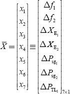
where ![]() is called a state vector.
is called a state vector.
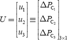
The control variables ∆Pc1 and ∆Pc2 are denoted by the symbols u1 and u2, respectively, as
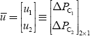
where ū is called the control vector or the control-force vector.
The disturbance variables ∆PD1 and ∆PD2, since they create perturbations in the system, are denoted by p1 and p2, respectively, as
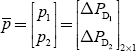
where ![]() is called the disturbance vector.
is called the disturbance vector.
The above state equations can be written in a matrix form as

where ![]() ; i = 1, 2, 3, … 7.
; i = 1, 2, 3, … 7.
The above matrix equation can be written in the vector form as
where [A] is called the system matrix, [B] the input distribution matrix, and [J] the disturbance distribution matrix.
In the present case, their dimensions are (7 × 7), (7 × 2), and (7 × 2), respectively. Equation (8.45) is a shorthand form of Equation (8.44), and Equation (8.44) constitutes the dynamic ‘state-variable model’ of the considered two-area system.
The differential equations can be put in the above form only if they are linear. If the differential equations are non-linear, then they can be expressed in the more general form as
8.9.5 State-variable model for a three-area power system
The block diagram representation of this model is shown in Fig. 8.13.

FIG. 8.13 Three-area model
From the block diagram, the following equations are written as
Taking the inverse Laplace transform for the above equations, which we get in a similar way, the remaining equations can be rearranged and the inverse Laplace transform can be found. Then, the entire set of differential equations is

and ![]()
and ![]()
and ![]()
The above equations are written in a vector form as shown below:
where ![]()

where X is called a state vector.
The control variables ∆Pc1, ∆Pc2, and ∆Pc1 are denoted by the symbols u1, u2, and u3, respectively, as
where u is called the control vector or the control-force vector.
The disturbance variables ∆PD1, ∆PD2, and ∆PD1, since they create perturbations in the system, are denoted by p1, p2, and p3, respectively, as
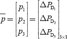
where ![]() is called the disturbance vector.
is called the disturbance vector.
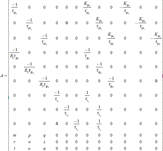
where |
m |
= |
2π(T012 + T013) |
|
n |
= |
2π(T021 + T023) |
|
o |
= |
2π(T031 + T032) |
|
p |
= |
−2πT012 |
|
q |
= |
−2πT013 |
|
r |
= |
−2πT021 |
|
s |
= |
−2πT023 |
|
t |
= |
−2πT031 |
|
ū |
= |
−2πT032 |
8.9.6 Advantages of state-variable model
The state-variable modeling of a power system offers the following advantages:
- Modern control theory is based upon this standard form.
- By arranging system parameters into matrices [A], [B], and [J], a very organized methodology of solving system equations, either analytically or by computer, is developed. This is important for large systems where a lack of organization easily results in errors.
Example 8.4: Two interconnected Area-1 and Area-2 have the capacity of 2,000 and 500 MW, respectively. The incremental regulation and damping torque coefficient for each area on its own base are 0.2 p.u. and 0.8 p.u., respectively. Find the steady-state change in system frequency from a nominal frequency of 50 Hz and the change in steady-state tie-line power following a 750 MW change in the load of Area-1.
Solution:
Rated capacity of Area-1 = P1(rated) = 2,000 MW
Rated capacity of Area-2 = P2(rated) = 500 MW
Speed regulation, R = 0.2 p.u.
Nominal frequency, f = 50 Hz
Change in load power of Area-1, ΔP1 = 75 MW
Speed regulation, R = 0.2 = 0.2 p.u. × 50 = 10 Hz/p.u. MW
Damping torque coefficient, B = 0.8 p.u. MW/p.u. Hz
Change in load of Area-1, ∆PD1 = 75 MW
p.u. change in load of Area-1 ![]()
p.u. change in load of Area-2 ![]()
Steady-state change in system frequency, ![]()

where ![]()
Steady-state change in tie-line power following load change in Area-1:


Example 8.5: Solve Example 8.4, without governor control action.
Solution:
Without the governor control action, R = 0

Steady-state change in tie-line power following load change in Area-1:
It is observed from the result that the power flow through the tie line is the same in both the cases of with governor action and without governor action, since it does not depend on speed regulation R.
Example 8.6: Find the nature of dynamic response if the two areas of the above problem are of uncontrolled type, following a disturbance in either area in the form of a step change in electric load. The inertia constant of the system is given as H = 3 s and assume that the tie line has a capacity of 0.09 p.u. and is operating at a power angle of 30o before the step change in load.
Solution:
Given:
Speed regulation, R = 0.2 p.u. = 0.2 × 50 = 10 Hz/p.u. MW
Damping coefficient, B = 0.8 p.u. MW/p.u. Hz
Inertia constant, H = 3 s
Nominal frequency, f 0 = 50 Hz
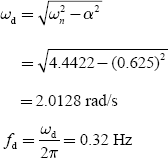
Tie-line capacity, ![]()
From the theory of dynamic response, we know that

It is observed that the damped oscillation type of dynamic response has resulted since α < ωn:
∴ Damped angular frequency
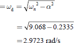
∴ Damped frequency = fd ![]()
Example 8.7: Two control areas have the following characteristics:
Area-1: |
Speed regulation = 0.02 p.u. |
|
Damping coefficient = 0.8 p.u. |
|
Rated MVA = 1,500 |
Area-2: |
Speed regulation = 0.025 p.u. |
|
Damping coefficient = 0.9 p.u. |
|
Rated MVA = 500 |
Determine the steady-state frequency change and the changed frequency following a load change of 120 MW, which occurs in Area-1. Also find the tie-line power flow change.
Solution:
Given R1 = 0.1 p.u.; R2 = 0.098 p.u.
B1 = 0.8 p.u.; B2 = 0.9 p.u.
P1 rated = 1,500 MVA; P2 rated = 1,500 MVA
Change in load of Area-1,
∆PD1 = 120 MW, ∆PD2 = 0
p.u. change in load of Area-1 ![]()
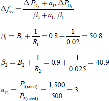
∴ Steady-state frequency change,

i.e., Steady-state change in frequency, ∆fss |
= |
0.0012415 × 50 |
|
= |
0.062 Hz |
∴ New value of frequency, f = f0 − ∆fss |
= |
50 − 0.062 |
|
= |
49.937 Hz |
Steady-state change in tie-line power
Example 8.8: In Example 8.6, if the disturbance also occurs in Area-2, which results in a change in load by 75 MW, determine the frequency and tie-line power changes.
Solution:
Change in load of Area-1, ∆PD1 = 120 MW
p.u. change in load of Area-1 ![]()
Change in load of Area-2, ∆PD2 = 75 MW
p.u. change in load of Area-2 ![]()
Steady-state frequency change,
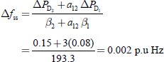
∴ Steady-state frequency change = 0.002 × 50 = 0.1 Hz
∴ New value of frequency = f 0 − Δfss = 50 − 0.1 = 49.899 Hz
Steady-state change in tie-line power,

Example 8.9: Two areas of a power system network are interconnected by a tie line, whose capacity is 250 MW, operating at a power angle of 45o. If each area has a capacity of 2,000 MW and the equal speed-regulation coefficiency of 3 Hz/p.u. MW, determine the frequency of oscillation of the power for a step change in load. Assume that both areas have the same inertia constants of H = 4 s. If a step-load change of 100 MW occurs in one of the areas, determine the change in tie-line power.
Solution:
Given:
Tie-line capacity, Ptie(max) = 250 MW
Power angle of two areas, (δ01 − δ02) = 457°
Capacity of each area, Prated = 2,000 MW
Speed-regulation coefficient = R1 = R2 = R = 3Hz/p.u. MW
Inertia constant, H = 4 s


Since, α < ωn, the dynamic response will be of a damped oscillation type.
Damped angular frequency,

∴ Frequency of oscillation, ![]()
If a step-load change of 100 MW occurs in any one of the areas, the total load change will be shared equally by both areas since the two areas are equal, i.e., a power of ![]() will flow from the other area into the area where a load change occurs.
will flow from the other area into the area where a load change occurs.
Example 8.10: Two power stations A and B of capacities 75 and 200 MW, respectively, are operating in parallel and are interconnected by a short transmission line. The generators of stations A and B have speed regulations of 4% and 2%, respectively. Calculate the output of each station and the load on the interconnection if
- the load on each station is 100 MW,
- the loads on respective bus bars are 50 and 150 MW, and
- the load is 130 MW at Station A bus bar only.
Solution:
Given:
Capacity of Station-A = 75 MW
Capacity of Station-B = 200 MW
Speed regulation of Station-A generator, RA = 4%
Speed regulation of Station-B generator, RB = 2%
(a) If the load on each station = 100 MW
Speed regulation ![]()

From Equations (8.48) and (8.49), we have
0.000533P1 = 0.0001P2
5.33P1 = P2 (8.50)
P1 + P2 = 200
Substituting Equation (8.50) in Equation (8.47), we get
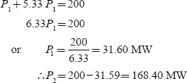
The power generations and tie-line power are indicated in Fig. 8.14(a).
(b) If the load on respective bus bars are 50 and 150 MW, then we have
i.e., P1 + P2 = 50 + 150 = 200 MW
5.33 P1 = P2
P1 + 5.33 P1 = 200
⇒ 6.33P1 = 200
P1 = 31.6 MW
∴ P2 = 200 − 31.60 = 168.4 MW
The power generations and tie-line power are indicated in Fig. 8.14(b).

FIG. 8.14 (a) Illustration for Example 8.10; (b) illustration for Example 8.10; (c) illustration for Example 8.10
(c) If the load is 130 MW at A only, then we have
P1 + P2 = 130
5.33P1 = P2
∴ P1 = 5.33 P1 = 130
6.33P1 = 130
⇒ P1 = 20.537 MW
∴ P2 = 130 − P1 = 109.462 MW
The power generations and tie-line power are indicated in Fig. 8.14(c).
Example 8.11: The two control areas of capacity 2,000 and 8,000 MW are interconnected through a tie line. The parameters of each area based on its own capacity base are R = 1 Hz/p.u. MW and B = 0.02 p.u. MW/Hz. If the control area-2 experiences an increment in load of 180 MW, determine the static frequency drop and the tie-line power.
Solution:
Capacity of Area-1 = 2,000 MW
Capacity of Area-2 = 8,000 MW
Taking 8,000 MW as base,
∴ Speed regulation of Area-1, ![]()
Damping coeffi cient of Area-1, ![]()
Speed regulation of Area-2, R2 = 1 Hz / p.u. MW
Damping coefficient of Area-2, B2 = 0.02 p.u. MW/ Hz
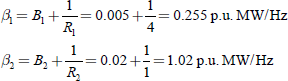
Given an increment of Area-2 in load, ![]()
∴ Static change in frequency,
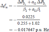
Static change in tie-line power,
Note: Here, a12 value determination is not required since values of R1, B1, and β1 are obtained according to the base values.
Alternate method:
Find ![]() Then, obtain the ∆f(ss) and ∆Ptie(ss) values.
Then, obtain the ∆f(ss) and ∆Ptie(ss) values.
Here, there is no need to obtain, R1, B1, R2, and B2 separately.
Example 8.12: Two generating stations A and B having capacities 500 and 800 MW, respectively, are interconnected by a short line. The percentage speed regulations from no-load to full load of the two stations are 2 and 3, respectively. Find the power generation at each station and power transfer through the line if the load on the bus of each station is 200 MW.
Solution:
Given data:
Capacity of Station-A = 500 MW
Capacity of Station-B = 800 MW
Percentage speed regulation of Station-A = 2% = 0.02
Percentage speed regulation of Station-B = 3% = 0.03
Load on bus of each station = PDA = PDB = 200 MW
Total load, PD = 400 MW
Speed regulation of Station-A:
Speed regulation of Station-B:
Let PGA be the power generation of Station-A and PGB the power generation of Station-B:
PGB = Total load − PGA = (400 − PGA)
⇒ 0.002PGA = 0.001875 (400 − PGA)
= 0.75 = 193.55 MW
(0.002 + 0.001875) PGA = 0.75
⇒ |
PGA |
= |
193.55 MW |
|
PGB |
= |
206.45 MW |
|
PGA |
= |
193.55 MW |
∴ |
PGB |
= |
206.45 MW |
The power transfer through the line from Station-B to station-A
= PGB − (load at bus bar of B)
= 206.45 − 200
= 6.45 MW
Example 8.13: Two control areas of 1,000 and 2,000 MW capacities are interconnected by a tie line. The speed regulations of the two areas, respectively, are 4 Hz/p.u. MW and 2.5 Hz/p.u. MW. Consider a 2% change in load occurs for 2% change in frequency in each area. Find steady-state change in frequency and tie-line power of 10 MW change in load occurs in both areas.
Solution:
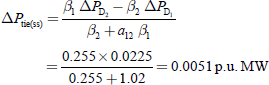
Capacity of Area-1 = 1,000 MW
Capacity of Area-2 = 2,000 MW
Speed regulation of Area-1, R1 = 4 Hz/p.u. MW (on 1,000-MW base)
Speed regulation of Area-2, R2 = 2 Hz/p.u. MW
Let us choose 2,000 MW as base, 2% change in load for 2% change in frequency
Damping coeffi cient of Area-1,
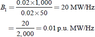
Similarly, damping coefficient of Area-2 on 2,000-MW base
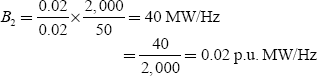
Speed regulation of Area - 1on 2,000-MW base = R1
Speed regulation of Area-2, R2 = 2 Hz/p.u. MW

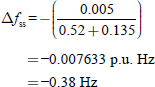
If a 10-MW change in load occurs in Area-1, then we have
Steady-state change in frequency,
Steady-state change in frequency,
or Δf(ss) = −0.007633 × 50 = 0.38 Hz
Steady-state change in tie-line power:
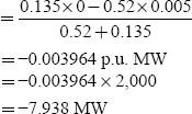
i.e., the power transfer of 7.938 MW is from Area-2 to Area-1.
If a 10-MW change in load occurs in Area-2, then we have
∴ Steady-state change in frequency,
Steady-state change in tie-line power:
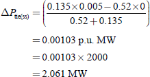
i.e., A power of 2.061 MW is transferred from Area-1 to Area-2.
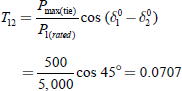
Example 8.14: Two similar areas of equal capacity of 5,000 MW, speed regulation R = 3 Hz/p.u. MW, and H = 5 s are connected by a tie line with a capacity of 500 MW, and are operating at a power angle of 45o. For the above system, the frequency is 50 Hz; find:
- The frequency of oscillation of the system.
- The steady-state change in the tie-line power if a step change of 100 MW load occurs in Area-2.
- The frequency of oscillation of the system in the speed-governor loop is open.
Solution:
Given:
Capacity of each control area = P1(rated) P2(rated) = 500 MW
Speed regulation, R = 2 Hz/p.u. MW
Inertia constant, H = 5 s
Power angle = 45o
Supply frequency, f 0 = 50 Hz
(a) Stiffness coefficient,
Since α < ωn, damped oscillations will be present.
∴ Damped angular frequency,
(b) Since the two areas are similar, each area will supply half of the increased load:
ΔPtie = 50 MW from Area-1 to Area-2.
If the speed-governor loop is open, then ![]()
Damped angular frequency,

KEY NOTES
- An extended power system can be divided into a number of LFC areas, which are interconnected by tie lines. Such an operation is called a pool operation.
The basic principle of a pool operation in the normal steady state provides:
- Maintaining of scheduled interchanges of tie-line power.
- Absorption of own load change by each area.
- The advantages of a pool operation are as follows:
- Half of the added load (in Area-2) is supplied by Area-1 through the tie line.
- The frequency drop would be only half of that which would occur if the areas were operating without interconnection.
- The speed-changer command signals will be:
and
The constants K12 and K12 are the gains of the integrators. The first terms on the right-hand side of the above equations constitute what is known as a tie-line bias control.
- The load frequency controller provides a fast-acting control and regulates the system around an operating point, whereas the EDC provides a slow-acting control, which adjusts the speed-changer settings every minute in accordance with a command signal generated by the CEDC.
SHORT QUESTIONS AND ANSWERS
- What are the advantages of a pool operation?
The advantages of a pool operation (i.e., grid operation) are:
- Half of the added load (in Area-2) is supplied by Area-1 through the tie line.
- The frequency drop would be only half of that which would occur if the areas were operating without interconnection.
- Without speed-changer position control, can the static frequency deviation be zero?
No, the static frequency deviation cannot be zero.
- State the additional requirement of the control strategy as compared to the single-area control.
The tie-line power deviation due to a step-load change should decrease to zero.
- Write down the expressions for the ACEs.
The ACE of Areas-1 and 2 are:
ACE1 (S) = ∆PTL1 (S) + b1∆F1(S).
ACE2 (S) = ∆PTL2 (S) + b2∆F2(S).
- What is the criterion used for obtaining optimum values for the control parameters?
Integral of the sum of the squared error criterion is the required criterion.
- Give the error criterion function for the two-area system.
- What is the order of differential equation to describe the dynamic response of a two-area system in an uncontrolled case?
It is required for a system of seventh-order differential equations to describe the dynamic response of a two-area system. The solution of these equations would be tedious.
- What is the difference of ACE in single-area and two-area power systems?
In a single-area case, ACE is the change in frequency. The steady-state error in frequency will become zero (i.e., Δfss = 0) when ACE is used in an integral-control loop.
In a two-area case, ACE is the linear combination of the change in frequency and change in tie-line power. In this case to make the steady-state tie-line power zero (i.e., ΔPTL = 0), another integral-control loop for each area must be introduced in addition to the integral frequency loop to integrate the incremental tie-line power signal and feed it back to the speed-changer.
- What is the main difference of load frequency and economic dispatch controls?
The load frequency controller provides a fast-acting control and regulates the system around an operating point, whereas the EDC provides a slow-acting control, which adjusts the speed-changer settings every minute in accordance with a command signal generated by the CEDC.
- What are the steps required for designing an optimum linear regulator?
An optimum linear regulator can be designed using the following steps:
- Casting the system dynamic model in a state-variable form and introducing appropriate control forces.
- Choosing an integral-squared-error control index, the minimization of which is the control goal.
- Finding the structure of the optimal controller that will minimize the chosen control index.
MULTIPLE-CHOICE QUESTIONS
- Changes in load division between AC generators operation in parallel are accomplished by:
- Adjusting the generator voltage regulators.
- Changing energy input to the prime movers of the generators.
- Lowering the system frequency.
- Increasing the system frequency.
- When the energy input to the prime mover of a synchronous AC generator operating in parallel with other AC generators is increased, the rotor of the generator will:
- Increase in average speed.
- Retard with respect to the stator-revolving field.
- Advance with respect to the stator-revolving field.
- None of these.
- When two or more systems operate on an interconnected basis, each system:
- Can depend on the other system for its reserve requirements.
- Should provide for its own reserve capacity requirements.
- Should operate in a ‘flat frequency’ mode.
- When an interconnected power system operates with a tie-line bias, they will respond to:
- Frequency changes only.
- Both frequency and tie-line load changes.
- Tie-line load changes only.
- In a two-area case, ACE is:
- Change in frequency.
- Change in tie-line power.
- Linear combination of both (a) and (b).
- None of the above.
- An extended power system can be divided into a number of LFC areas, which are interconnected by tie lines. Such an operator is called
- Pool operation.
- Bank operation.
- (a) and (b).
- None.
- For the static response of a two-area system,
- ∆Pref1 = ∆ref2.
- ∆Pref1 = 0.
- ∆Pref2 = 0.
- Both (b) and (c).
- Area of frequency response characteristic ‘β’ is:
- 1/R.
- B.
- B + 1/R.
- B - 1/R.
- The tie-line power equation is ΔP12 = _____
- T (Δδ1 + Δδ2).
- T/(Δδ1 + Δδ2).
- T/(Δδ1 - Δδ2).
- T(Δδ1 - Δδ2).
- The unit of synchronizing coefficients ‘T ’ is:
- MW-s.
- MW/s.
- MW-rad.
- MW/rad.
- For a two-area system, Δf is related to increased step load M1 and M2 with area frequency response characteristics β1 and β2 is:
- M1 + M2/β1 + β2.
- (M1 + M2) (β1 + β2).
- -(M1 + M2)/(β1 + β2).
- None of these.
- Tie-line power flow for the above question (11) is ΔP12 = _____
- (β1 M2 + β2 M1)/β1 + β2.
- (β1 M2 - β2 M1)/β1 + β2.
- (β1 M1 - β2 M2)/β1 + β2.
- None of these.
- Advantage of a pool operation is:
- Added load can be shared by two areas.
- Frequency drop reduces.
- Both (A) and (B).
- None of these.
- Damping of frequency oscillations for a two-area system is more with:
- Low-R.
- High-R.
- R = α.
- None of these.
- ACE equation for a general power system with tie-line bias control is:
- ΔPij + Bi Δfi.
- ΔPij - Bi Δfi.
- ΔPij /Bi Δfi.
- None of these.
- For a two-area system Δf, ΔPL, R1, R2, and D are related as Δf = _____
- ΔPL / R1 + R2.
- -ΔPL / (1/R1 + R2 + B).
- -ΔPL / (B + R1 + 1/R2).
- None of these.
- If the two areas are identical, then we have:
- Δf1 = 1/Δf2.
- Δf1 Δf2 = 2.
- Δf1 = Δf2.
- None of these.
- Tie-line between two areas usually will be a _____ line.
- HVDC.
- HVAC.
- Normal AC.
- None of these.
- Dynamic response of a two-area system can be represented by a _____ order transfer function.
- Third.
- Second.
- First.
- Zero.
- Control of ALFC loop of a multi-area system is achieved by using _____ mathematical technique.
- Root locus.
- Bode plots.
- State variable.
- Nyquist plots.
REVIEW QUESTIONS
- Obtain the mathematical modeling of the line power in an interconnected system and its block diagram.
- Obtain the block diagram of a two-area system.
- Explain how the control scheme results in zero tie-line power deviations and zero-frequency deviations under steady-state conditions, following a step-load change in one of the areas of a two-area system.
- Deduce the expression for static-error frequency and tie-line power in an identical two-area system.
- Explain about the optimal two-area LFC.
- What is meant by tie-line bias control?
- Derive the expression for incremental tie-line power of an area in an uncontrolled two-area system under dynamic state for a step-load change in either area.
- Draw the block diagram for a two-area LFC with integral controller blocks and explain each block.
- What are the differences between uncontrolled, controlled, and tie-line bias LFC of a two-area system.
- Explain the method involved in optimum parameter adjustment for a two-area system.
- Explain the combined operation of an LFC and an ELDC system.
PROBLEMS
- Two interconnected areas 1 and 2 have the capacity of 250 and 600 MW, respectively. The incremental regulation and damping torque coefficient for each area on its own base are 0.3 and 0.07 p.u. respectively. Find the steady-state change in system frequency from a nominal frequency of 50 Hz and the change in steady-state tie-line power following a 850 MW change in the load of Area-1.
- Two control areas of 1,500 and 2,500 MW capacities are interconnected by a tie line. The speed regulations of the two areas, respectively, are 3 and 1.5 Hz/p.u. MW. Consider that a 2% change in load occurs for a 2% change in frequency in each area. Find the steady-state change in the frequency and the tie-line power of 20 MW change in load occurring in both areas.
- Find the nature of dynamic response if the two areas of the above problem are of uncontrolled type, following a disturbance in either area in the form of a step change in an electric load. The inertia constant of the system is given as H = 2 s and assume that the tie line has a capacity of 0.08 p.u. and is operating at a power angle of 35o before the step change in load.