
Chapter 5
Single-Period Arrow–Debreu Models
5.1 Specification of the Model
5.1.1 Finite-State Economy. Vector Space of Payoffs. Securities
We now turn to a multinomial generalization of the one-period binomial market model. Although single-period models cannot give a realistic representation of a complex, dynamically changing stock market, we use such models to illustrate many important economic principles. Let us begin with the main assumptions.
- Any economic activity such as trading and consumption takes place only at two times: the initial time t = 0 and the terminal time t = T.
- The economic environment at time t = 0 is completely known.
At time t = T , the economy can be in one of M different states of the world, denoted by ωj,j = 1, 2 ..., M, which constitute the state space
Ω={ω1,ω2,...,ωM}.
For each state, or outcome, ωj ∊ Ω, there exists an occurrence probability pj > 0 (called a state probability) such that
p1+p2+⋯+pM=1
holds. These probabilities constitute the real-world or physical probability measure ℙ:2Ω → [0, 1], where ℙ(ωj) ≡ ℙ({ωj})= pj, j =1, 2,..., M, and
ℙ(E)=∑ω∈Eℙ(ω)foranyeventE⊂Ω.
The probability function is known in advance, but the future state of the world is unknown at time t = 0 and is only revealed at time t = T.
The above model, specified by the set of market scenarios Ω and the probability distribution function ℙ, is called a multinomial one-period model. In fact, the pair (Ω, ℙ) defines a finite probability space. At first glance, a one-period model seems to be unrealistic. However, one-period models are useful for modelling the case with an investor pursuing a buy-and-hold strategy. The investor sets up an investment portfolio at time t = 0 and holds it to liquidate at time t = T. More importantly for this text, such models offer an ideal setting for introducing some of the important concepts underlying asset pricing theory in mathematical finance.
Any financial contract in a single-period model is defined by its initial price and the payoff function at terminal time T. Let us begin with the definition of a payoff.
The payoff function X of a financial contract is a function X : Ω → ℝ. The value X(ω) is the payment due at time T when the state of the world ω ∊ Ω is reached. Since the state ω is uncertain, X is a random variable defined on the finite probability space (Ω, ℙ). The M-dimensional vector
X≡X(Ω):=[X(ω1),X(ω2),⋯,X(ωM)]
is called a payoff vector or a cash-flow vector.
The simplest example of financial contracts is Arrow–Debreu securities (named after Kenneth Arrow and Gérard Debreu). There are M such securities, each corresponding to a different market scenario. The Arrow–Debreu (AD for short) payoff εj, j = 1, 2,..., M, pays one unit of currency (or one unit of another numéraire1) if the state of the world ωj is reached and zero otherwise. As a random variable, the jth AD security corresponds to the indicator random variable εj=I{ωj}, i.e.,
εj(ω):=I{ωj}(ω)={0,ifω≠ωj,1,ifω=ωj.
Recall that IA is the indicator random variable for event A; that is, IA(ω)=1 if ω ∊ A and IA(ω)=0 if ω ∉ A.
The set of payoffs denoted by ℒ(Ω) is a vector space. The AD securities {ε1, ε2,..., εM} form a vector-space basis of ℒ(Ω).
Proof. Clearly, any linear combination of two payoffs is again a payoff. Indeed, for any a, b ∊ ℝ and X, Y ∊ℒ(Ω), the function aX + bY defined by (aX + bY)(ω) := aX(ω)+ bY (ω) is a payoff from ℒ(Ω). The set ℒ(Ω) contains a zero payoff X ≡ 0. Therefore, ℒ(Ω) satisfies the definition of a vector space. Now, take any X ∈ ℒ(Ω). We have the following representation:
X(ω)=M∑j=1X(ωj)I{ωj}(ω)forω∈Ω,
where the sum on the right-hand side may only contain one nonzero term. Therefore, the payoff X can be expressed as a linear combination of AD securities:
X=x1ε1+x2ε2+⋯+xMεM,wherexj:=X(ωj).
Finally, let us prove that the functions ε1 , ε2 ,..., εM are linearly independent. Suppose that a1ε1 + a2ε2 +...+aM εM ≡ 0 holds for some real numbers a1,a2,...,aM. In this case, for every j =1, 2,..., M, we have a1ε1(ωj)+ ... + aM εM (ωj)= aj = 0, since εi(ωj)= 1 iff i = j. Therefore, the linear combination a1ε1 + a2ε2 + ... + aM εM is zero iff all aj are zero.
In what follows, we shall use the following terminology. A vector v ∈ ℝn is said to be: strictly positive (denoted v ≫ 0) if all its entries are positive (vi > 0 for all i = 1, 2,...,n);
positive (denoted v > 0) if all its entries are nonnegative and at least one entry is strictly positive (vi ≥ 0 for all i = 1, 2,...,n and vj > 0 for at least one j);
nonnegative (denoted v ≥ 0) if all its entries are nonnegative (vi ≥ 0 for all i = 1, 2,...,n).
So, we have the following inclusions:
{strictlypositivvectors}⊆{positivvectors}⊆{nonnegativevectors}.
The same terminology will be used for discrete random variables defined on a finite probability space. For example, a random variable X : Ω → ℝ is said to be positive if the vector of all its values X(ω), ω ∈ Ω is positive. That is, X(ω) ≥ 0 for all ω ∈ Ω and X(ω*) > 0 for at least one ω*.
A contingent claim, or a claim for short, is any nonnegative payoff X, i.e., X(ω) ≥ 0 holds for all ω ∈ Ω. We will denote the set of all claims by ℒ+(Ω).
For example, in the binomial model with M = 2 states, every payoff X is represented by a vector [x1, x2] ∈ ℝ2, where x1 = X(ω1) and x2 = X(ω2). Every claim is given by a positive vector in ℝ2 . That is, ℒ(Ω) = ℝ2 and ℒ+(Ω) = ℝ2+, where ℝ+ ≡ [0, ∞). Note that the set of claims ℒ+(Ω) is convex since a linear combination of claims with nonnegative weights a, b is also a claim:
∀a,b∈[0,∞)X,Y∈ℒ+(Ω)⇒aX+bY∈ℒ+(Ω).
An asset or a (financial) security, denoted by S, is described by
- its initial price S0 > 0 at time t = 0, which is constant for all ω ∈ Ω,
- its payoff ST ∈ ℒ+(Ω) at time t = T (that is, the security pays ST (ω) at time T if the market is in a given state ω).
We also say that asset S has the price process {St}t∈{0,T}, which is simply a function
S:{0,T}×Ω→[0,∞).
An asset is said to be risky if there exists at least two states of the world, say ωj and ωk, such that ST (ωj) ≠ ST (ωk). So, the payoff of a risky asset, ST, is a nonconstant random variable and hence its value ST (ω) depends on the outcome ω realized at time T, i.e., its value is uncertain at time 0. Otherwise, if the asset has a given value ST (ω) that is the same for all ω ∈ Ω, it is called a risk-free asset, i.e., it is constant on all outcomes and hence has a certain time-T value. Such an asset represents a bank account, a money market account, or a risk-free zero-coupon bond. We will denote a risk-free asset by B. Since the payoff of a risk-free asset is the same for all scenarios, its return is constant. Let r:=BT−B0B0=BTB0−1>−1 denote the one-period risk-free return. Then the time-T value of the risk-free asset is BT = B0(1 + r), with B0 > 0 being the initial (time-0) value of the asset.
The immediate result of Proposition 5.1 is that the payoff function of security S can be replicated by Arrow–Debreu payoffs. That is, for every financial contract there exists a portfolio of AD securities such that the payoff function of the portfolio is the same as that of the contract:
ST(ω)=s1ε1(ω)+s2ε2(ω)+⋯+sMεM(ω)forallω∈Ω,
where the real numbers s1,s2,...,sM are the portfolio positions in the respective AD securities.
5.1.2 Initial Price Vector and Payoff Matrix
Let there be N base assets S1, S2,...,SN traded on a market. For many applications risky assets are stocks and risk-free ones are bonds or bank accounts. The initial prices Si0>0,i=1,2,...,N, are known; the terminal values of the respective N assets, S1T,...,STN , are random variables whose values are generally uncertain at time 0. Typically, one of these N assets can be risk-free, i.e., its terminal payoff is a constant random variable with future value at time T being independent of ω ∈ Ω. A one-period N-by-M model with N base assets and M states of the world is described by:
- the (initial) N-by-1 price vector S0=[S10,S20,...,SN0]Τ;
the N-by-M payoff matrix ST (Ω) (also called the cash-flow matrix, or the dividend matrix) given by
[ST(ω1)|ST(ω2)|⋯|ST(ωM)]=[S1T(ω1)S1T(ω2)⋯S1T(ωM)S2T(ω1)S2T(ω2)⋯S2T(ωM)⋮⋮⋱⋮SNT(ω1)SNT(ω2)⋯SNT(ωM)].
That is, the (i, j)-entry of ST (Ω) is SiT (ωj)—the amount paid by the ith asset in state wj at time T; the jth column is denoted by ST (ωj), i.e., the vector whose components correspond to the time-T value of the assets in the given state ωj. The ith row of the payoff matrix is the payoff vector Si(Ω) of the ith asset. In what follows, we also denote the payoff matrix by D, where Di,j = SiT (ωj).
Both S0 and ST (Ω) are known to all investors. However, the state of the world, ω, is not known in advance at time t = 0. Thus, ST =[S1T, ST2 , ... ,SNT]Τ is a random N-by-1 vector defined on Ω. The model is depicted in Figure 5.1.

(Single-period binomial model). Consider a 2-by-2 economy with two states (one up and one down state), Ω = {ω1,ω2}≡{ω+,ω−}, and two base assets. The first asset S1 ≡ B is a risk-free zero-coupon bond paying 1 unit of currency at time T; the second asset S2 ≡ S is a risky stock. Hence, the price vector ST = [BT, ST]Τ has first component S1T (ω+)= S1T (ω−) ≡ BT = 1. The second component is the time-T stock price, S2T ≡ ST, which is assumed to be given by ST (ω+)= S0u and ST (ω−)= S0d in the respective states, where 0 < d < u are, respectively, down-and up-movement stock price factors and r > 0 is the risk-free interest rate. The price dynamics of the two assets is depicted by the following diagram:

Thus, the initial price vector and the payoff matrix are, respectively,
S0=[B0S0]=[(1−r)−1S0],D=[ST(ω+)|ST(ω−)]=[BT(ω+)BT(ω−)ST(ω+)ST(ω−)]=[11S0uS0d].
5.1.3 Portfolios of Base Securities
A market portfolio is simply a collection of assets traded on the market. To describe a portfolio in our model, the number of units held in the portfolio needs to be calculated for every base asset. Since there are N base assets, any portfolio can be represented by a vector with N entries.
A portfolio of N base assets is a 1-by-N vector φ = [φ1,φ2, ..., φN] ∈ ℝN , where φi, called the position in the ith asset, is the number of units of the ith base asset held in the portfolio. If φi > 0, then the position is said to be long; if φi < 0, then the position is said to be short. The portfolio value denoted Πtφ or Πt[φ] gives the total value of the portfolio φ at time t ∈{0, T}. The initial (time-0) value is just the inner product2 of the vectors φ and S0:
∏φ0=φS0=φ1S10+φ2S20+⋯+φNSN0. (5.1)
The terminal (time-T) value is a function of ω ∈ Ω given by
∏φT(ω)=φST(ω)=φ1S1T(ω)+φ2S2T(ω)+⋯+φNSNT(ω). (5.2)
The initial and terminal portfolio values constitute a portfolio value process {Πφt}t∈{0,T}. The terminal value ΠTφ of a portfolio is a random variable defined on Ω. In the state ωj, the terminal portfolio value is given by the inner product of the portfolio vector φ and the jth column of the cash-flow matrix: ΠT (ωj) = φ ST (ωj). Thus, the 1-by-M payoff vector of portfolio terminal values is given by a product of the 1-by-N portfolio position vector and the N-by-M payoff matrix:
∏φT(Ω):=[∏φT(ω1),∏φT(ω2),⋯,∏φT(ωM)]=φD.
As noted above, any real random variable (or payoff) X :Ω → ℝ has the representation X=∑Mj=1X(ωj)εj, i.e., X(ω)=∑Mj=1X(ωj)εj(ω), for any ω ∈ Ω. Hence, the random variable corresponding to the terminal portfolio value is also expressible in terms of Arrow– Debreu securities as follows:
∏φT(ω)=M∑j=1∏φT(ωj)εj(ω)=M∑j=1(φST(ωj))εj(ω),ω∈Ω.
Since the right-hand sides of (5.1) and (5.2) are linear functions of the portfolio vector, Πφt is a linear function of φ, as is stated in the following proposition.
The portfolio value Πφt with t ∈{0,T} is a linear function of φ ∈ ℝN.
Proof. Consider two portfolios φ, ψ ∈ ℝN. Then, for any a, b, ∈ ℝ, the value of the combined portfolio aφ + bψ has time-T value
∏aφ+bψT(ω)=M∑j=1((aφ+bψ)ST(ωj))εj(ω)=M∑j=1(aφST(ωj)+bψST(ωj))εj(ω)=aM∑j=1(φST(ωj))εj(ω)+bM∑j=1(ψST(ωj))εj(ω)=a∏φT(ω)+b∏ψT(ω),
for all ω ∈ Ω. The initial value of the combined portfolio is
∏aφ+bψ0=(aφ+bψ)S0=aφS0+bψS0=a∏φ0+b∏ψ0.
That is, Παφ+bψt=aΠφt+bΠψt, for each t ∈{0,T}.
5.2 Analysis of the Arrow–Debreu Model
5.2.1 Redundant Assets and Attainable Securities
Suppose that there exists a nonzero portfolio φ such that ΠTφ(ω) = 0 for all ω ∈ Ω. Let φj ≠ 0 for some j. Then, the claim of the jth asset, STj , can be expressed as a linear combination of the other asset claims:
N∑i=1φiSiT=0⇒φjSJT=−∑i≠jφiSjT⇒SjT=∑i≠j(−φiφj)SiT.
If this is the case, the asset Sj is said to be redundant. There exists redundancy iff the payoff vector of one base asset is a linear combination of payoffs of other base assets. That is, there exists a redundant asset iff one row of the dividend matrix D is a linear combination of other rows of D. Therefore, there exists a redundant base asset iff rank(D) < N. A redundant asset can be found by finding a nontrivial solution φ to the system of M linear equations
φD=0⇔{φ1S1T(ω1)+φ2S2T(ω1)+⋯+φNSNT(ω1)=0,φ1S1T(ω2)+φ2S2T(ω2)+⋯+φNSNT(ω2)=0,⋮φ1S1T(ωM)+φ2S2T(ωM)+⋯+φNSNT(ωM)=0.
Let us consider the case where N = M. The payoff matrix D is then a square one. Recall that the rank of a square matrix is less than its size iff the matrix is singular. Therefore, it is sufficient to calculate the determinant of the payoff matrix and apply the following criterion:
det (D)=0⇔thereisaredundantasset.
Example 5.2.
Consider a 3-by-3 economy (with 3 assets and 3 states) with given payoff
D=[108613707912]. (5.3)
Find a redundant base asset, if any.
Solution. Let us calculate the determinant of the payoff matrix in (5.3):
det (D)=10⋅7⋅12+13⋅6⋅9+7⋅8⋅0−7⋅7⋅6−9⋅10⋅0−13⋅8⋅12=0.
Hence there is redundancy. Indeed, the sum of the second and third rows equals twice the first row. Thus, S1T=12S2T+12S3T, i.e., asset S1 is redundant (or, equivalently, S2 is redundant since S2T=2S1T−S3T).
The terminal value of a portfolio in base assets is a payoff function. In other words, each portfolio φ ∈ ℝN generates a payoff X =ΠTφ from the vector space ℒ(Ω). Let us reverse this situation and find out if it is possible to represent a given payoff X ∈ ℒ(Ω) as the terminal value ΠTφ of some portfolio φ ∈ ℝN.
A payoff X ∈ ℒ(Ω) is said to be attainable if there exists a portfolio φ ∈ ℝN such that ΠTφ(ω) = X(ω) for all ω ∈ Ω. Any such portfolio φ is called a hedge or a replicating portfolio for the payoff X. The set of attainable payoffs in a given N-by-M economy will be denoted by A(Ω).
The set of attainable payoffs A(Ω) is a subset of ℒ(Ω). Moreover, A(Ω) is a vector subspace of ℒ(Ω). Indeed, thanks to Proposition 5.2, if X and Y are elements of A(Ω), then any linear combination of X and Y is an element of A(Ω). Indeed, let the portfolio φX and φY replicate the payoffs X and Y, respectively. Then, the portfolio aφX + bφY replicates the payoff aX + bY :
∏T[aφX+bφY]=a∏T[φX]+b∏T[ϕY]=aX+bY.
Finally, the zero payoff X ≡ 0 is attainable since the terminal value of a zero portfolio 0 = [0, 0,..., 0] ∈ ℝN is zero:
∏0T=N∑i=10⋅SiT≡0.
To find a portfolio vector φ =[φ1,φ2,...,φN] ∈ ℝN that replicates the payoff vector X = [x1,x2,...,xM] ∈ ℝM , we need to solve the following system of linear equations:
{φ1S1T(ω1)+φ2S2T(ω1)+⋯+φNSNT(ω1)=X(ω1)φ1S1T(ω2)+φ2S2T(ω2)+⋯+φNSNT(ω2)=X(ω2)⋮φ1S1T(ωM)+φ2S2T(ωM)+⋯+φNSNT(ωM)=X(ωM) (5.4)
This system can be written in a compact vector-matrix form:
φD=X.
If the solution to the system exists, then the payoff X is attainable; otherwise it is said to be unattainable. Note that the system (5.4) may have multiple solutions. If that is the case, there are infinitely many replicating portfolios for the payoff X.
Replication is a key component to pricing financial securities. The initial price of any asset with an attainable payoff X∈A(Ω) can be evaluated by replicating X in the base assets as follows:
- (a) Find a portfolio φX in the base assets that replicates X, i.e., ΠT [φX]= X.
(b) Set the initial price π0(X) of the security with payoff X equal to the initial cost Π0[φX] of setting up the portfolio φX:
π0(X)=∏0[φX].
To proceed with this approach, we need to answer the following questions.
- Under what condition does there exist a unique portfolio that replicates a given payoff and hence gives the initial security price uniquely?
- Can every payoff be replicated and hence every claim's initial price be evaluated based on replication?
- Suppose that a given payoff is replicated nonuniquely. Under what condition do all portfolios replicating the same payoff have the same initial value?
The following lemma answers the first question. The other questions are to be investigated in the next sections.
Every attainable payoff X∈A(Ω) has a unique replicating portfolio φ ∈ ℝN iff there are no redundant base assets.
Proof. The base assets are nonredundant iff their payoffs are linearly independent. That is,
∏φT=φ1S1T+φ2S2T+⋯+φNSNT≡0iffφ=0.
If the only portfolio replicating the zero payoff vector is a zero portfolio, then there is no redundancy. Consider any two portfolios φ and ψ that are assumed to replicate the same payoff X. Then, ΠTφ = X = ΠTψ. Moreover, by linearity, this is the case iff the difference portfolio φ − ψ has a zero payoff, i.e.,
∏φT=∏ψT⇔∏φ−ψT≡0.
Thus, there are no redundant base assets iff φ − ψ = 0 ⇔ φ = ψ, i.e., any attainable payoff X is replicated by a unique portfolio in the base assets iff there are no redundant base assets.
Corollary 5.4.
If there exists a redundant base asset, then every attainable payoff has infinitely many replicating portfolios.
Proof. Suppose that there is a redundant base asset. Then, there exists a nonzero portfolio ψ0 such that Πψ0T=0. Therefore, for any portfolio φ replicating a payoff X, the portfolio φλ := φ + λψ0 (with arbitrary constant λ ∈ ℝ) replicates X as well:
∏φλT=∏φT+λ∏ψ0T=X+λ⋅0=X=X.
Hence, we have an infinite family of portfolios (parametrized by λ ∈ ℝ) replicating the same payoff X.
5.2.2 Completeness of the Model
In this subsection, we investigate if any (arbitrary) payoff can be replicated by a portfolio in base assets. This is in essence the question of whether or not the market model is complete, as defined just below.
Definition 5.6.
A market model is said to be complete if every payoff is attainable, i.e., if ℒ(Ω)=A(Ω) holds.
Since it is impossible to verify every payoff for attainability, we require some simple criterion for market completeness, as we now discuss.
Lemma 5.5.
The following statements are equivalent.
- (1) every payoff is attainable: ℒ(Ω)=A(Ω);
- (2) every claim is attainable: ℒ+(Ω)⊂A(Ω);
- (3) every Arrow–Debreu security is attainable: εj∈A(Ω), for all j = 1, 2,...,M.
Proof. Let us prove that (1) implies (2), (2) implies (3), and (3) implies (1).
- (1) ⇒ (2): Obviously, ℒ+(Ω)⊂ℒ(Ω)=ℒ(Ω).
- (2) ⇒ (3): This follows since, for every j,εj∈ℒ+(Ω)⊂A(Ω).
(3) ⇒ (1): According to Proposition 5.1, every payoff can be represented as a linear combination of AD securities, i.e., X=∑Mj=1xjεj. By assumption, there exists a portfolio φj that replicates εj, for each j = 1, 2,..., M. Then, the portfolio defined by ϕ=∑Mj=1xjϕj replicates X, since
∏φT=M∑j=1xj∏φjT=M∑j=1xjεj=X.
In conclusion, the market is complete iff the base security payoffs S1T,S2T,...,SNT span the vector space ℒ(Ω). That is, the N payoff vectors
V1=[S1T(ω1),S1T(ω2),...,S1T(ωM)]V2=[S2T(ω1),S2T(ω2),...,S2T(ωM)]⋮VN=[SNT(ω1),SNT(ω2),...,SNT(ωM)]
span ℝM, the space of all 1-by-M real vectors. The dimension of ℒ(Ω) is M, hence for completeness to hold there has to be at least M base assets with linearly independent payoffs. Therefore, the market is complete iff rank(D) ≥ M. As was proved in Lemma 5.3, every attainable payoff is replicated uniquely iff rank(D) ≥ N. Since D is an N-by-M matrix, its rank does not exceed min{N, M}. Therefore, the one-period model is complete and every payoff is replicated uniquely iff D is a square (i.e., N = M), nonsingular matrix. However, in a realistic asset price model, the number of market scenarios, M, is very large. On the other hand, the number of base assets is relatively small since it is otherwise impractical for an investor to operate with a large number of underlying securities. Thus, for a realistic one-period model we have that M ≫ N, and hence such a model is incomplete.
Consider the following 2-by-4 model with N = 2 base assets and M = 4 market scenarios:
S0=[510],D=[6642128812].
- (a) Check if the model is complete and/or nonredundant.
- (b) Is the payoff X = [0, 4, 0, −8] attainable?
Solution. There are four states and only two base assets, M = 4 > N = 2, and hence the market is incomplete. Calculate the rank of the cash-flow matrix D. Since det [66128]≠0, we have that rank(D) = 2, i.e., the payoff vectors (obtained from the two rows of D), v1 = [6, 6, 4, 2] and v2 = [12, 8, 8, 12], are linearly independent. Therefore, there are no redundant base assets. To find a portfolio φ = [φ1,φ2] replicating X, we solve the following system of linear equations:
φD=X⇔{6φ1+12φ2=06φ1+8φ2=44φ1+8φ2=02φ1+12φ2=−8⇔{φ1=2φ2=−1
Thus, X is attainable and is replicated by the unique portfolio φ = [2, −1]. The portfolio value process is Πt=2S1t−S2t,t∈{0,T}. Let us verify that ΠT (ω) = X(ω) for all ω ∈ Ω:
∏T(ω1)=2⋅6−12=0=X(ω1)√∏T(ω2)=2⋅6−8=4=X(ω2)√∏T(ω3)=2⋅4−8=0=X(ω3)√∏T(ω4)=2⋅2−12=−8=X(ω4)√
Let us summarize all criteria for investigating if a single-period market model is complete and/or has redundant base assets.
- If rank(D) < M, then the market model is incomplete. Hence, not every payoff can be replicated by a portfolio in base assets.
- If rank(D) < N, then there are redundant base assets. Hence, a zero claim can be replicated by a nonzero portfolio. Every attainable payoff has infinitely many replicating portfolios.
- If rank(D)= N = M, then the market is complete and free of redundant base assets. Every payoff is attainable, and the portfolio replicating a payoff is unique. Note that a square payoff matrix D has a full rank iff det(D) ≠ 0.
5.3 No-Arbitrage Asset Pricing
5.3.1 The Law of One Price
Let us come back to the problem of calculating the initial price of a given security. A security with an attainable payoff can be priced by constructing a portfolio in base assets that replicates the payoff function. If there are no redundant securities, then such a replicating portfolio is unique for every attainable payoff. However, a payoff may be replicated nonuniquely. If this is the case, we expect that all replicating portfolios yield the same initial price. We say that the Law of One Price holds if for every attainable payoff all replicating portfolios have the same initial value, i.e., for any two portfolios φ, ψ ∈ ℝN we have
∏φT=∏ψT⇒∏φ0=∏ψ0. (5.5)
Thus, if the Law of One Price holds, then we can define the initial fair price S0 = π0(S) of a security S with an attainable payoff ST by
π0(S):=∏ψ0foranyψ∈ℝNsuchthat∏ψT=ST. (5.6)
We will refer to this approach as pricing via replication.
Consider two securities with attainable payoffs, X and Y. Let their initial prices be π0(X) and π0(Y), respectively. We say that linear pricing holds if for every choice of constants a and b, the security with payoff aX +bY has the initial price of aπ0(X)+bπ0(Y). Clearly, the Law of One Price implies linear pricing. Indeed, let portfolios φX and φY replicate X and Y, respectively. Then, the portfolio aφX + bφY replicates aX + bY. According to the Law of One Price, the initial price of the attainable payoff aX + bY is
π0(aX+bY)=∏0[aφX+bφY]=a∏0[φX]+b∏0[φY]=aπ0(X)+bπ0(Y).
That is, the pricing functional π0 : A(Ω)→ℝ is linear.
It is impossible to check the condition (5.5) for all replicating portfolios. The following lemma provides a simple criterion for verifying if the Law of One Price holds.
The Law of One Price holds iff, ∀φ ∈ ℝN,
∏φT=0⇒∏φT=0.
That is, the Law of One Price holds iff every portfolio φ that replicates the zero claim has zero initial value.
Proof.
The necessity part. Suppose that φ and ψ replicate the same payoff X:
∏φT=∏ψT=X.
Then, the portfolio θ = φ − ψ replicates the zero claim. By assumption, if ΠθT=0 then Πθ0=0. Therefore,
0=∏θ0=∏φ−ψ0=∏ϕ0−∏ψ0⇒∏ϕ0=∏ψ0.
The sufficiency part. Let the Law of One Price hold. Suppose that there exists a portfolio θ with Πθ0≠0 and ΠθT=0. Take any nonzero attainable payoff X and a portfolio φ replicating the payoff of X. For λ ∈ ℝ, define φλ = φ + λθ. Then, ∀ λ ∈ ℝ,
∏ϕλT=∏ϕT+λ∏θT=X+λ⋅0=X.
However, the initial prices vary with λ:
∏ϕλT=∏ϕ0+λ∏θ0≠∏ϕ0,forλ≠0.
Thus, we can construct infinitely many portfolios replicating the same payoff and having different initial values. The supposition contradicts the Law of One Price.
Verify if the Law of One Price holds for a 3-by-3 single-period model with
S0=[101010]andD=[510155101515105].
Solution. Find all portfolios replicating the zero claim. The general solution to φ D = 0 is
ϕ=[−t,t,0],wheret∈ℝ.
The intitial value Π0φ of the portfolio φ is
ϕS0=−10t+10t=0.
Since Π0φ = 0 for all t ∈ ℝ, the Law of One Price holds.
If there exist many portfolios replicating the same payoff X but having different initial values (i.e., the Law of One Price is violated), then it seems to be reasonable to define the fair initial price of X as the lowest cost for which we can replicate the target payoff. On the other hand, as follows from the next proposition, if the Law of One Price is violated, then for any attainable payoff there exists a replicating portfolio with arbitrarily low (or large) initial value. Thus, the fair price π0(X) cannot be defined meaningfully.
If the Law of One Price does not hold, then for every attainable payoff X and any real c0 there exists a portfolio replicating X with the initial cost c0.
Proof. If the Law of One Price does not hold, then there exists θ so that ΠTθ = 0 and Πθ0≠0. Let φ replicate payoff X. For any c0 ∈ ℝ, set λ=c0−Πϕ0Πθ0. Then φλ = φ + λθ replicates X and Πϕλ0=c0.
By comparing the results of Lemmas 5.3 and 5.6 we conclude that the nonredundancy condition implies the Law of One Price. However, the converse is generally not true. Indeed, let us consider a model with two states of the world and two base assets having the following cash-flow matrix and initial price vector:
D=[1212]andS0=[11].
Clearly, the two base assets S1 and S2 are redundant with the same payoff vector [1, 2]. Consider any portfolio φ = [φ1, φ2] in S1 and S2 with zero terminal value:
∏ϕT=ϕ1S1T+ϕ2S2T=0⇔ϕ1+ϕ2=0.
Since Πϕ0=ϕ1S10+ϕ2S20=ϕ1+ϕ2, we have that ΠϕT=0⇒Πϕ0=0. According to Lemma 5.6, the Law of One Price holds. Hence, this is a model with redundant assets and for which the Law of One Price holds. To conclude, market models for which the Law of One Price holds include models with and without redundant base assets. The next section ties together the Law of One Price with the concept of arbitrage in a market model.
5.3.2 Arbitrage
There exist two types of arbitrage opportunities. One type of arbitrage is an investment that gives a positive reward at time 0 and has no future cost at time T. Another type of arbitrage is an investment with zero initial value and nonnegative future cost that has a positive probability of yielding a strictly positive payoff at time T. Since any investment in a single-period model is a portfolio in base assets, we have the following formal definition of arbitrage.
An arbitrage portfolio is a portfolio φ such that one of the following two alternatives holds:
∏ϕ0=0and∏ϕT>0, (5.7)
or
∏ϕ0<0and∏ϕT≥0. (5.8)
In other words, an arbitrage portfolio has zero initial value (i.e., there is no cost to set it up) and offers a potential gain with no potential liabilities at time t = T. Alternatively, an arbitrage opportunity is provided by a portfolio with a negative initial value and nonnegative terminal value (i.e., there are no potential liabilities). Conditions (5.7) and (5.8) can be written as inequalities
ϕS0≤0,ϕST(ωj)≥0,forallj=1,2,...,M, (5.9)
where at least one inequality is strict. Note that the last inequality is equivalently written as φ D ≥ 0.
If a market model admits no arbitrage, then any two portfolios replicating the same payoff must have the same initial value. Indeed, suppose that there exist two portfolios replicating the same payoff but having different initial values. By reversing positions in one portfolio (with a larger initial price) and combining it with the other portfolio, we can construct an arbitrage portfolio with a negative initial value and terminal value zero. Let us formally prove this fact.
No arbitrage implies the Law of One Price.
Proof. Assume the absence of arbitrage opportunities. Recall that the Law of One Price holds when ΠϕT=0⇒Πϕ0=0, for all φ ∈ ℝN . Suppose that there exists a portfolio ψ0 such that ΠT [ψ0] = 0 and Π0[ψ0] ≠ = 0. Take any attainable claim X > 0 (i.e., X(ω) ≥ 0 for all ω, and X(ω*) > 0 for some ω*), and let φX replicate X. The portfolio φλ := φX + λψ0 replicates X for any λ ∈ ℝ. Choose λ = λ0 so that Π0[φλ0] = 0:
∏0[ϕX+λ0ψ0]=∏0[ϕX]+λ0∏0[ψ0]=0⇔λ0=−∏0[ϕX]∏0[ψ0].
Thus, φλ0 is an arbitrage portfolio, since Π0[φλ0] = 0 and ΠT[φλ0] = ΠT [φX]= X > 0. This proves that violation of the Law of One Price implies the existence of an arbitrage portfolio. Hence, the lemma is proven.
As follows from the Law of One Price, the initial price S0 of a security with an attainable payoff ST has to be equal to the initial cost of a replicating portfolio or else there exists arbitrage, as is given in (5.6). Indeed, if the security is priced at S0 ≠ Π0[φS], where φS replicates ST, then an arbitrage portfolio combining the security S and base assets can be created. If S0 < Π0[φS], then we buy the security S and form the portfolio −φS. If S0 > Π0[φS], then we sell the asset and form the portfolio φS. In both cases, our proceeds at time 0 are positive, and the terminal value is zero. So the assumption S0 ≠ Π0[φS] leads to arbitrage. Thus, the price S0 = π0(S) given by (5.6) is called the no-arbitrage price of security S.
5.3.3 The First Fundamental Theorem of Asset Pricing
It can be difficult to find an arbitrage portfolio. Hence, it is reasonable to first investigate whether a model admits arbitrage. If the Law of One Price is violated, then, according to Lemma 5.8, there exists an arbitrage opportunity. However, we cannot make any conclusion if the Law of One Price holds. The first fundamental theorem of asset pricing (FTAP) provides a necessary and sufficient condition for the absence of arbitrage. Although we are proving the FTAP for a finite single-period economy, a very similar result is true for discrete-time multiperiod models and continuous-time models.
(The first FTAP). There are no arbitrage portfolios iff there exists a strictly positive solution Ψ ∈ ℝM to the linear system of equations
DΨ=S0. (5.10)
That is, there exists Ψ = [Ψ1, Ψ2, ... , ΨM]Τ ≫ 0 such that
M∑j=1SiT(ωj)Ψj=Si0,∀i=1,2,...,N.
Before proving this theorem, let us illustrate it with the following example.
Example 5.5.
Find an arbitrage portfolio (if any) for the model with three states and three assets specified as follows:
S0=[111],D=[111100010].
Solution. Solving DΨ = S0 gives Ψ = [1, 1, −1]Τ . Since not all Ψj's are positive, according to Theorem 5.9, there exists an arbitrage. Let us try to replicate the Arrow–Debreu security ε3 having payoff vector ε3 = [ε3(ω1), ε3(ω2), ε3(ω3)] = [0, 0, 1]:
ϕD=ε3⇔{ϕ1+ϕ2=0ϕ1+ϕ3=0ϕ1=1⇔{ϕ1=1ϕ2=−1ϕ3=−1
The replicating portfolio is φ = [1, −1, −1]. Its initial value is negative:
∏ϕ0=ϕS0=1−1−1=−1<0.
Since ΠϕT=ε3>0, the solution φ is an arbitrage portfolio.
5.3.3.1 The First FTAP: Sufficiency Part
Proof. Suppose that Ψ solves (5.10). Then, the initial value of a portfolio φ ∈ ℝN is
∏ϕ0=ϕS0=ϕ(DΨ)=(ϕD)Ψ=∏ϕT(Ω)Ψ=∑Mj=1∏ϕT(ωj)Ψj. (5.11)
That is, the initial value of a portfolio is equal to a product of the terminal payoff vector and the state-price vector. Let φ* be an arbitrage portfolio. Hence, Πϕ*0≤0,Πϕ*T≥0, and Πϕ*0<0orΠϕ*T(ωk)>0 for some k ∈{1,...,M} holds. Applying (5.11) to φ* gives
∏ϕ*0=M∑j≠k∏ϕ*T(ωj)Ψj+∏ϕ*T(ωk)Ψk. (5.12)
In (5.12), either the left-hand side is negative and the right-hand side is nonnegative, or the left-hand side is zero and the right-hand side is positive. So, we have a contradiction. Hence, the existence of a strictly positive solution to (5.10) implies that there are no arbitrage portfolios.
5.3.3.2 The First FTAP: Necessity Part
Proof. The set ℝM+1+={X∈ℝM+1:X≥0} is a closed convex cone in the vector space ℝM+1. That is,
- ℝM+1+ containing its boundary points (it is a closed set),
- for all x,y∈ℝM+1+ the segment [x, y] of a straight line connecting x and y is contained in ℝM+1+ (it is a convex set),
- for all x∈ℝM+1+ the ray {λx : λ ≥ 0} is contained in ℝM+1+ (it is a cone).
Introduce another subset L of vectors in ℝM+1 defined by
L={[−θS0,θST(ω1),⋯,θST(ωM)]:θ∈ℝN},
where −θS0=−∑Ni=1θiSi0 and θST(ωj)=∑Ni=1θiSiT(ωj),j=1,2,...,M. Clearly, L is a linear (vector) subspace of ℝM+1, where for any a, b ∈ ℝ,
x,y∈L⇒ax+by∈L.
Suppose that θ ∈ ℝN is an arbitrage portfolio, i.e., θS0 < 0 and θD ≥ 0 (or θS0 ≤ 0 and θD > 0). Then there is a point in L∩ℝM+1+ corresponding to the arbitrage portfolio θ and vice versa—any point in L∩ℝM+1+ corresponds to an arbitrage opportunity. Therefore, nonexistence of an arbitrage portfolio means that the subspace L and the cone ℝM+1+ intersect only at the origin 0 = [0, 0, ..., 0] ∈ℝM+1. The rest of the proof is based on the so-called separating hyperplane theorem, which, being applied to this situation, states the following. There exists a hyperplane H⊂ℝM+1 (i.e., a linear subspace of dimensions M) that separates ℝM+1 into two half-spaces H+ and H− such that
ℝM+1+⊆H+,L⊆H−,H+∩H−=H.
In other words, the cone ℝM+1+ lies on one side of H and the subspace L lies on the other side of H. The general equation for a hyperplane in ℝM+1 passing through the origin is
λxΤ=0⇔λ0x0+λ1x1+⋯+λMxM=0,
where λ = [λ0,λ1, ..., λM] is a normal vector and x=[x0,x1,⋯,xM]∈ℝM+1. The concept of separation can be expressed as follows: either λxΤ > λyΤ or λxΤ < λyΤ holds for all x∈ℝM+1+{0} and all y ∈ L. In particular, the set {λyΤ: y ∈ L} is bounded from above or below. This is possible iff λyΤ = 0, i.e., L is contained in H. To show this, suppose that there exists y ∈ L such that λyΤ > 0. Since L is a vector space, y ∈ L ⇒ ay ∈ L for every a ∈ ℝ. Then the set {aλyΤ : a ∈ ℝ} = ℝ is unbounded. We arrive at a contradiction. On the other hand, since λxΤ > 0 for every x ∈ ℝM+1+ (if λxΤ < 0 then just replace λ by −λ), all λi's are positive. Indeed, for each j = 0, 1,...,M, take x = ej := [0,...,0,1︸jth,0,...,0] ∈ ℝM+1 to obtain that λeΤj=λj>0. Since L ⊂ H,
−λ0θS0+M∑j=1λjθST(ωj)=0
holds for every portfolio θ ∈ ℝN. Setting θ = ei ∈ ℝN , for each i = 1, 2,...,N, we obtain
−λ0Si0+M∑j=1λjSiT(ωj)=0.
−λ0S0+M∑j=1λjST(ωj)=0⇔S0=M∑j=1λjλ0︸≡ΨjST(ωj).
In matrix form, we have
DΨ=S0,whereΨΤ=[Ψ1,Ψ2,⋯,ΨM]=[λ1λ0,λ2λ0,⋯,λMλ0]≫0.
Consider a 3-by-3 model with initial price vector S0 = [1, 5, 10]Τ and payoff matrix
(a)D=[11116151286](b)D=[1114681284](c)D=[111355101015].
Find an arbitrage opportunity, if any.
Solution. First, solve the matrix equation DΨ = S0 for each matrix D:
- (a) Ψ=[813,213,313]Τ;
- (b) Ψ=[12+t,12−2t,t]Τ, where t ∈ ℝ;
- (c) Ψ = [0, 1, 0]Τ.
In case (a), the solution is unique and strictly positive. In case (b), the solution is strictly positive iff 0<t<14. In case (c), the solution has nonpositive components. Therefore, the model is arbitrage free only in cases (a) and (b). Let us find an arbitrage opportunity in case (c). Replicate the AD security ε1 by solving the replication equation
ϕD=ε1,whereε1=[1,0,0].
The solution ϕ=[52,−12,0] is an arbitrage portfolio since its initial value is zero,
∏ϕ0=ϕS0=52⋅1+(−12)⋅5=0,
the terminal value ΠϕT(ω)=ε1(ω) is nonnegative for all ω ∈ Ω, and Πϕ0(ω1)=1 is strictly positive with nonzero probability. Alternatively, we can find another arbitrage portfolio ψ=[−2,0,15] that replicates ε3. We have Πψ0=0 and ΠψT=ε3>0.
5.3.3.3 A Geometric Interpretation of the First FTAP
We now give a geometric interpretation of Theorem 5.9. Define the set C ⊂ ℝN by
C:={M∑j=1xjST(ωj):xj≥0,1≤j≤M}.
It is a convex closed cone, which is contained in the span of the M column vectors of the payoff matrix, ST (ωj), j = 1, 2,...,M. The absence of arbitrage means that the initial price vector S0 ∈ ℝN lies in the interior of C. Indeed, suppose that S0 lies in the exterior or on the boundary of the cone C. The separating hyperplane theorem guarantees that there exists a hyperplane described by the equation
θxΤ=0,x∈ℝN,
for some θ ∈ ℝN, which would separate the ray generated by S0 from the interior of the cone C. This fact implies the following inequalities:
θS0≤0andθST(ωj)≥0forallj=1,2,...,M,
with at least one product positive for some j. That is, θ is an arbitrage portfolio.
For example, consider the two-state (binomial) model with two securities: the risk-free bond S1 ≡ B and risky stock S2 ≡ S. The initial price vector and payoff matrix are, respectively, given by
S0=[(1+r)−1S0]andD=[ST(ω+)|ST(ω−)]=[11S0uS0d].
The cone C ⊂ ℝ2 is generated by strictly positive linear combinations of the vectors ST (ω+) and ST (ω−). The no-arbitrage condition means that the vector S0 lies inside the cone C. As follows from Figure 5.2, this is possible iff
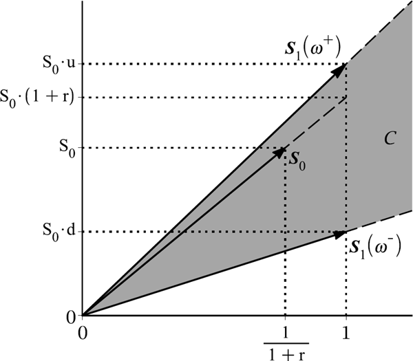
The no-arbitrage condition means that the initial price vector S0 has to lie inside the cone C ⊂ ℝ+N generated by the M column vectors of the payoff matrix D. This situation is illustrated in the case where M = N = 2.
S0d<(1+r)S0<S0u⇔d<1+r<u.
This criterion can be generalized on any model with two base assets and arbitrarily many states of the world. The vector S0 lies inside the cone C iff
minω∈ΩS2T(ω)S1T(ω)<S20S10<maxω∈ΩS2T(ω)S1T(ω).
5.3.4 Risk-Neutral Probabilities
An important component of Theorem 5.9 is the M-dimensional vector Ψ ≫ 0 which solves D Ψ = S0. As follows from (5.11), the initial value of a portfolio φ ∈ ℝN is equal to the product of the terminal payoff vector and the state-price vector, Πϕ0=ΠϕT(Ω)Ψ. Therefore, the no-arbitrage initial value π0(X) of an attainable payoff X replicated by φX can be calculated as follows:
π0(X)=∏0[ϕX]=M∑j=1∏T[ϕX](ωj)Ψj=M∑j=1X(ωj)Ψj=XΨ. (5.13)
As is seen from (5.13), a replicating portfolio is not required to calculate the no-arbitrage initial value (i.e., the fair price) of a claim with an attainable payoff. We only need to find the vector Ψ and then multiply it by the payoff vector to find π0(X). The solutions Ψj ∈ (0, ∞), j =1, 2,...,M, are called state prices. To explain such a name, consider an Arrow–Debreu security εj=I{ωj} having a nonzero payoff of one unit only for the state ωj. According to (5.13), the initial price of εj is
π0(εj)=M∑k=1εj(ωk)Ψk=M∑k=1I{ωj}(ωk)Ψk=Ψj. (5.14)
Thus, the financial meaning of the solutions Ψj ∈ (0, ∞), j = 1, 2,...,M, is that they are no-arbitrage prices of the Arrow–Debreu securities. In particular, Ψj can also be thought of as the price of an insurance contract that pays one unit of currency in case scenario ωj occurs.
The pricing formula (5.13) can also be derived using (5.14) and the principle of linear pricing. According to Proposition 5.1, every payoff X can be represented as a portfolio in AD securities:
X=x1ε1+x2ε2+⋯+xMεMforsomex1,x2,...,xM∈ℝ.
Thus, the initial value π0(X) is the same as that of the portfolio in the AD securities:
π0(X)=x1π0(ε1)+x2π0(ε2)+⋯+xMπ0(εM)=x1Ψ1+x2Ψ2+⋯+xMΨM=XΨ.
Consider a risk-less asset B that pays one unit of currency at the terminal time (i.e., B is a zero-coupon bond). According to (5.13), since BT (ωj)= 1 for all j = 1,...,M, the initial price of the payoff BT ≡ 1 is
B0:=π0(BT)=M∑j=1Ψj.
Let us set 1+r = (∑Mj=1ψj)−1. Hence B0=11+r. The quantity r is in fact the single-period return on B:
BT−B0B0=BTB0−1=1(1+r)−1−1=r.
Now we are ready to rewrite the security pricing formula (5.13) in a more familiar form.
First, note that the positive state prices Ψj, j = 1, 2,...,M, can be normalized to give us a new set of probabilities:
˜pj:=Ψj∑Mi=1Ψi,j=1,2,...,M. (5.15)
Clearly, all ˜pj's are positive and sum to unity. These probabilities are called risk-neutral probabilities and they have no relation to the real-world (physical) probabilities {pj = ℙ(ωj)}. The real-world probabilities can be estimated from historical data, whereas the risk-neutral probabilities are not observed. Let ˜ℙ denote the risk-neutral probability measure defined by ˜ℙ(ωj)=˜pj for j = 1, 2,...,M. The risk-neutral probability of any event E ⊆ Ω is then given by
˜ℙ(E)=∑ω∈E˜ℙ(ω)=∑ωj∈E˜pj.
The mathematical expectation of a random variable X ∈ℒ(Ω) with respect to ˜ℙ, denoted by ˜E[X], is defined by
˜E[X]=M∑j=1X(ωj)˜pj.
Using (5.15), the initial price in (5.13) can now be written as the mathematical expectation of the discounted payoff function with respect to the risk-neutral probability measure:
π0(X)=M∑j=1X(ωj)Ψj=(M∑k=1Ψk)M∑j=1X(ωj)Ψj∑Mk=1Ψk=11+rM∑j=1X(ωj)˜pj=11+r˜E[X]. (5.16)
Here, X1+r is the discounted value of X. That is, it is the present (time-0) value of the payoff paid at time T. If we apply (5.16) to a portfolio that only contains one unit of the base asset Si, then we have that
Si0=11+r˜E[SiT]. (5.17)
Therefore, the risk-neutral expectation of the return on Si is
˜E[SiT−Si0Si0]=˜E[SiT]Si0−1=(1+r)−1=r.
In other words, in the risk-neutral probability measure, the expected return of any base security is equal to the risk-free interest rate r on the bond B. Since B0/BT = (1 + r)−1, we can rewrite (5.17) as
Si0B0=˜E[SiTBT] (5.18)
for every base asset Si ,i = 1,...,N. In other words, the discounted asset price processes {ˉSit:=SitBt}t∈{0,T}, i = 1, 2,...,N, are martingales under the risk-neutral probability measure ˜ℙ. The subject of martingales will be introduced and covered in depth in the next chapter. It suffices to note here that the discounted price processes {ˉSit}t∈{0,T} are examples of single-period stochastic processes. A single-period stochastic process, say {Xt}t∈{0,T}, is a called a martingale with respect to the measure ˜ℙ if ˜E(XT)=X0. That is, our best prediction of the future time-T value (i.e., the expected future value with respect to the given measure) of the process is the same as the current time-0 value.
To summarize, if the single-period market model is arbitrage-free, then there exists a risk-neutral probability measure ˜ℙ. Conversely, we can construct a state-space vector from the risk-neutral probabilities as
Ψj=˜pj1+r,j=1,2,...,M.
Hence, the existence of ˜ℙ implies no arbitrage. Therefore, Theorem 5.9 can now be formulated as follows.
Theorem 5.10
(The first FTAP—the 2nd version). There are no arbitrage portfolios in a single-period N-by-M model iff there exist probabilities {˜pj>0:j=1,2,...,M} such that the discounted asset price processes {ˉSit}t∈{o,T}, i = 1, 2,..., N, are all martingales with respect to the probability measure ˜ℙ. Such a probability measure is called the risk-neutral probability measure.
Let us come back to the binomial model from Example 5.1 with two states and two assets: St1 = Bt and St2 = St. We readily solve for the state-price vector as follows:
[11S0uS0d][Ψ1Ψ2]=[(1+r)−1S0]⇔{Ψ1+Ψ2=11+ruΨ1+dΨ2=1 ⇔{Ψ1=(1+r)−d(1+r)(u−d)Ψ2=u−(1+r)(1+r)(u−d) (5.19)
The solution Ψ = [Ψ1, Ψ2]Τ in (5.19) is strictly positive iff d < 1 + r < u. If 1 + r ≤ d, then an arbitrage portfolio can be obtained by shorting the bond (for example, φ1 = −S0(1 + r) and φ2 = 1). If 1 + r ≥ u, then an arbitrage portfolio can be obtained by shorting the stock (for example, φ1 = S0(1 + r) and φ2 = −1). The reader may verify that Π0φ is zero and ΠTφ is positive in both cases. Finally, we can calculate the risk-neutral probabilities for the binomial model:
˜p≡˜p1=Ψ1Ψ1+Ψ2=(1+r)−du−d,1−˜p≡˜p2=Ψ2Ψ1+Ψ2=u−(1+r)u−d.
The probabilities are strictly positive iff the no-arbitrage condition d < 1+ r < u holds. Finally, note that the state prices are themselves given by the discounted (risk-neutral) expected value of the Arrow–Debreu payoffs:
Ψj=11+r˜E[εj],j=1,...,M.
5.3.5 The Second Fundamental Theorem of Asset Pricing
We are now ready to present the second fundamental theorem of asset pricing which states a sufficient and necessary condition of completeness of a market model. We give two versions of the theorem: first in terms of state prices and then in terms of risk-neutral probabilities.
Theorem 5.11
(The second FTAP). Assuming absence of arbitrage, there exists a unique solution to the state-price equation, Ψ ≫ 0, iff the market is complete.
(The second FTAP—the 2nd version). Assuming absence of arbitrage, there exists a unique set of risk-neutral probabilities {˜pj>0:j=1,2,...,M} iff the market is complete.
Proof. The no-arbitrage assumption implies that there exists a strictly positive solution Ψ to the matrix equation D Ψ = S0. If the market is complete, then rank(D) = M. Hence the solution is unique. Conversely, let the solution Ψ ≫ 0 be unique. We will argue that the market is complete by contradiction. If the market is not complete, then rank(D) < M. Therefore, there exists a nontrivial solution λ ≠ = 0 to the matrix equation D λ = 0. Since Ψj > 0 for all 1 ≤ j ≤ M, there exists a sufficiently small constant a ≠ 0 such that Ψj + aλj > 0 for all 1 ≤ j ≤ M, i.e., Ψ + aλ ≫ 0. Moreover, this vector solves
D(Ψ+aλ)=DΨ+aDλ=S0+a0=S0.
Thus, Ψ + aλ is another state-price vector. This contradicts our hypothesis that the state-price vector is unique.
Example 5.7.
Verify if the single-period model from Example 5.6 is complete.
Solution. In cases (a) and (b), there exists a positive solution to the state-price equation DΨ = S0. Hence, there are no arbitrage opportunities. In case (a), the solution Ψ is unique; therefore, the model is complete. In case (b), there are infinitely many positive solutions parametrized by t∈(0,14); therefore, the model is incomplete. Indeed, in case (b) the determinant of the payoff matrix is zero; hence, the model is incomplete. For example, the payoff of the at-the-money call option on asset S2 is unattainable since the system φ D = [0, 0, 2] is inconsistent.
5.3.6 Investment Portfolio Optimization
A no-arbitrage price of a derivative security is calculated by taking the risk-neutral expectation of the payoff function. So, a model that does not admit arbitrage opportunities has two probability measures, the actual (real-world) measure and the risk-neutral measure. We only use the latter in no-arbitrage pricing. As is demonstrated in previous chapters, the real-world measure is used in asset management and risk management. However, as is shown below, the risk-neutral measure also plays an important role when finding an optimal allocation.
Consider the following investment problem for a nonarbitrage, complete model. Being given an initial capital W0, we find a portfolio φ = ℝN with initial value Π0φ = W0 that maximizes the expected utility of the terminal value, E[u(ΠTφ)], where u is a utility function, i.e., u is a nondecreasing and concave function. That is, we find the solution to the following constrained optimization problem:
max imizeE[u(∏ϕT)]=M∑j=1u(∏ϕT(ωj))pj=M∑j=1u(N∑i=1ϕiSiT(ωj))pjw.r.tϕ∈ℝN (5.20)
subjectto∏ϕ0=N∑i=1ϕiSi0=W0. (5.21)
Since the market model is complete, the solution of the problem (5.20)–(5.21) can be split into two steps: first, we find the terminal value of the optimal portfolio ΠTφ, i.e., a (terminal) payoff X, that maximizes the expected utility E[u(X)]; second, we find the optimal portfolio vector φ that replicates the payoff X. To obtain a constraint equation on X, we use the fact that the discounted value process is a martingale under the risk-neutral probability measure:
11+r˜E[∏ϕT]=∏ϕ0=W0.
Denoting X = ΠTφ and using state prices gives
11+r˜E[X]=11+rM∑j=1xj˜pj=M∑j=1xjΨj=W0.
The optimization problem (5.20)–(5.21) now takes the form
E[u(X)]=M∑j=1u(xj)pj→maxx∈ℝM (5.22)
subjecttoXΨ=M∑j=1xjΨj=W0. (5.23)
Here, X = [x1, x2,...,xM] denotes the payoff vector for X ∈ ℒ(Ω), i.e., X(ωj)= xj for all j =1, 2,..., M. Let X* be a solution to (5.22)–(5.23). Solving the matrix-vector equation ΠTφ = X* gives the optimal portfolio φ*. Under the completeness assumption, the solution φ* exists and is unique.
Example 5.8.
Consider a single-period model with two scenarios {ω+,ω−} and two base assets, namely, a risky stock with prices ST (ω+) = 12, ST (ω−) = 8, S0 = 10, and an atthe-money call option on the stock with initial price C0 = 1. Suppose that the real-world probabilities are p=ℙ(ω+)=14 and 1−p=ℙ(ω−)=34. Find the optimal portfolio (φ1, φ2) with initial value W0 = 100 that maximizes E[√ΠT[(ϕ1,ϕ2)]].
Solution. The strike price of the call option is K = S0; the payoff is CT (Ω) = (ST (Ω) − S0)+ = [2, 0]. Hence, the initial price vector and payoff matrix are, respectively, given by
S0=[101],D=[12820].
Solving the matrix-vector equation, D Ψ = S0 for Ψ = [Ψ1, Ψ2]Τ, gives the state prices Ψ1=Ψ2=12.
First, we find the payoff vector X = [x1, x2] that solves the optimization problem
E[√X]=14√x1+34√x2→max x1,x2subjecttox1Ψ1+x2Ψ2=x1+x22=100.
The optimal value of x1 is a point of maximum of the function
f(x)=14√x+34√200−x.
Equating the derivative f′(x)=18√x−38√200−x to zero and solving the equation obtained gives the solution x = 20. Since the second derivative f″(x) is strictly negative for all x ∈ (0, 200), the function f attains its maximum at x = 20. Thus, the terminal payoff of the optimal portfolio is given by
x1=20andx2=180.
The Profit&Loss realized is X − W0, which is equal to −80 in state ω+ and 80 in state ω−.
Second, find portfolio [φ1, φ2] replicating the payoff X = [20, 180]. Solve the system of replication equations:
{12ϕ1+2ϕ2=208ϕ1+0ϕ2=180⇒{ϕ1=452ϕ2=−125
So, the optimal allocation portfolio is [ϕ1,ϕ2]=[452,−125]. This means that we should sell 125 call contracts and purchase 22.5 units of stock.
To find a general solution to the optimization problem (5.22)–(5.23), we apply the method of Lagrange multipliers. The Lagrangian is
L(X,λ)=M∑j=1u(xj)pj−λ(M∑j=1xjΨj−W0).
Differentiating L w.r.t. x1, x2,...,xM, and λ, and equating the derivatives obtained to zero gives the following simultaneous equations:
∂L∂xj=u′(xj)pj−λΨj=0,j=1,2,...,M, (5.24)
∂L∂λ=W0−M∑j=1xjΨj=0. (5.25)
Suppose that the derivative of the utility function, u′, is strictly monotone, i.e., it is a strictly increasing function everywhere it is finite. Additionally, we assume that the range of possible values of u′(x) includes all positive reals. Examples of such utility functions include ln x and xγ with γ ∈ (0, 1). Under the above assumptions, the equation u′(x) = y has a unique solution for every y ∈ (0, ∞). Thus, we can define the inverse function v for u′ with the property that u′(v(y)) = y for all y ∈ (0, ∞).
Now, solving the equations in (5.24) individually gives
xj=v(λΨjpj),j=1,2,...,M. (5.26)
So, we have a formula for the optimal payoff in terms of the multiplier λ. Substituting (5.26) into (5.25) gives
M∑j=1ν(λΨjpj)Ψj=W0. (5.27)
Solving (5.27) for λ and substituting the solution λ* into (5.26) gives the optimal payoff vector
x*j=ν(λ*Ψjpj),j=1,2,...,M. (5.28)
Let us show that the solution X* with values in (5.28) maximizes E[u(X)]. That is, let us show that for every payoff X ∈ ℒ(Ω) chosen such that π0(X) = X Ψ = W0 we have
E[ν(X)]≤E[ν(X*)].
Consider the function f(x) := u(x) − yx with a positive parameter y. Clearly, x = v(y) maximizes f. Indeed, solving f′(x) = u′(x) − y = 0 gives x = v(y); since f″(x) = u″(x) ≤ 0 for all x, x = v(y) is a point of maximum. Therefore, we have
ν(x)−yx≤ν(ν(y))−yν(y)forallx. (5.29)
Replacing x and y in (5.29) by xj and λ*Ψjpj, respectively, multiplying both parts of the inequality by pj, and then using (5.28) gives
ν(xj)pj−λ*Ψjxj≤ν(x*j)pj−λ*Ψjxjforallj=1,2,...,M.
Adding all the above M inequalities up gives
M∑j=1ν(xj)pj−λ*M∑j=1Ψjxj≤M∑j=1ν(x*j)pj−λ*M∑j=1Ψjx*j.
This is equivalent to
E[ν(X)]−λπ0(X)≤E[ν(X*)]−λπ0(X*).
Since the payoffs X and X* have the same initial value equal to W0, we obtain that E[u(X)] ≤ E[u(X*)]. That is, X* maximizes E[u(X)] and hence it is the payoff of the optimal portfolio. Finally, note that the difference X*(ωj) − W0 is the actual gain (if positive) or loss (if negative) realized in state ωj. Under the no-arbitrage condition, the gain X − W0 (if it is not identically zero) has to change its sign: to be negative in at least one state and positive in another state.
Example 5.9.
Consider a 3-by-3 model with
D=[11116151286]andS0=[1510].
Suppose that the real-world-probabilities are p1=p3=14 and p2=12. Find the optimal portfolio φ that maximizes E[ln(ΠT [φ])] and has initial value W0 = 1. Find the gain/loss realized.
Solution. By solving D Ψ = S0, we obtain the state-price vector Ψ=[813,213,313]Τ. It is strictly positive and unique, hence the model is arbitrage-free and complete. The utility function u(x) = ln x satisfies the criteria stated above since the derivative u′(x)=1x varies from 0 to ∞ as x ↗ ∞ and x ↘ 0, respectively. Substituting the inverse of the derivative, υ(y)=1y, into (5.28) gives the optimal payoff X* in terms of λ*:
xj=pjλ*Ψj,j=1,2,3⇒X*=1λ*[1332,134,1312].
Solving (5.27) with W0 = 1 for λ gives
1=3∑j=1pjλΨjΨj=1λ3∑j=1pj=1λ⇒λ*=1.
Therefore, the optimal payoff vector is X*=[1332,134,1312]. Solving the matrix-vector equation φ D = X* gives the optimal allocation portfolio:
ϕ*=[85348,−5396,−269192].
The gain of the investment is X*−W0=[−1932,94,112]. So the return on the investment is only positive in states ω2 and ω3.
5.4 Pricing in an Incomplete Market
5.4.1 A Trinomial Model of an Incomplete Market
The simplest single-period incomplete market model is a model with three states of the world, i.e., Ω = {ω1,ω2,ω3}≡{ω+,ω0,ω−}, and two assets: B and S. The risk-free asset B provides the rate of return r and it pays $1 at maturity:
B0=11+r,BT=1.
The risky asset S admits three possible cash flows at time T :
ST(ω)={S0uifω=ω1,S0mifω=ω2,S0difω=ω3,
where S0 > 0 is the initial price and 0 < d < m < u are price factors. The initial price vector and the cash-flow matrix are, respectively, given by
S0=[(1+r)−1S0]andD=[BT(ω1)BT(ω2)BT(ω3)ST(ω1)ST(ω2)ST(ω3)]=[111S0uS0mS0d].
D has rank 2 since |11S0uS0m|=S0(m−u)≠0. The two payoff vectors [1, 1, 1] and [S0u, S0m, S0d] are clearly independent. Therefore, we conclude that there are no redundant base assets but the market is incomplete as the two vectors do not span ℝ3. We wish to find all strictly positive solutions Ψ to the equation D Ψ = S0. This is a linear system of two equations and three unknowns. Generally, the solution represents a line in ℝ3 corresponding to the intersection of two planes:
{Ψ1+Ψ2+Ψ3=(1+r)−1uΨ1+mΨ2+dΨ3=1⇔{Ψ1=(1+r)−d(1+r)(u−d)−m−du−dcΨ2=cΨ3=u−(1+r)(1+r)(u−d)−u−mu−dc (5.30)
We set c > 0, giving Ψ2 > 0. The limiting value of Ψ as c ↘ 0 is
Ψ2↘0,Ψ1↗(1+r)−d(1+r)(u−d),andΨ3↗u−(1+r)(1+r)(u−d).
The limiting values of Ψ1 and Ψ3, as c ↘ 0, are strictly positive iff d < 1+ r < u holds. Therefore, there exists a strictly positive solution Ψ=[Ψ1,Ψ2,Ψ3]Τ iff d < 1 + r < u. Indeed, if 1 + r ≤ d, then Ψ1 < 0 for any Ψ2 = c > 0; if u ≤ 1 + r, then Ψ3 < 0 for any Ψ2 = c > 0. From (5.30), we obtain all values of c such that Ψj > 0, j = 1, 2, 3:
Ψ1>0⇔c<(1+r)−d(1+r)(m−d),Ψ2>0⇔c>0,Ψ3>0⇔c<u−(1+r)(1+r)(u−m).
Thus, the solution Ψ = Ψ(c) from (5.30) is strictly positive iff
c∈(0,cmax ),wherecmax :=11+rmin {(1+r)−dm−d,u−(1+r)u−m}.
Such a set of positive solutions, denoted by {Ψ}, is an open segment of a line in ℝ3 . Indeed, according to (5.30), Ψ(c) is a linear function of c. Hence all solutions lie on a straight line. Since 0 ≤ Ψj ≤ (1+r)−1 for j = 1, 2, 3, the set {Ψ} is bounded. The coordinates of the two endpoints of {Ψ}, denoted by Ψ(0) and Ψ(cmax) are obtained by setting c = 0 and c = cmax in (5.30), respectively:
Ψ(0)=[(1+r)−d(1+r)(u−d),0,u−(1+r)(1+r)(u−d)]Τ, (5.31)
Ψ(cmax )={[(1+r)−m(1+r)(u−m),u−(1+r)(1+r)(u−m),0]Τ,ifm≤1+r,[0,(1+r)−d(1+r)(m−d),m−(1+r)(1+r)(m−d)]Τ,ifm≥1+r. (5.32)
All the solutions of {Ψ} can be parametrized as Ψ(v cmax) = (1−v)Ψ(0)+vΨ(cmax), where υ=ccmax ∈(0,1).
The binomial model (with two states) is recovered as a limiting case of the trinomial model as Ψ2 → 0. By setting c = 0 in (5.30), we obtain
Ψ1=(1+r)−d(1+r)(u−d),Ψ2=0,Ψ3=u−(1+r)(1+r)(u−d).
The formulae of the state prices Ψ1 and Ψ3 are exactly the same as those of the binomial state prices in (5.19). Two other extreme cases are obtained by setting either Ψ1 or Ψ3 to zero:
- Let Ψ1 ↘ 0. Then Ψ3=11+rm−(1−r)m−d and Ψ2=11+r(1+r)−dm−d. If d < 1+ r < m, then both Ψ2 and Ψ3 are positive.
- Let Ψ3 ↘ 0. Then Ψ1=11+r(1+r)−mu−m and Ψ2=11+ru−(1+r)u−m. If m < 1 + r < u, then both Ψ1 and Ψ2 are positive.
Alternatively, one can recover the binomial model in the limiting case as m ↘ d or m ↗ u.
For every positive state-price vector Ψ ∈ {Ψ} we can identify a respective risk-neutral probability measure with the probabilities ˜pj=(1+r)Ψj,j=1,2,3. Therefore, any incomplete arbitrage-free model has infinitely many risk-neutral probability measures. For the trinomial model described above, the collection of risk-neutral probability measures (i.e., the probability mass functions) can be denoted as vectors ˜p=[˜p1,˜p2,˜p3], forming an open linear segment in ℝ3, whose endpoints are
˜Ρ(0)=(1+r)Ψ(0)and˜Ρ(cmax )=(1+r)Ψ(cmax ). (5.33)
Hence, we have a collection of risk-neutral measures and risk-neutral probability vectors that we denote by {˜ℙ} and {˜p}, respectively.
Consider a single-period trinomial model with two assets B and S where S0 = $100, d =0.8, m =1.1, u = 1.4, r = 0.2. Show that the model is arbitrage-free. Find all strictly positive state-price vectors and risk-neutral probability vectors.
Solution. The initial price vector and payoff matrix are, respectively,
S0=[56100]andD=[11114011080].
Let us find the general solution to the state-price equation D Ψ = S0:
[11114011080|56100]~[11200121|59518]⇒{Ψ1=59−c2,Ψ2=c,Ψ3=518−c2.
The state-price vector
Ψ(c)=[59−c2,c,518−c2]Τ (5.34)
is strictly positive iff 0<c<59. Therefore, there is no arbitrage. Alternatively, we can notice the condition d < 1 + r < u is satisfied and hence the model is arbitrage-free.
Now, we find the risk-neutral probabilities. Applying (5.31)–(5.32) and (5.33) gives the following endpoints of the collection of risk-neutral probability vectors {˜p}:
˜Ρ(0)=[(1+r)−du−d,0,u−(1+r)u−d]Τ=[1.2−0.81.4−0.8,0,1.4−1.21.4−0.8]Τ=[23,0,13]Τ,˜Ρ(59)=[(1+r)−mu−m,u−(1+r)u−m,0]Τ=[1.2−1.11.4−1.1,1.4−1.21.4−1.1,0]Τ=[13,23,0]Τ.
The collection {˜p} of risk-neutral probability vectors can be parametrized by a single variable as follows:
˜Ρ(5ν9)=(1−ν)˜Ρ(0)+ν˜Ρ(59)=[2−ν3,2ν3,1−ν3]Τ,ν∈(0,1). (5.35)
Alternatively, the solution (5.35) can be obtained by normalizing the state-price vector in (5.34) and applying the change of variables c=59υ:
Ψ(c)∑3j=1Ψj(c)=[23−3c5,6c5,13−3c5]Τ=[2−ν3,2ν3,1−ν3]Τ,ν∈(0,1).
5.4.2 Pricing Nonattainable Payoffs: The Bid-Ask Spread
Assume that the Law of One Price holds. Then the no-arbitrage initial price of any financial claim with an attainable payoff is unique and is given by the initial value of any portfolio in the base assets that replicates the payoff. We can use (5.13) to price an attainable payoff X in the trinomial model. Alternatively, the pricing formula in (5.16) is used with the risk-neutral probabilities ˜pj=(1+r)Ψj,j=1,2,3. Any choice of state-price vector Ψ, or the corresponding risk-neutral probability measure ˜ℙ, gives us the same value for the initial price π0(X).
Example 5.11.
Consider the trinomial model from Example 5.10. Find the no-arbitrage initial price of a long forward contract F with the delivery (strike) price K = $100.
Solution. The payoff of a long forward contract is attainable as it is replicated by a portfolio consisting of one long position in the stock and a loan in the amount of K:
FT:=ST−K=ST−KBT.
The initial price F0 of the forward contract is unique and equal to
F0=S0−KB0=S0−K1+r=100−1001.2=503≅$16.67.
On the other hand, we know that the risk-neutral pricing formula (5.16) must give us the same initial value of the contract regardless of the choice of the risk-neutral probability measure ˜ℙ(c) with c∈(0,59). Using the probabilities in (5.35) gives
F011+rE˜ℙ(c)[FT]=11+r3∑j=1(ST(ωj)−K)˜pj(c)=11.2((80−100)⋅1−ν3+(110−100)⋅2ν3+(140−100)⋅2−ν3)=−20(1−ν)+20ν+40(2−ν)3.6=−20+20ν+20ν+80−40ν3.6=603.6=503≅$16.67,
where υ=9c5∈(0,1). Alternatively, using the pricing formula (5.13) and solution (5.34) gives
F0=3∑j=1FT(ωj)Ψj(c)=(−20)⋅(518−c2)+10⋅c+40⋅(59−c2)=(10+10−20)c+200−509=503.
To price a nonattainable payoff, we can formally apply (5.13), or equivalently the asset pricing formula in (5.16). However, the no-arbitrage initial price of X∉A(Ω) is now not unique since there are infinitely many no-arbitrage state-price vectors Ψ, or equivalently infinitely many risk-neutral measures. There are several approaches to deal with incomplete market models. One approach is to complete the market by including extra tradeable securities into the market model for which the initial value is known. It should be evident that the additional security should not be a redundant one as this would not change the original space of attainable payoffs. For example, we can add in some other security such as an option on the underlying risky asset or stock with known market value. We now give an example of how this is accomplished.
Consider the incomplete trinomial model from Example 5.10.
- (a) Show that the payoff of the European call option with strike K = $100 is nonattainable.
- (b) Assume that the initial price of the call option from (a) is $20. Add this option in the trinomial model as a third base asset. Show that the new model with three base assets is complete and arbitrage-free.
(a) First, calculate the values of the European call payoff X = (ST − K)+:
X(ω1)=(ST(ω1)−K)+=(140−100)+=40,X(ω2)=(ST(ω2)−K)+=(110−100)+=10,X(ω3)=(ST(ω3)−K)+=(80−100)+=0.
Second, we try to replicate X by a portfolio in B and S. That is, find (if possible) a portfolio vector φ ∈ ℝ2 such that
ϕD=X⇔{ϕ1+140ϕ2=40ϕ1+110ϕ2=10ϕ1+80ϕ2=0 (5.36)
The rank of the augmented coefficient matrix of the system in (5.36) is 3 and hence is not equal to rank(D) = 2 since
|1140401110101800|=−600≠0.
Therefore, the system of linear equations in (5.36) is inconsistent, i.e., it does not have a solution.
(b) Now assume that the European call is the third base asset. The initial price vector and payoff matrix of the new 3-by-3 model are, respectively,
ˆS0=[5610020]andˆD≡ˆST(Ω)=[1111401108040100].
The payoff matrix ˆD has a full rank so the 3-by-3 model does not have redundant assets and is complete. To prove the absence of arbitrage, we need to show that the solution Ψ to the linear system ˆDΨ=ˆS0 is strictly positive. Find Ψ as follows:
{Ψ1+Ψ2+Ψ3=56140Ψ1+110Ψ2+80Ψ3=10040Ψ1+10Ψ2+0Ψ3=20⇔{Ψ1=49Ψ2=29Ψ3=16
As we can see, the state-price vector Ψ=[49,29,16]Τ is strictly positive. Therefore, the 3-by-3 model is arbitrage-free. The risk-neutral probabilities are
˜Ρ1=(1+r)Ψ1=815,˜Ρ2=(1+r)Ψ2=415,˜Ρ3=(1+r)Ψ3=15.
Another approach to pricing a security with an unattainable payoff X is to find two attainable payoffs Xd and Xu so that Xd(ω) ≤ X(ω) ≤ Xu(ω) for all ω ∈ Ω. Then, the no-arbitrage price π0(X) is bounded:
π0(Xd)<π0(X)<π0(Xu).
Indeed, let the portfolios φd and φu replicate Xd and Xu, respectively. Suppose that π0(Xd) ≥ π0(X), then there exists the following arbitrage opportunity. At time t = 0 we buy the security and sell the portfolio φd. Our proceeds, which we keep in cash, are nonnegative:
∏0[ϕd]−π0(X)=π0(Xd)−π0(X)≥0.
At time t = T the net position is nonnegative in all states and strictly positive in some states:
X−∏T[ϕd]=X−Xd>0.
Indeed, since Xd≤X,Xd∈A(Ω), and X∉A(Ω), we have that Xd(ω) < X(ω) in at least one state ω. Hence, this is an arbitrage portfolio with a positive payoff equal to (π0(Xd) − π0(X)) + X − Xd. Similarly, there would be an arbitrage opportunity if the security with payoff X were found to be selling in the market at a price π(X) ≥ π0(Xu).
A super-replicating portfolio φ with the terminal value
∏ϕT≥X (5.37)
covers the liabilities of the writer of the security with payoff X. So the writer will choose φ with minimal initial cost Π0φ subject to the constraints (5.37). As a result, the writer obtains the following linear programming problem (the super-replication problem):
∏ϕ0→minϕ∈ℝNsubjectto∏ϕT≥X. (5.38)
Since the risk-free security is strictly positive, the linear programming problem is feasible. There always exists a risk-free portfolio that satisfies the constraints (5.37). The problem (5.38) is equivalent to the minimization of π0(Y) over the set of dominating attainable claims for X:
π0(Y)→min Y∈DX,whereDX:={Y∈A(Ω):X≤Y}. (5.39)
The set DX≠φ includes all payoffs that dominate the claim's payoff X.
The problem (5.38) or (5.39) can be solved graphically or numerically. Let us denote the optimal solution to (5.38) by φu . Then π0u(X) := Π0[φu] is an upper bound for a no-arbitrage initial price π0(X) for the derivative or claim with payoff X. If the writer were selling the security at a price higher than π0 u(X), then another agent could form an arbitrage portfolio.
Let us now look at the matter from the buyer's perspective. Let the portfolio φ = φd solve the linear programming problem (the sub-replication problem):
∏ϕ0→max ϕ∈ℝNsubjectto∏ϕT≤X. (5.40)
The problem (5.40) is equivalent to the maximization of π0(Y) over the set of attainable claims dominated by X:
π0(Y)→max Y∈ℳX,whereℳX:={Y∈A(Ω):Y≤X}. (5.41)
The set ℳX≠φ includes all payoffs that are dominated by the claim's payoff X. Denote the initial value of the portfolio φd by π0d(X). The buyer of the derivative security with payoff X will not agree to pay more than π0d(X) since it will be more beneficial to purchase the portfolio in base assets rather than the derivative. As a result we obtain a lower bound for a no-arbitrage price of π0(X). In summary, the initial price π0(X) for the claim with payoff X must satisfy the inequality relation
πd0(X)<π0(X)<πu0(X). (5.42)
Otherwise, an arbitrage opportunity will arise. The interval π0d(X),π0u(X) is called the bid-ask spread for the initial price of a derivative security with payoff X.
The ask price π0u(X) and the bid price π0d(X) can also be calculated by respectively taking the maximum and the minimum of the discounted expectation of the payoff function over the set of possible risk-neutral measures:
πu0(X)=supℙ˜∈{˜ℙ}{11+rM∑i=1˜piX(ωi)}=supΨ∈{Ψ}XΨ, (5.43)
πd0(X)=infℙ˜∈{˜ℙ}{11+rM∑i=1˜piX(ωi)}=infΨ∈{Ψ}XΨ. (5.44)
Here, {Ψ} and {˜ℙ} denote the collection of no-arbitrage state-price vectors and the corresponding collection of risk-neutral probabilities measures, respectively.
Consider the case of the trinomial model. State-price vectors form a finite segment in ℝ3. Thus, the range of possible no-arbitrage initial prices of a nonattainable payoff is also a finite segment. Since the price π0 = X Ψ is a linear function of the vector Ψ, these bounds are attained at the endpoints (5.31)–(5.32) of the state-price set {Ψ}.
Example 5.13.
Consider the trinomial (incomplete) model from Example 5.10. Find the bid-ask spread for the initial price of the call option with strike K = $100.
Solution. The first approach is to solve the super-and sub-replication problems given by (5.38) and (5.40), respectively,
{∏0[ϕd]→max ϕd∈ℝ2∏T[ϕd]≤X⇔{56ϕd1+100ϕd2→max [ϕd1,ϕd2]∈ℝ2ϕd1+80ϕd2≤0,ϕd1+110ϕd2≤10,ϕd1+140ϕd2≤40 (5.45)
{∏0[ϕu]→min ϕu∈ℝ2∏T[ϕu]≤X⇔{56ϕu1+100ϕu2→min [ϕu1,ϕu2]∈ℝ2ϕu1+80ϕu2≤0,ϕu1+110ϕu2≤10,ϕu1+140ϕu2≤40 (5.46)
The solutions to the linear programming problems (5.45) and (5.46) are, respectively,
ϕd=[−100,1]andϕu=[−5313,23].
The bid price π0d and ask price π0u of the call option are then given by
πd0=∏0[ϕd]=−100⋅56+1⋅100=503≅$16.67,πu0=∏0[ϕu]=−5313⋅56+23⋅100=2009≅$22.22.
Thus, the bid-ask spread is (16.67, 22.22).
The other approach is to find the bid-ask spread by computing the extreme values of the risk-neutral expectation of the discounted payoff. Since the mathematical expectation of a random variable from ℒ(Ω) is a linear function of the state probabilities, the maximum and minimum in (5.43) and (5.44) are attained at the endpoints of the domain {˜ℙ}. Therefore, we just need to calculate the expected value
π0(c)=11+rE˜ℙ(c)[(ST−K)+]=11+r3∑j=1˜pj(c)(ST(ωj)−K)+
using risk-neutral probabilities given by (5.35) with extreme values c = 0 and c=59. The bid price is the smaller of the two prices calculated, and the ask price is the larger one. The above expectation is calculated explicitly in the measure ˜ℙ(υ):
π0(5ν9)=56⋅(0⋅1−ν3+10⋅2ν3+40⋅2−ν3)=50(4−ν)9,0≤ν≤1.
The extreme values are π0(υ=0)=2009 and π0(υ=1)=503=1509. The bid price is min {2009,503}=503, and the ask price is max {2009,503}=2009. As required, both prices agree with the values obtained using the first approach.
In the conclusion of this section, let us consider an example of a single-period model with four states of the world and two tradable assets.
Example 5.14.
Let the initial price vector and payoff matrix be given by
S0=[1010]andD=[11111111681214].
- (a) Show that the market is arbitrage-free. Find the general solution for the state prices and illustrate it with a diagram.
- (b) Find the bid-ask spread for the put option on the risky asset with strike price K = 11.
Solution. The general solution to the state-price equation D Ψ = S0 is a function of two free parameters:
{Ψ1=2x+3y−1511Ψ2=2511−3x−4yΨ3=xΨ4=y
The solution is strictly positive if
0<x<2533andmax {511−23x,0}<y<2444−34x (5.47)
holds. The domain of admissible solutions, D = {[x, y]: Ψ(x, y) ≫ 0}, can be illustrated by a diagram on the (x, y)-plane (Figure 5.3).

The no-arbitrage initial price π0 of the put option with strike price K = 11 is given by a product of the payoff vector
Ρ=(K−S(Ω))+=[5,3,0,0]
and the state-price vector Ψ:
π0=ΡΨ=5⋅(2x+3y−1511)+3⋅(2511−3x−4y)=x+3y.
The bid and ask prices are, respectively, the minimum and maximum values attained by the function x + 3y in the domain D as is specified in (5.47). These values can be found by solving respective linear programming problems. Alternatively, we can use the fact that a linear function attains its extreme values at the boundary. The boundary of the domain D is piecewise linear. Hence, by applying the same principle one more time, we can conclude that the maximum and minimum values of x + 3y in D are attained at the corner points
q1=[0,1533],q2=[0,2544],q3=[1522,0],q4=[2533,0].
Calculate the value of π0 at each of these points:
π0(q1)=1511,π0(q2)=7544,π0(q3)=1522,π0(q4)=2533.
The smaller price is the bid price; the larger price is the ask price:
mini=1,2,3,4,π0(qi)=1522≅0.68182,maxi=1,2,3,4π0(qi)=7555≅1.70455.
Thus, the bid-ask spread for the put option is (0.68182, 1.70455).
5.5 Change of Numéraire
5.5.1 The Concept of a Numéraire Asset
Suppose that there exists a risk-free asset {Bt}t∈{0,T} with a fixed rate of return r. Note that for a risk-free bond we assume nonnegative interest rates so that r ≥ 0. As was shown in the previous section, the market model is arbitrage-free iff there exists a probability function ˜ℙ called a risk-neutral probability measure or martingale probability measure such that the discounted price processes {SitBt}t∈{0,T} for i = 1, 2,..., N are martingales with respect to ˜ℙ.
As a process, the prices of base assets divided by the value of the risk-free account are martingales within a risk-neutral probability measure. There is nothing preventing us from also expressing prices of assets relative to another choice of available strictly positively valued security. The security may be any one of the base assets, or any strictly positively valued portfolio in the base assets, or even a derivative security.
A numéraire, or numéraire asset, or accounting unit, denoted {gt}t∈{0,T}, is any strictly positive asset price process, i.e., with payoff gT ≫ 0 and initial price g0 > 0.
Hence, for any numéraire, we have gt(ω) > 0 for all time t ≥ 0 and all outcomes ω ∈ Ω. The numéraire is used for measuring the relative worth of any asset or a portfolio of assets. The ratio process {Stgt}t≥0 is called the value process of asset S discounted by g or relative to g. The ratio Stgt gives the number of units of the numéraire g that can be exchanged for one unit of asset S at time t. For example, in the binomial model both the bond B and stock S can be chosen as a numéraire.
5.5.2 Change of Numéraire in a Binomial Model
Consider a single-period binomial model with two states of the world Ω = {ω+,ω−} and two base securities B and S such that
B0=(1+r)−1,BT=1,ST(ω)=(dI{ω−}(ω)+uI{ω+}(ω))S0,
where 0 < d < u. The market is arbitrage-free and complete if d < 1 + r < u. Let ˜ℙ be a risk-neutral probability measure with ˜p:=˜ℙ(ω+)=(1+r)−du−d and 1−˜p=˜ℙ(ω−)=u−(1+r)u−d. Under ˜ℙ, the base asset price processes discounted by the numéraire g = B are martingales:
˜E[STBT]=S0B0,˜E[BTBT]=1=B0B0.
Moreover, any portfolio [Δ,β] with Δ shares in the stock S and β units of the bond B discounted by the value of asset B is a martingale:
˜E[ΔST+βBTBT]=Δ˜E[STBT]+β˜E[BTBT]=ΔS0B0+β=ΔS0+βB0B0.
In summary, there is no arbitrage in the binomial model iff there exists a martingale probability measure ˜ℙ(B) for the numéraire g = B. The no-arbitrage binomial model is complete, hence ˜ℙ(B) is unique. Is it possible to use the stock price as a numéraire? Is there a unique risk-neutral probability function ˜ℙ(S) for the numéraire g = S under which the price processes for all base assets are martingales? Both questions are answered positively just below. There exists ˜ℙ(B) with bond B as numéraire iff there exists ˜ℙ(S) with stock S as numéraire. The value process of any attainable claim discounted by numéraire g = B or g = S is a martingale under ˜ℙ(B) or ˜ℙ(S), respectively. Thus, these probability measures are called martingale measures.
The martingale probability measures ˜ℙ(B) and ˜ℙ(S) are said to be equivalent. That is, any event E with zero probability under one measure has zero probability under the other equivalent measure, i.e., ˜ℙ(B)(E)=0 iff ˜ℙ(S)(E)=0 for all E ⊆ Ω. So, two equivalent measures are consistent in their assignment of nonzero probability values to all events having nonzero probability, although the probability values assigned to the events will generally differ. Hence, both ˜ℙ(B) and ˜ℙ(S) are called equivalent martingale measures. The formal definition of equivalent martingale measures in the context of multiple base assets within the single-period setting is given in the next section. Note that the martingale measures ˜ℙ(B) and ˜ℙ(S) and the real-world measure ℙ are equivalent to each other; however, ℙ is not an equivalent martingale measure!
For the binomial case, we only need to show that there exists probability ˜p=˜ℙ(B)(ω+)∈(0,1) iff there exists probability ˜q=˜ℙ(S)(ω+)∈(0,1). Let us work out the martingale probability function ˜ℙ(S). In this case the numéraire asset price at time t is the stock price, gt ≡ St. Hence, the stock price process discounted by gt is a constant and hence is automatically a martingale, i.e., Stgt≡StSt≡1,t∈{0,T}. The bond price BT discounted by ST is given by
BT(ω)ST(ω)=(1+r)B0ST(ω)={1+rdB0S0ifω=ω−,1+ruB0S0ifω=ω+.
So we have that ˜E(S)[BTST]=B0S0 iff
1+ruB0S0˜q+1+rdB0S0(1−˜q)=B0S0⇔1+ru˜q+1+rd(1+˜q)=1.
Here ˜E(S)[⋅] denotes the mathematical expectation under the probability ˜ℙ(S). Solving the above equation for ˜q:
(1+ru−1+rd)˜q=1−1+rd⇔(1+r)(u−d)ud˜q=(1+r)−dd⇔˜q=(1+r)−du−du1+r
The probability measure ˜ℙ(S) is defined by the probabilities ˜q and 1−˜q, which can be expressed in terms of the probabilities for measure ˜ℙ(B),˜p=(1+r)−du−d and 1−˜p, as follows:
˜q=(1+r)−du−d⋅u1+r=˜p⋅u1+r,1−˜q=u−(1+r)u−d⋅d1+r=(1−˜p)⋅d1+r.
Clearly, ˜q ∈ (0, 1) iff d < 1+ r < u. The latter condition is equivalent to ˜p ∈ (0, 1). So assuming no-arbitrage, ˜ℙ(B) and ˜ℙ(S) are equivalent probability measures. Therefore, in the binomial model there exists an equivalent martingale measure (EMM) w.r.t. the stock, denoted by ˜ℙ(S), and an EMM w.r.t. the bond, denoted by ˜ℙ(B), iff the market admits no arbitrage. The probability measures are unique and hence the model is complete.
Every attainable asset price process that can be replicated by some portfolio value process Πtφ, t ∈{0, T}, for some φ, discounted by the numéraire (the bond or stock) is then a martingale w.r.t. an equivalent martingale measure. Thus, the unique initial price of any (derivative) asset can be calculated by using any appropriate choice of equivalent martingale measure. The initial price π0(X) of an attainable payoff X is equivalently given by
π0(X)=g0˜E(g)[XgT](foranychoiceofnuméraireg)=B0˜E(B)[XBT]=11+r[X(ω+)˜p+X(ω−)(1−˜p)](forg=B)=S0˜E(S)[XST]=X(ω+)u˜q+X(ω−)d(1−˜q)(forg=S).
5.5.3 Change of Numéraire in a Multinomial Model
Consider the general case of a single-period model with M states of the world and N base assets. Any attainable generic asset g with a strictly positive price process can be used as a numéraire. Since g is attainable, its value gt at any time t corresponds to the value of a replicating portfolio for g:
gt=∏t[θ(g)]=N∑i=1θ(g)iSit,t∈{0,T}.
Since a numéraire asset must have strictly positive value, the portfolio in the base assets, θ(g) ∈ ℝN, is chosen such that g0 > 0 and gT (ω) > 0 for all ω ∈ Ω. For the ith base asset to qualify as a potential numéraire asset, we need only require that it has a strictly positive payoff (i.e., the respective row in the payoff matrix is strictly positive) and a positive initial price. It is convenient to define base asset price processes discounted by the numéraire asset price gt as
ˉSit:=Sitgt,t∈{0,T},i=1,2,...,N.
is the number of units of the numéraire that can be purchased at time t for the same amount needed to buy one unit of the ith base asset. Note that the discounted price of the numéraire asset itself is equal to 1. For a given portfolio φ ∈ ℝN we can consider its discounted value process relative to the numéraire g:
Clearly, is a linear function, i.e., for any two portfolios φ, ψ ∈ ℝN and constants a, b ∈ ℝ, we have
An equivalent martingale measure (EMM) for a given numéraire asset {gt}t≥0 is a probability measure defined on the state space Ω such that the following conditions are fulfilled.
- The probability measure is equivalent to the real-world probability measure ℙ, i.e., iff P(E) = 0 for all E ⊆ Ω. Note that for finite or countable Ω, two probability measures, ℙ and , are equivalent when iff ℙ(ω) = 0 for all ω ∈ Ω. Since ℙ(ω) > 0 for every outcome ω, the measures ℙ and are equivalent if for all ω ∈ Ω.
The discounted base asset price process is a martingale w.r.t. for every base asset Si, i =1, 2,...,N, i.e., for a single period model we have that
Here, denotes the expectation w.r.t. .
Suppose that a risk-free asset is used as a numéraire asset. Let r denote the risk-free rate of return on a risk-free numéraire: . Then, the martingale condition (5.48) takes the form:
We should note here that the formal definition of a martingale process for a multi-period model is presented in Chapter 6, as it will later come into play when we discuss asset pricing in a multi-period setting in Chapter 7. Within a single-period trading model, the next result tells us that the existence of an EMM for a given choice of numéraire is equivalent to saying that the value of any portfolio in the base assets discounted by the numéraire asset value is a martingale w.r.t. the EMM.
Consider a single-period model with M states and N base assets. Let g be a numéraire asset and be a probability measure equivalent to ℙ. Then is an equivalent martingale measure iff for every portfolio φ ∈ ℝN the discounted value process, , is a martingale w.r.t. .
Proof. Let be an equivalent martingale measure. Then,
The converse follows by assumption. That is, for every i =1, 2,..., N consider a portfolio that only contains one unit of the ith base asset, i.e., . Then, the process is a martingale w.r.t. .
According to Lemma 5.13, the discounted value process of a financial claim with an attainable payoff X is a martingale w.r.t. . Let φX ∈ ℝN be a replicating portfolio such that ΠT [φX] = X. Then, the initial price of a claim with payoff X is calculated as follows:
Since the initial value of a replicating portfolio is unique, the initial price π0(g)(X) does not depend on the choice of g and . If the payoff vector is positive, then the initial price is positive as well:
The functional π0(g) is defined on the set of attainable payoffs but it can be extended on ℒ(Ω) in the case of an incomplete market. For example, we may set the initial price of equal to the ask price:
As was proved above, the no-arbitrage condition is equivalent to the existence of a (strictly positive) state-price vector Ψ that solves DΨ = S0. Consider a numéraire asset g and respective martingale measure with probabilities , j = 1, 2,..., M. Let us find the relationship between and a state-price vector Ψ. By the definition of an EMM, we have:
Let us denote . Then, as before, we have
Therefore, the existence of an EMM implies the existence of a strictly positive state-price vector. Since a numéraire asset has strictly positive prices, we have that Ψj > 0 if . Conversely, let Ψj > 0, j = 1, 2,...,M, be the state prices. Define . All are positive and they sum up to one if g is an attainable asset, i.e., if for some portfolio θ(g) ∈ ℝN. Indeed,
Therefore, , j = 1, 2,...,M, are probabilities. As a result, we can restate the first and second fundamental theorems of asset pricing in terms of equivalent martingale measures as follows.
Theorem 5.14
(The first and second FTAPs—the 3rd version).
- There are no arbitrage opportunities iff there exists an equivalent martingale measure with respect to a given numéraire asset.
- Assuming absence of arbitrage, there exists a unique equivalent martingale measure with respect to a given numéraire asset iff the market is complete.
Consider a 3-by-3 model from Example 5.12 with
Find the EMM using one of the base assets as numéraire.
Solution. To find the EMM we use the martingale condition (5.48) written for each base assets. As a result, we obtain a system of equations on the probabilities j =1, 2, 3, i =1, 2, 3:
First, consider the case with g = S1:
Second, consider the case with g = S2:
Note that the third asset cannot serve as numéraire since its payoff vector is not strictly positive.
Suppose that there are two choices, g and f, for the numéraire asset. For the two numéraire assets, let and be the respective equivalent martingale measures (EMMs) and and denote the respective mathematical expectations under the two measures. We are interested in the relationship between the two sets of probabilities and , j = 1,2,..., M. For this purpose, consider any attainable claim having value . Applying (5.49) with EMMs and gives the no-arbitrage initial value of the claim
Let us define a new random variable
The variable ϱ is called the Radon–Nikodym derivative. As follows from (5.52), it acts as a re-weighting factor that enters into the expected value of a random payoff X when changing probability measures in the expectation from one EMM into another EMM:
Equivalently, and more explicitly,
Note the following properties of a Radon–Nikodym derivative.
(Properties of a Radon–Nikodym derivative).
- (1) The variable ϱ(f→g) is strictly positive;
(2) The expected value of the Radon–Nikodym derivative under is one,
Proof. The first property is obvious since for every ω, the value ϱ(ω) is a ratio of positive values. The last property follows directly from (5.54) by setting X ≡ 1.
As follows from (5.55), the probabilities and relate to each other by
or, equivalently,
Hence, being given the risk-neutral probabilities of one EMM and the Radon–Nikodym derivative, we can calculate the state probabilities of the other EMM using the relation (5.56).
Note that the variable is also a Radon–Nikodym derivative ϱ(g→f) that allows for switching from to . For any payoff X ∈ ℒ(Ω) we have the following property, which is symmetric to that in (5.54):
If the market is incomplete and arbitrage-free, then there are many equivalent martingale measures for a given numéraire g. Hence, and are not necessarily uniquely related by the above expression (5.56). However, given a set of probabilities for a martingale measure there exists a set for a martingale measure using (5.56). The relationship and hence the martingale measure for any given numéraire g is unique iff the market is complete.
Example 5.16
(Example 5.15 continued). Find the Radon–Nikodym derivative ϱ(S1→S2.
Solution. The Radon–Nikodym derivative ϱ ≡ ϱ(S1→S2) given by
allows for expressing the probabilities in terms of and vice versa. For example, we have . Indeed, using the solutions (5.50) and (5.51) gives
The Radon–Nikodym derivative can be defined for any pair of equivalent probability measures that are not required to relate to particular numéraires. Let us consider a finite sample space Ω on which two equivalent probability measures ℙ and are defined. We assume that ℙ and both give positive probability to every element of the sample space, so we can calculate the quotient
for every ω ∈ Ω (compare it with (5.57)). The random variable ϱ is called the Radon– Nikodym derivative of with respect to ℙ. As proved above in Proposition 5.15 and in equation (5.54), the variable ϱ has the following properties:
- (a) ϱ > 0 with probability 1;
- (b) E[ϱ] = 1;
- (c) for any random variable y, we have .
Here, E[·] and denote the mathematical expectation operators under ℙ and , respectively.
5.6 Exercises
- Exercise 5.1. Consider a standard binomial model with the state space Ω = {ω+,ω−} and two base securities, risk-free bond B and risky stock S.
- (a) Find the portfolios [β± , Δ±] in the base assets B and S that replicate the payoffs of Arrow–Debreu securities .
- (b) Find the no-arbitrage prices π0(ε±).
(c) For an arbitrary payoff function X, we can write
Since the replicating portfolio (βX , ΔX) is given by
derive the formula for [βX, ΔX] using the result of (a).
- (d) Using the results of (b) and (c), derive the formula for π0(X).
- (e) Find the no-arbitrage price π0(X) for the two payoffs X = max(ST,K) and X = max(ST − K, 0) with K > 0. [Hint: Consider three cases: 1) 3) ]
- Exercise 5.2. Consider a standard binomial model. To hedge a short position in a claim C with payoff [C+,C−], the investor forms a portfolio with Δ shares of stock. Find the optimal value of Δ that minimizes the variance of the terminal value ΠT = −CT + Δ ST. What is the variance of ΠT when Δ is optimal?
- Exercise 5.3. Assume a 2-by-2 economy with the state space Ω = {ω1,ω2} and two contingent assets St1 and St2, t ∈ {0, T}. Assume that S01 > 0 and S02 > 0. Let STi (ωj) = Si0 Ri for some positive constants Rij, i, j = 1, 2.
- (a) Derive a simple condition (in terms of Rij) for the completeness of this market model.
(b) Find the risk-neutral probabilities and such that the discounted price process is a martingale, i.e.
- (c) Assume that the market is complete (i.e., the condition derived in (a) holds). Find the portfolio (φ1,φ2) that replicates an arbitrary payoff X. Find the formula for π0(X).
- Exercise 5.4 (A variant of the Law of One Price). Suppose that there are no arbitrage opportunities. Let Xt and Yt, t ∈{0, T}, be two securities such that XT (ω) ≥ YT (ω) for all ω ∈ Ω and XT (ω*) > YT (ω*) for at least one ω* ∈ Ω. Prove that X0 > Y0.
Exercise 5.5. Consider a 3-by-3 market model with the following payoff matrix:
- (a) Show that the market is not complete.
- (b) Find any redundant base asset and represent its payoff vector as a linear combination of the payoffs of the other two assets.
- Exercise 5.6. Consider a one-period binomial model. Assume that B0 = $0.9, BT = $1, S0 = $100, and that the two possible values of ST are $90 and $105.
- (a) Is this model arbitrage-free? Use the geometric interpretation of the first FTAP to verify this. Provide a diagram.
- (b) If the model is arbitrage-free, find a state-price vector and risk-neutral probabilities. If the model admits arbitrage, find an arbitrage portfolio.
- Exercise 5.7. Consider a one-period, arbitrage-free binomial model. Find a replicating portfolio for a forward contract with strike price K. Find the initial value of the forward contract.
Exercise 5.8. Three assets A, B, and C have market prices and payoffs as given in the table below:
Asset
Price
Payoff in state 1
Payoff in state 2
A
$70
$50
$100
B
$60
$30
$120
C
$80
$38
$112
- (a) Construct a portfolio [φA,φB] in assets A and B that replicates the payoff of asset C.
- (b) Find the present time-0 value of the replicating portfolio. Is there a possible arbitrage in this market? Explain.
- (c) Determine whether or not assets A and B form the basis for a complete arbitrage-free two-state market. If so, find the risk-neutral probabilities.
- Exercise 5.9. Consider a single-period economy with three states ωj, j = 1, 2, 3 and three base assets, a zero-coupon bond with interest rate r = 0.1, a stock S with spot price S0 = 45, and a call option on the stock S with strike K = 40 and maturity T. Assume that the call option has current price C0 = C0(S0,K) = 10 and that the stock can attain terminal values of 60, 50, and 30 in the respective states 1, 2, and 3.
- (a) Define appropriate base asset price processes , i = 1, 2, 3, and provide the payoff matrix D. Show that the market is complete.
- (b) Using the three base assets, find the three replicating portfolios φ(j), j = 1, 2, 3 for the Arrow–Debreu securities that pay one unit of account in the respective jth state. From this determine the risk-neutral probabilities , j = 1, 2, 3.
- (c) Find a replicating portfolio in the three base assets for a put option struck at K = 40 and determine its initial price P0 = P0(S0,K).
- (d) Re-price the put option from part (c) but this time simply employ the asset pricing formula (i.e., discounted expected value) using appropriate risk-neutral probabilities. Is this price the same as that obtained in part (c)? If so, why?
- Exercise 5.10. A stock currently trades at $100. In one month its price will either be $125, $100, or $75. I sell you a call option on this stock, struck at $95, for $11. I hedge my exposure by purchasing Δ shares, borrowing 100Δ − 11 in order to fund the purchase. The simple rate of interest is 12%.
- (a) What will my profit/loss be in one month?
- (b) Is it possible for me to completely hedge my exposure? Explain.
- Exercise 5.11. Consider a 3-by-2 one-period model with three assets: a bond B and two stocks Si , i = 1, 2. Assume that the bond sells for $1 at t = 0 and pays $R at t = T. For stock 1, we have S01 = 10 and two possible prices of $12 and $8, respectively, at t = T. The initial price of stock 2 is $8, and ST2 has two possible prices of $Z and $4. Here, Z ≥ 0 and R ≥ 1 are parameters.
- (a) Show that there are redundant base assets. Represent stock 2 as a portfolio of the bond and stock 1.
- (b) Verify that this model is complete for all choices of Z ≥ 0 and R ≥ 1.
- (c) For what values of Z and R is the model arbitrage-free?
- (d) Suppose that a call on stock 1 with a strike price of $9 has a price of $2. Find Z and R. Find a unique state-price vector and risk-neutral probabilities.
Exercise 5.12. Consider the following 4-by-4 Arrow–Debreu model:
- (a) Show that the model is arbitrage-free and complete.
- (b) Find a unique state-price vector and risk-neutral probabilities.
- (c) Find the initial price of a put option on ST2 with strike price K = 2.
- (d) Find the initial price of a call option on the maximum of S2T ,ST3, and ST4 with strike price K = 2.
- (e) Find the initial price of a put option on the portfolio φ = [0, 1, 1, 1] with strike price K = 3 (the payoff at t = T is .
- Exercise 5.13. Consider a one-period model with three states and two assets, a risk-free bond and a stock. Assume that B0 = 100, BT = 105, S0 = 10, and ST ∈{8, 9, 12}.
- (a) Determine if the model is arbitrage-free and complete.
- (b) Find the general solution for the state prices: a unique solution if the market is complete, or a range of solutions if the market is incomplete.
- (c) Consider a call option on the stock with strike price K = 10. Find the bid-ask spread at t = 0.
- (d) Suppose the market price of the call option is zero. Construct an arbitrage portfolio.
Exercise 5.14. Determine if the following Arrow–Debreu models with M = 4 and N = 3 are arbitrage-free. If yes, find a state-price vector (just one). If not, find an arbitrage portfolio.
Exercise 5.15. Consider a trinomial single-period model with stock S and zero-coupon bond B. Let , BT = 1, and
The model is incomplete. Find the bid-ask spreads for the three Arrow–Debreu securities.
Exercise 5.16. Consider a single-period model with four states of the world and two tradable assets. Let the initial price vector and payoff matrix be given by
- (a) Show that the market is arbitrage-free. Find the general solution for the state prices and illustrate it with a diagram.
- (b) Find the bid-ask spread for the put on the risky asset with strike price K = 11.
Exercise 5.17. Assume a two-state economy with two contingent base assets such that
- (a) Show that market is complete and there are no redundant base assets.
- (b) Find the equivalent martingale measure for the numéraire g = S1.
- (c) Find the equivalent martingale measure for the numéraire g = S2.
- (d) Calculate and compare the risk-neutral prices of the call on the maximum max() with strike K = 15 using first the EMM and then .
- Exercise 5.18. Consider a single-period economy with three states and two base assets, a zero-coupon bond B with interest rate r = 0.1 and a stock S with spot price S0 = 45 and terminal values of 60, 50, and 30 in the respective states ω1 , ω2, and ω3.
- (a) Determine the payoff matrix. Show that the market is incomplete.
- (b) Show that the market is arbitrage-free. Provide the general formula for the state prices.
- (c) Consider a call option on the stock with strike K = 40 and maturity T. Find the bid-ask spread for its initial price C0.
- (d) Assume that the call option has initial price C0 = 10. Consider this option as the third base asset (i.e., we make the market complete). Provide the upgraded payoff matrix. Show that the new market model is complete. Is it arbitrage-free?
- (e) For the market with three base assets introduced in part (d), find the unique fair prices of the Arrow–Debreu securities that pay one unit of currency in the respective states of the world. From this determine the risk-neutral probabilities , j = 1, 2, 3.
- (f) For the market with three base assets introduced in part (d), consider a put option struck at K = 40. Determine its initial price P0 by using the asset pricing formula with the risk-neutral probabilities from part (e).
Exercise 5.19. Consider the following 4-by-3 market model:
- (a) Verify that this model is arbitrage-free and complete by finding a unique state-price vector.
- (b) What is the risk-free rate r of return in this model? Replicate the risk-free asset.
- (c) Find the price at t = 0 for the call option on the maximum of S1, S2, S3, and S4, with strike price K = 2.
- (d) Find the price at t = 0 for the put option on the arithmetic average of S1, S2, S3, and S4, with strike price K = 2.
- Exercise 5.20. Assume a two-state economy. Consider a market with two risky assets St1 and St2, t ∈{0,T}, whose initial prices are S01 = 10 and S02 = 25 and terminal values are ST1 (ω1) = 5, ST1 (ω2) = 15, ST2 (ω1)= c, ST2 (ω2)= c + 10, respectively. Here c is some positive parameter.
- (a) For what values of c is the market complete?
- (b) Find the equivalent martingale measure for the numéraire g = S1. Provide the general solution (with arbitrary c).
- (c) For what values of the parameter c is the market arbitrage-free?
- Exercise 5.21. Show that if a market model is incomplete, then at least one Arrow–Debreu security is not attainable.
- Exercise 5.22. Assume a two-state single period economy with two base assets, the zero-coupon bond with initial price B0 and a stock with price ST at time t ∈{0,T}. Let r > 0 be the return on the bond. Denote S+ = ST (ω1) and S− = ST (ω2). Assume that S− < S+. Let , j = 1, 2, be the probabilities for the martingale measure with g as numéraire asset defined by the price process gt = αSt + βBt, t ∈ {0,T}. Assume the positions α, β are chosen such that gt(ω) > 0 for all t and all ω.
(a) Show that:
and
- (b) Verify that q1 + q2 = 1.
- (c) Show that q1,q2 > 0 from the no-arbitrage condition.
- (d) Determine the current price of the two Arrow–Debreu securities by explicitly taking expectations with respect to the measure.
- Exercise 5.23. Assume a three-state single period economy with three base assets, the zero-coupon bond with price St1 = Bt, a stock with price , and a call on the stock with price . Let and assume that the call is struck at K = S0 where S+ > S0 > S−.
- (a) Set g = S as the numéraire asset price process and write down the linear system of three equations in the probabilities , j = 1, 2, 3, corresponding to the martingale conditions for the relative base asset prices. Leave the equations expressed in terms of S+, S−, S0, C0, and the bond return r.
- (b) Now assume C0 = 20/3, S− = 20, S0 = 40, S+ = 60, r = 0 and hence from part (a) determine the probabilities q1, q2, q3.
- (c) Assuming the same parameters as in part (b), find the initial price of a call with strike 30 and maturity T in this economy.
- Exercise 5.24. Consider a single-period economy having three assets and two states with initial price vector and payoff matrix:
- (a) Find the state-price vector Ψ and the corresponding risk-neutral probabilities. Determine the no-arbitrage price S03.
- (b) Find the portfolio [φ1,φ2, 0], consisting of only nonzero positions in the first two base assets, that replicates any arbitrary claim with cash-flow vector [c1,c2] in the respective states {ω1,ω2}. Based on this, determine the initial price of such a claim. Express your answers in terms of c1 and c2.
- Exercise 5.25. Consider a three-state single-period model with three base assets, a stock with the price St, a European call struck at K1 with the price Ct1, and a European call struck at K2 with the price Ct2, where t ∈{0, T}. Both options expire at time T. Let ST (ω1) = S+, ST (ω2) = S0, ST (ω3)= S−, where 0 < S− < S0 < S+. Suppose that K1 = S− and K2 = S0.
- (a) Provide the payoff matrix D in terms of S+, S0, S− only.
- (b) Determine if the market is complete and free of redundant securities.
- (c) Determine the three replicating portfolios for the respective Arrow–Debreu securities , j = 1, 2, 3.
- (d) Without computing the prices C01 and C02, determine which one is larger. Explain.
- (e) Suppose that S+ = 3, S0 = 2, S− = 1, C01 = 1. Find the upper and lower bounds on the no-arbitrage price C02.
- Exercise 5.26. Consider a single-period economy with sample space Ω = {ω1,ω2,ω3}. Assume an equivalent martingale measure with cash as numéraire is given by the state probabilities , for all j =1, 2, 3. Note that cash is an asset equivalent to a money market account (or bond) with no interest. Two assets X and y in this economy have payoff vectors XT (Ω) = [0, 1, 2] and YT (Ω) = [1, 2, 6].
- (a) Let [φX,φY] be a portfolio where φX and φY are fixed (and unknown) positions in assets X and y, respectively. Find the value of the ratio φX/φY that makes the initial value of this portfolio equal zero. Hint: Use the -martingale measure conditions.
- (b) Determine the probabilities , j = 1, 2, 3, for the equivalent martingale measure with g = y as numéraire asset.
- Exercise 5.27. Consider a trinomial model with the state space Ω = {ωd,ωm,ωu} and two base assets, risky asset S and risk-free asset B. To hedge the short position in a claim C with payoff [Cd, Cm, Cu] where the values Cd, Cm, Cu are all different, the investor forms a portfolio with Δ shares of stock.
- (a) Find the optimal value of Δ that minimizes the variance of the terminal value ΠT = −CT + Δ ST.
- (b) Show that the variance of ΠT is always strictly positive, so the Δ-hedging cannot entirely eliminate the risk associated with such a risky claim in this trinomial model.
- (c) Show that the optimal value of Δ can be expressed as a linear combination of optimal Δ's calculated for three binomial submodels with respective state spaces Ω1 = {ωd,ωu},Ω2 = {ωm,ωu}, and Ω3 = {ωd,ωm} (see Exercise 5.2).
Exercise 5.28. Consider a general N-by-M model with dividend matrix D. Form a portfolio in base securities, φ ∈ ℝN, that hedges the short position in a claim with terminal payoff CT. Show that the optimal portfolio vector φ that minimizes the variance of −CT + ΠTφ is given by
where and .
1 A numéraire is a basic standard by which values are measured. Normally, we use dollars or another currency to compare values of various objects. However, other numéraires can be used, such as a bushel of grain, an ounce of gold, a barrel of oil, or a cowrie shell.
1 Note that the matrix product ab is a scalar and is equivalent to the usual dot (inner) product of two vectors where a is 1-by-N and b is N-by-1.