Chapter 1

Mathematics of Compounding

1.1 Interest and Return

1.1.1 Amount Function and Return

Any rational investor prefers a dollar in the pocket today to a dollar in her pocket one year from now. If an investor lends money to a borrower, the investor expects to be compensated for the use of the money. Interest is a compensation that a borrower of capital pays to a lender of capital for its use. If an initial amount P grows to an amount V over time, then the difference I = V − P is interest. This situation is illustrated in Figure 1.1. For investments, it is often called interest earned, but it goes by other names such as return on investment or coupon payment. We assume that a nonnegative amount, and usually a positive amount, of interest is paid. The other crucial assumption is that there is no risk involved in this operation. So in this chapter we only deal with risk-free financial instruments. For example, the capital is deposited in a risk-free bank account or invested in government bonds (here, we neglect the possibility of government default on financial obligations).

There are various explanations for the existence of interest, including the following.

The time value of money. Generally, people prefer to have money now rather than the same amount of money at some later day.

Inflationary expectations. The actual cost of the same amount changes in time.

Alternative investments. A lender of capital no longer has the option of immediately using the money invested. Interest compensates a lender for this loss of choices.

The following notation will be used.

P denotes the initial capital borrowed or invested. It is called the principal or the present value of capital.

V (t) denotes the accumulated value at time t ≥ 0, called the value function. Its initial value is equal to the principal, V(0) = P.

t is the time measured in years or, more generally, in time periods; typically, one period is one year, although it can be one month, one week, one day, etc. In practice, the duration of one period relates to the frequency at which interest is earned.

Example 1.1.

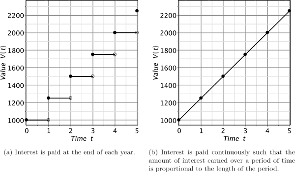
An investment of $1,000 grows by a constant amount of $250 each year for five years. What does the graph of the value function V(t) look like if

1. (a) interest is only paid at the end of each year;
2. (b) interest is paid continuously so that V is a linear function.

Solution. In case (a), the value function is a piecewise step function with jumps at the end of every year, i.e., V (t)= V (t − 1)+250 for all t ≥ 1. In case (b), the value function is a linear function of time t, i.e., V(t)= V (0) + ct for some parameter c. Since V (1) = V (0) + 250, the parameter c is equal to 250, and, therefore, V (t) = 1000 + 250t. The plots of the value functions are given in Figure 1.2.

Typically, the amount your investment is worth at time t is proportional to the principal P you deposited at time 0. Let A(t) denote the accumulated value for principal $1. This function is called the accumulation function. So, one dollar invested at time 0 grows to A(t) at time t. Then the accumulated value for principal P is given by

$V\left(t\right)=P A\left(t\right).\text{ (1.1)}$

Consider an investment with the value function V (t), t ≥ 0. The total return on the investment is the ratio of the amount received at the end of a period to the amount invested at the beginning of the period,

$\text{total} \text{return}=\frac{\text{amount} \text{received}}{\text{amount} \text{invested}}.$

Thus, the total return for the time interval [s, t] with 0 ≤ s < t, denoted R[s,t], on an investment commencing at time s and terminating at time t is

$R_{\left[s,t\right]}=\frac{V\left(t\right)}{V\left(s\right)}.\text{ (1.2)}$

Note that the total return is a function of a period of time rather than a function of an instantaneous time moment.

The rate of return or rate of interest is the ratio of the amount of interest earned during the period to the investment value at the beginning of the period,

$\text{rate} \text{of} \text{return}=\frac{\text{interest} \text{earned}}{\text{amount} \text{invested}}.$

The rate of return for the time interval [s, t], denoted r[s,t], is given by

$r_{\left[s,t\right]}=\frac{V\left(t\right)-V\left(s\right)}{V\left(s\right)}=\frac{V\left(t\right)}{V\left(s\right)}-1.\text{ (1.3)}$

It can be expressed in terms of the accumulation function. For example, for the time interval of t periods from the date of the investment we have

$r_{\left[0,t\right]}=\frac{V\left(t\right)-V\left(0\right)}{V\left(0\right)}=\frac{P A\left(t\right)-P}{P}=A\left(t\right)-1.$

It is clear that the two notions are related by

$R=1+r.$

Equations (1.2) and (1.3) can be rewritten as

$V\left(t\right)=R_{\left[s,t\right]} V\left(s\right)=\left(1+r_{\left[s,t\right]}\right) V\left(s\right).\text{ (1.4)}$

Note that upper-and lowercase letters, such as R and r, are used for total returns and rates of return, respectively. Often, for simplicity, the term return is used for both notions. Let n be a positive integer. The interval [n − 1, n] is the nth year (or the nth period, in general). Denote by Rn and rn the total return and rate of return during the nth year from the date of investment, respectively. That is, we have

$R_n≔R_{\left[n-1,n\right]}=\frac{V\left(n\right)}{V\left(n-1\right)} \text{and} r_n≔r_{\left[n-1,n\right]}=\frac{V\left(n\right)-V\left(n-1\right)}{V\left(n-1\right)}\text{ (1.5)}$

for n = 1, 2, 3,.... The accumulated value V (n) can be now written as follows:

$\begin{array}{ccc}\hfill \frac{V\left(n\right)-V\left(n-1\right)}{V\left(n-1\right)}& =& r\hfill \\ \hfill V\left(n\right)-V\left(n-1\right)& =& rV\left(n-1\right)\hfill \\ \hfill V\left(n\right)& =& \left(1+r\right)V\left(n-1\right),\mathrm{ }\text{with} r=r_n.\hfill \end{array}\text{ (1.6)}$

For two nonnegative integers n and m with n < m, the amount V (m) accumulated by the end of period m can be written in two different ways:

$V\left(m\right)=\left(1+r_{\left[n,m\right]}\right)V\left(n\right)$

and

$\begin{array}{ccc}V\left(m\right)& =& \left(1+r_m\right)V\left(m-1\right)=\left(1+r_{m-1}\right)\left(1+r_m\right)V\left(m-2\right)=...\hfill \\ & =& \left(1+r_{n+1}\right)...\left(1+r_{m-1}\right)\left(1+r_m\right)V\left(n\right).\hfill \end{array}\text{ (1.7)}$

Therefore, one-period returns and aggregate returns are related as follows:

$1+r_{\left[n,m\right]}=\left(1+r_{n+1}\right)\left(1+r_{n+2}\right)...\left(1+r_m\right),\text{ (1.8)}$

$R_{\left[n,m\right]}=R_{n+1} R_{n+2}...R_m.\text{ (1.9)}$

Example 1.2

(The rate of return). Bill invested $200 for 3 years in an account with the accumulation function A(t)=0.1t2 + 1. Find annual returns r1, r2, and r3.

Solution. The accumulated values and returns at the end of years 1, 2, and 3 are, respectively,

$\begin{array}{ccccccccccccccc}V\left(1\right)& =& 200·\left(0.1·1^2+1\right)\hfill & =& 200\hfill & \Rightarrow & r_1\hfill & =& \frac{V\left(1\right)-V\left(0\right)}{V\left(0\right)}\hfill & =& \frac{220-200}{200}\hfill & =& \frac{1}{10}\hfill & =& 10\%,\hfill \\ V\left(2\right)& =& 200·\left(0.1·2^2+1\right)\hfill & =& 280\hfill & \Rightarrow & r_2\hfill & =& \frac{V\left(2\right)-V\left(1\right)}{V\left(1\right)}\hfill & =& \frac{280-220}{220}\hfill & =& \frac{3}{11}\hfill & \cong & 27.27\%,\hfill \\ V\left(3\right)& =& 200·\left(0.1·3^2+1\right)\hfill & =& 380\hfill & \Rightarrow & r_3\hfill & =& \frac{V\left(3\right)-V\left(2\right)}{V\left(2\right)}\hfill & =& \frac{380-280}{280}\hfill & =& \frac{5}{14}\hfill & \cong & 35.71\%.\hfill \end{array}$

Example 1.3

(The accumulated value). Let V (3) = 1000 and $R_n=\frac{3n+2}{2n+2}$, n = 1, 2, 3,.... Find V (6).

Solution. By using (1.4) and (1.9), we obtain

$V\left(6\right)=V\left(3\right)R_4{R}_5{R}_6=1000·\frac{7}{5}·\frac{17}{12}·\frac{10}{7}=\$2,\mathrm{833.33.}$

1.1.2 Simple Interest

For simple interest, the rate of return r[0,t] is proportional to time t measured in years. That is, there exists a positive constant r, called a simple interest rate (per year), so that r[0,t] = r t for all t ≥ 0. In particular, the rate of return for year 1 is r1 = r[0,1] = r. The interest I(t) earned on the original principal P during the time period of length t is then calculated by the simple formula

$I\left(t\right)=r_{\left[0,t\right]}P=rtP.$

The accumulated value after t years will be

$V\left(t\right)=P+I\left(t\right)=P+rtP=\left(1+rt\right)P,\mathrm{ }t\ge 0.\text{ (1.10)}$

Clearly, the accumulated value V (t) is a linear function of time t (see Figure 1.2b).

To find the initial capital (the principal) whose accumulated value at time t is given, we invert the formula (1.10) to obtain

$P=V\left(0\right)=\frac{V\left(t\right)}{1+rt}={\left(1+rt\right)}^{-1}V\left(t\right).\text{ (1.11)}$

This number is called the present or discounted value of the amount V (t), and (1 + rt)−1 is a discount factor at a simple interest rate r. Formula (1.11) allows us to find the original principal P invested at time 0.

Example 1.4.

How long will it take $3,000 to earn $60 interest at 6%?

Solution. We have P = 3000, I = 60, r = 0.06, and then

$t=\frac{I}{Pr}=\frac{60}{3000·0.06}=\frac{1}{3} \text{years}=4 \text{months}\text{.}$

Example 1.5.

Treasury bills (T-bills) are popular short-term securities issued by the Federal Government of Canada with maturities of 1, 3, 6, or 12 months. T-bills are issued in different denominations, or face values. The face value of a T-bill is the amount the government guarantees it will pay on the maturity date. There is no interest stated on a T-bill. Instead, to determine its purchase price, you need to discount the face value to the date of sale at an interest rate that is determined by market conditions.

Suppose that a 6-month T-bill with a face value of $25,000 is purchased by an investor who wishes to yield 3.80%. What price is paid?

Solution. We have V = 25000, $t=\frac{6}{12}$, and r = 0.038. Therefore, the investor will pay

$P=V·{\left(1+rt\right)}^{-1}=25000·{\left(1+0.038·\frac{1}{2}\right)}^{-1}=\$24,533.86$

for the T-bill and receive $25,000 in six months.

Let us study the return on an account earning interest at rate r. The distinction between the interest rate and the rate of return is that the interest rate refers to a period of one year (i.e., interest per annum) and is independent of the actual duration of an investment, whereas the return reflects both the interest rate and the length of time the investment is held. For all 0 ≤ t < s, we have

$r_{\left[t,s\right]}=\frac{V\left(s\right)-V\left(t\right)}{V\left(t\right)}=\frac{\left(1+rs\right)P-\left(1+rt\right)P}{\left(1+rt\right)P}=\frac{\left(s-t\right)r}{1+rt}.$

In particular, for the first year, we have r1 = r[0,1] = r. The rate of return during the nth year from the date of investment is

$r_n=r_{\left[n-1,n\right]}=\frac{r}{1+\left(n-1\right)r}.$

Clearly, these rates form a decreasing sequence that converges to zero as n approaches ∞. In other words, if the investment earns simple interest at the same rate every year, the effective annual rate of return is decreasing. To guarantee constant annual returns, the interest should be reinvested, as is demonstrated in the next section.

1.1.3 Periodic Compound Interest

Assume that the interest earned at a constant rate i > 0 is automatically reinvested, i.e., it will be added to the investment periodically (e.g., annually, semi-annually, quarterly, weekly, daily). In this situation, we are dealing with periodic compounding. The interest is said to be compounded or to be converted.

Example 1.6.

Determine the compound interest earned on $1,000 for 1 year at an annual rate of 8% compounded quarterly and compare it with the simple interest earned on the same amount for 1 year at 8% per annum.

Solution. Since the compounding period is one quarter, the interest rate per period is equal to $\frac{3}{12}\cdot 8\%=2\%$. In the case of simple interest, the amount of interest earned during each quarter is fixed and equal to $1,000 · 0.02 = $20. In the case of compounded interest, the interest earned during one quarter depends on the amount invested at the beginning of the period. The interest on the investment of V dollars is $I=V\cdot 0.08\cdot \frac{1}{4}=V\cdot 0.02$. Results of our calculations are given in Table 1.3.

In summary, the compound interest earned on $1,000 for 1 year at 8% compounded quarterly is $82.43, whereas the simple interest on $1,000 for 1 year at 8% is equal to $1,000 · 0.08 · 1 = $80.

Let δt denote the time between two consecutive interest conversions (this time interval is called an interest conversion period). Assume that there are m interest conversion periods per year, so $\delta t=\frac{1}{m}$. The interest earned during one period is

$I=V i \delta t=V\frac{i}{m},$

where V is the amount invested at the beginning of the period, and i is the annual interest rate. Thus, the interest rate per period of δt is equal to $\frac{i}{m}$. Denote this one-period rate by j. Let us find the accumulated value V (n δt) at the end of period n = 1, 2,.... At the beginning, we have V (0) = P. By compounding the interest at the end of each period, we obtain the following accumulated values:

$\begin{array}{ccc}\text{at the end of the 1st period}\hfill & \hfill \mathrm{ }& V\left(\delta t\right)=V\left(0\right)+jV\left(0\right)=\left(1+j\right)V\left(0\right)=\left(1+j\right)P,\hfill \\ \text{at the end of the 2nd period}\hfill & \hfill \mathrm{ }& V\left(2 \delta t\right)=V\left(\delta t\right)+jV\left(\delta t\right)=\left(1+j\right)V\left(\delta t\right)={\left(1+j\right)}^{2}P,\hfill \\ \text{at the end of the 3rd period}\hfill & \hfill \mathrm{ }& V\left(3 \delta t\right)=\left(1+j\right)V\left(2\delta t\right)={\left(1+j\right)}^{3}P,\hfill \\ & \hfill \mathrm{ }& ⋮\hfill \\ \text{at the end of the} n\text{th period}\hfill & \hfill \mathrm{ }& V\left(n \delta t\right)=\left(1+j\right)V\left(\left(n-1\right)\delta t\right)={\left(1+j\right)}^{n}P.\hfill \end{array}$

Therefore, the accumulated value at time t = n δt is

$V\left(t\right)={\left(1+\frac{i}{m}\right)}^{n}P.\text{ (1.12)}$

The quantity m is called the frequency of compounding. Commonly used frequencies of compounding are m = 1 for annual compounding, m = 2 for semi-annual compounding, m = 4 for quarterly compounding, m = 12 for monthly compounding, m = 52 for weekly compounding, and m = 365 for daily compounding. The length of time between two consecutive interest calculations is called the interest conversion period or just interest period. Let i(m) denote a nominal interest rate that is compounded (convertible) m times per year. Note that i(m) is stated as an annual rate of interest. The interest rate compounded annually is simply denoted by i, i.e., i(1) ≡ i. The interest rate per period of δt = 1/m years is equal to i(m)/m. The accumulated value of $1 at the end of m interest conversion periods (i.e., at the end of one year) is

${\left(1+\frac{i^{\left(m\right)}}{m}\right)}^m.$

Thus, after t years the principal P grows to

$V\left(t\right)={\left(1+\frac{i^{\left(m\right)}}{m}\right)}^{mt}P.\text{ (1.13)}$

Here, mt gives the cumulative number of periods. The factor ${\left(1+\frac{i^{\left(m\right)}}{m}\right)}^m$ is called the accumulation factor over a one-year period, and it is in fact the accumulated value of $1 at the end of one year with m as the compounding frequency. The annual nominal rate is meaningless until we specify the frequency m. At the same nominal rate the accumulated value depends on this frequency; it increases with increasing m. In particular, under interest compounded at the end of every year, the accumulation function is V (t) = (1+ i)tP (see Figure 1.4).

To find the return on a deposit attracting interest periodically compounded, we use the general formula $r_{\left[s,t\right]}=\frac{V\left(t\right)-V\left(s\right)}{V\left(s\right)}$ and readily arrive at:

$r_{\left[s,t\right]}=\frac{V\left(t\right)-V\left(s\right)}{V\left(s\right)}=\frac{V\left(t\right)}{V\left(s\right)}-1={\left(1+\frac{i^{\left(m\right)}}{m}\right)}^{\left(t-s\right)m}-1\mathrm{ }\text{for} 0\le s<t.$

For the nth year the rate of return is

$r_n=r_{\left[n-1,n\right]}={\left(1+\frac{i^{\left(m\right)}}{m}\right)}^m-1.$

As is seen, the annual rate of return rn does not depend on n and is a constant quantity for any given m. It is clear that the return on a deposit subject to periodic compounding is not additive, i.e., $R_{\left[t_1,t_2\right]}+R_{\left[t_2,t_3\right]}\ne R_{\left[t_1,t_3\right]}$ and $r_{\left[t_1,t_2\right]}+r_{\left[t_2,t_3\right]}\ne r_{\left[t_1,t_3\right]}$ for t1 < t2 < t3 in general. For example, take m = 1, then r[0,1] = r[1,2] = r and

$r_{\left[0,2\right]}={\left(1+r\right)}^2-1=2r+r^2\ne 2r=r_{\left[0,1\right]}+r_{\left[1,2\right]}.$

Example 1.7.

Find the total return and rate of return over two years under quarterly compounding with 8% per annum.

Solution. We have

$R_{\left[0,2\right]}={\left(1+\frac{0.08}{4}\right)}^{2.4}={1.02}^8=\mathrm{1.17166.}$

Therefore, r[0,2] = R[0,2] − 1 = 17.166%.

In business transactions it is frequently necessary to determine what principal P now will accumulate at a given interest rate to a specified amount V (t) at a specified future date t. From the fundamental formula (1.13), we obtain

$P=\frac{V\left(t\right)}{{\left(1+i^{\left(m\right)}/m\right)}^{mt}}={\left(1+\frac{i^{\left(m\right)}}{m}\right)}^{-mt}V\left(t\right).\text{ (1.14)}$

P is called the discounted value or present value of V (t). The process of determining P from V (t) is called discounting. Similarly, we can find the value V (s) of an investment at any intermediate date 0 < s < t given the value V (t) at some fixed future time t:

$V\left(s\right)=\frac{V\left(t\right)}{{\left(1+i^{\left(m\right)}/m\right)}^{\left(t-s\right)m}}.$

1.1.4 Continuous Compound Interest

Consider a fixed nominal rate of interest r compounded at different frequencies m. Let us find the limiting value of the accumulated value of $1 over a one-year period as m → ∞ :

${\displaystyle \underset{m\to \infty }{\text{lim}}}{\left(1+\frac{r}{m}\right)}^m={\left({\displaystyle \underset{m\to \infty }{\text{lim}}}{\left(1+\frac{r}{m}\right)}^{\frac{m}{r}}\right)}^r$

(denote r/m by x, which converges to 0 as m → ∞)

$={\left({\displaystyle \underset{x\searrow 0}{\text{lim}}} {\left(1+x\right)}^{\frac{1}{x}}\right)}^r=e^r.$

[Note: The number e = 2.71828 ... is the base of the natural logarithm; it is occasionally called Euler's number.] Therefore, the accumulated value of principal P compounded continuously at rate r over a period of t years (note that t may be fractional) is given by

$V\left(t\right)={\displaystyle \underset{m\to \infty }{\text{lim}}}{\left(1+\frac{r}{m}\right)}^{mt}P={\left[{\displaystyle \underset{m\to \infty }{\text{lim}}}{\left(1+\frac{r}{m}\right)}^m\right]}^{t}P=e^{rt}P.\text{ (1.15)}$

We will denote the continuously compounded interest rate by r rather than by i(∞). The discounted value P for given V (t), r, and t is

$P={\text{e}}^{-rt}V\left(t\right).\text{ (1.16)}$

Being given the annual rate of return $i=\frac{V\left(1\right)-V\left(0\right)}{V\left(0\right)},$ one can find the continuously compounded rate r as follows: r = ln(1 + i).

1.1.5 Equivalent Rates

Two nominal compound interest rates are said to be equivalent if they yield the same accumulated value at the end of one year, and hence at the end of any number of years. For example, the rate i compounded annually and rate i(m) compounded m per year are equivalent iff

$1+i={\left(1+\frac{i^{\left(m\right)}}{m}\right)}^m.$

Example 1.8.

Determine what rate i(4) is equivalent to (a) i(12) = 6%, (b) i(2) = 6%.

Solution.

1. (a) Equate the two accumulation factors, (1 + 0.06/12)12 = (1+ i(4)/4)4, and solve for the rate i(4):

   $i^{\left(4\right)}=4·\left({\left(1+0.06/12\right)}^{12/4}-1\right)=4·\left({\left(1.005\right)}^3-1\right)\cong 6.030\%.$

2. (b) We have (1 + 0.06/2)2 = (1+ i(4)/4)4, hence

   $i^{\left(4\right)}=4·\left({\left(1+0.06/2\right)}^{2/4}-1\right)=4·\left(\sqrt{1.03}-1\right)\cong 5.956\%.$

For a given nominal rate i(m) compounded m times per year or for a rate r compounded continuously, we define the corresponding annual effective rate, i, to be that rate which, if compounded annually, will produce the same interest. In other words, i is the annual rate of interest that is equivalent to i(m) or r. Note that equivalent compound rates have the same annual effective rate. To determine i, we compare the accumulated values of $1 at the end of one year; thus

$i=\{\begin{array}{l}{\left(1+\frac{i^{\left(m\right)}}{m}\right)}^m-1\hfill \\ {\text{e}}^r-1\hfill \end{array}\begin{array}{l}\mathrm{ }\text{for} \text{a} \text{rate} \text{compounded} m \text{times} \text{per} \text{year},\hfill \\ \mathrm{ }\text{for} \text{a} \text{rate} \text{compounded} \text{continuously}\text{.}\hfill \end{array}\text{ (1.17)}$

Example 1.9.

You wish to invest a sum of money for a number of years and have narrowed your choices to the following three investments:

1. A at the interest rate i(2) = 10.35%;
2. B at the interest rate i(12) = 10.15%;
3. C at the interest rate i(4) = 10.25%.

Which investment should you choose?

Solution. To decide which investment is best, you need to calculate the equivalent rate compounded with the same frequency (e.g., annually) for each investment. So, let us calculate the annual effective rate of interest for each investment:

1. A: $i={\left(1+\frac{0.1035}{2}\right)}^2-1\cong 10.6178\%;$
2. B: $i={\left(1+\frac{0.1015}{12}\right)}^{12}-1\cong 10.6358\%;$
3. C: $i={\left(1+\frac{0.1025}{4}\right)}^4-1\cong 10.6508\%.$

It turns out that investment C has the highest annual effective rate, so you should choose this investment.

Example 1.10.

Determine rates i(2) and i(12) that are equivalent to r = 6%.

Solution. We equate the annual accumulation factors at each interest rate to obtain

$\begin{array}{llll}\hfill {\left(1+i^{\left(2\right)}/2\right)}^2& ={\text{e}}^{0.06}\hfill & \hfill {\left(1+i^{\left(12\right)}/12\right)}^{12}& ={\text{e}}^{0.06}\hfill \\ \hfill i^{\left(2\right)}/2& ={\text{e}}^{0.06/2}-1\hfill & \hfill i^{\left(12\right)}/12& ={\text{e}}^{0.06/12}-1\hfill \\ \hfill i^{\left(2\right)}& \cong 6.091\%\hfill & \hfill i^{\left(12\right)}& \cong 6.015\%\hfill \end{array}$

We can generalize the result presented above and state that for rates of interest that are all equivalent we have

$i^{\left(1\right)}>i^{\left(2\right)}>i^{\left(4\right)}>i^{\left(12\right)}>i^{\left(365\right)}>i^{(\infty )},\text{ (1.18)}$

where i(1) ≡ i and i(∞) ≡ r.

Proposition 1.1.

For a fixed annual effective rate i, the compound interest rates i(m), where m = 1, 2, 3,..., all equivalent to i, form a decreasing sequence that converges to the rate r = ln(1 + i) as m → ∞.

Proof. The interest rate i(m) is equivalent to the annual effective rate i iff (1+ i(m)/m)m = 1 + i holds. This defines the interest rate i(m) ≡ i(m) as a function of m > 0:

$i\left(m\right)=\left({\left(1+i\right)}^{1/m}-1\right)m=\left(e^{r/m}-1\right)m.$

Hence, its derivative w.r.t. m is

$i\text{'}\left(m\right)=i\left(m\right)/m-\left(r/m\right){\text{e}}^{r/m}=i\left(m\right)/m-\left(1+i\left(m\right)/m\right)ln\left(1+i\left(m\right)/m\right).$

Let us prove that the derivative i'(m) is strictly negative for all m > 0.

• To show that (1 + i(m)/m) ln(1 + i(m)/m) > i(m)/m holds for all m > 0, it suffices to prove that the inequality ln(1 + x) > x/(1 + x) holds for all x > 0.
• Notice that if two functions f(x) and g(x) are such that f(0) ≥ g(0) and f'(x) >g'(x) holds for all x > 0, then f(x) > g(x) is valid for all x > 0.
• Let f(x) ≔ ln(1 + x) and g(x) ≔ x/(1 + x)=1 − (1 + x)−1 . Their derivatives are f'(x) = (1+ x)−1 and g'(x) = (1+ x)−2, respectively.
• Clearly, (1 + x)−1 > (1 + x)−2 holds for all x > 0. Since f(0) = g(0) = 0, we obtain that ln(1 + x) > x/(1 + x) is valid for all x > 0.

Using l'Hôpital's rule (LHR) gives

${\displaystyle \underset{m\to \infty }{\text{lim}}}{i}^{\left(m\right)}={\displaystyle \underset{m\to \infty }{\text{lim}}}\frac{{\text{e}}^{r/m}-1}{1/m}={\displaystyle \underset{t\to 0}{\text{lim}}}\frac{{\text{e}}^{rt}-1}{t}\stackrel{\left(\text{LHR}\right)}{=}{\displaystyle \underset{t\to 0}{\text{lim}}} r{\text{e}}^{rt}=r {\displaystyle \underset{t\to 0}{\text{lim}}} e^{rt}=r.$

Proposition 1.2.

The accumulation function $A(m)={\left(1+\frac{r}{m}\right)}^m$ for a fixed nominal interest rate r compounded with frequency m over a one-year period is a strictly increasing function of m that converges to er as m →∞.

Proof. Differentiate the function A(m) w.r.t. m to obtain

$A\text{'}\left(m\right)={\left(1+r/m\right)}^m\left(ln\left(1+r/m\right)-\frac{r/m}{1+r/m}\right).$

Using the inequality ln(1 + x) > x/(1 + x) with x = r/m > 0 gives that A'(m) > 0. Therefore, {A(m)}m≥1 is a strictly increasing sequence that converges to er as m →∞.

As follows from the above proposition, continuous compounding produces higher accumulated value than periodic compounding with any frequency m, that is, ${\left(1+\frac{r}{m}\right)}^m<{\text{e}}^r$ for all m ≥ 1.

Example 1.11.

Consider an investment at: (a) simple interest rate 6%, (b) annual compound interest rate 6%, and (c) continuous compound interest rate 6%. Find the time that is necessary to double the original principal.

Solution. For each investment, we find time t so that the respective accumulation function equals 2.

1. (a) For simple interest: 1 + 0.06t = 2, hence t = 1/0.06 ≅ = 16.67 years.
2. (b) For interest compounded annually: (1 + 0.06)t = 2, hence $t=\frac{ln2}{ln1.06}\cong 11.9$ years.
3. (c) For interest compounded continuously: e0.06t = 2, hence $t=\frac{ln2}{0.06}\cong 11.55$ years.

Let us summarize the above three methods of calculating interest. The accumulation function $A(t)=\frac{V\left(t\right)}{V\left(0\right)}=R_{\left[0,t\right]}$ has the following form:

$A\left(t\right)=\{\begin{array}{ll}1+rt\hfill & \text{for} \text{a} \text{rate} \text{of} \text{simple} \text{interest},\hfill \\ {\left(1+\frac{i^{\left(m\right)}}{m}\right)}^{mt}\hfill & \text{for} \text{a} \text{rate} \text{of} \text{interest} \text{compounded} \text{periodically},\hfill \\ {\text{e}}^{rt}\hfill & \text{for} \text{a} \text{rate} \text{of} \text{interest} \text{compounded} \text{continuously}.\hfill \end{array}\text{ (1.19)}$

In what follows, we will also use the discounting function $D(t)=\frac{V\left(0\right)}{V\left(t\right)}=\frac{1}{A\left(t\right)}$ taking the form:

$D\left(t\right)=\{\begin{array}{ll}{\left(1+rt\right)}^{-1}\hfill & \text{for} \text{a} \text{rate} \text{of} \text{simple} \text{interest},\hfill \\ {\left(1+\frac{i^{\left(m\right)}}{m}\right)}^{-mt}\hfill & \text{for} \text{a} \text{rate} \text{of} \text{interest} \text{compounded} \text{periodically},\hfill \\ {\text{e}}^{-rt}\hfill & \text{for} \text{a} \text{rate} \text{of} \text{interest} \text{compounded} \text{continuously}.\hfill \end{array}\text{ (1.20)}$

1.1.6 Continuously Varying Interest Rates

Consider the case of continuously compounded interest but with a rate that is changing in time. Let T be the time horizon of investment; let r(t) denote the instantaneous interest rate at time t ∊ [0,T]. Consider a time interval [t, t + δt] with small δt > 0. Suppose that the rate r(t) is approximately constant on the interval [t, t + δt]. Then the amount V (t) invested at time t will grow to V (t + δt)= V (t)er(t) δt at time t + δt.

Let the principal P be invested at time 0. To determine V (t) in terms of the principal and the instantaneous interest rate function r(t) for 0 ≤ t ≤ T, we split the time interval [0,T] in N equal subintervals of length δt = T/N and apply the above approach. For times tk = k δt with k = 0, 1,...,N, we obtain

$\begin{array}{ccc}V\left(t_1\right)& \hfill =\hfill & V\left(t_0\right)e^{r\left(t_0\right)\delta t}=P{\text{e}}^{r\left(t_0\right)\delta t}\hfill \\ V\left(t_2\right)& \hfill =\hfill & V\left(t_1\right)e^{r\left(t_1\right)\delta t}=P{\text{e}}^{\left(r\left(t_0\right)+r\left(t_1\right)\right)\delta t}\hfill \\ V\left(t_3\right)& \hfill =\hfill & V\left(t_2\right)e^{r\left(t_2\right)\delta t}=P{\text{e}}^{\left(r\left(t_0\right)+r\left(t_1\right)+r\left(t_2\right)\right)\delta t}\hfill \\ & \hfill ⋮\hfill \\ V\left(t_N\right)& \hfill =\hfill & P{\text{e}}^{\left(r\left(t_0\right)+r\left(t_1\right)+...+r\left(t_{N-1}\right)\right)\delta t}=Pexp\left({\displaystyle \sum _{k=0}^{N-1}}r\left(t_k\right)\delta t\right).\hfill \end{array}$

Recognizing the Riemann sum in the last equation with the time step δt = T/N and taking the limit as N → ∞, we have

${ }_{N\to \infty }^{lim}{\displaystyle \sum _{k=0}^N}r\left(t_k\right)\delta t={\displaystyle {\int }_0^T}r\left(t\right)\text{d}t.$

Therefore, the value at the maturity time T is given by

$V\left(T\right)=Pexp\left({\displaystyle {\int }_0^T}r\left(t\right)\text{d}t\right).\text{ (1.21)}$

If r(t) is constant and equal to r for all t ∊ [0,T], then (1.21) reduces to the usual formula for the accumulated value under continuous compounding:

$V\left(T\right)=Pexp\left({\displaystyle {\int }_0^T}r\text{d}t\right)=Pexp\left(r{\displaystyle {\int }_0^T}\text{d}t\right)=Pexp\left(rT\right).$

Let y(T) denote the average of the instantaneous interest rates from time 0 to time T:

$y\left(T\right)≔\frac{1}{T}{\displaystyle {\int }_0^T}r\left(t\right)\text{d}t.$

Then, (1.21) takes a familiar form:

$V\left(T\right)=P{\text{e}}^{y\left(T\right)T}.$

The interest rate y(T) is called the yield rate or spot rate for maturity T.

It is possible to derive (1.21) in a different way. Consider an investment with principal V (0) = P and accumulated value V (t) at time t > 0. The nominal rate of interest compounded m times per year and evaluated at time t is given by

$i^{\left(m\right)}\left(t\right)=\frac{V\left(t+\frac{1}{m}\right)-V\left(t\right)}{\frac{1}{m}V\left(t\right)}.$

Let $\delta t=\frac{1}{m}$, so that, as m → ∞ and δt → 0, we have

$r\left(t\right)≔{ }_{m\to \infty }^{lim} i^{\left(m\right)}\left(t\right)={ }_{\delta t\to 0}^{lim}\frac{V\left(t+\delta t\right)-V\left(t\right)}{\delta tV\left(t\right)}=\frac{V\text{'}\left(t\right)}{V\left(t\right)}=\frac{dlnV\left(t\right)}{\text{d}t}.\text{ (1.22)}$

Thus, r(t) is a measure of the relative instantaneous rate of growth at time t. It is sometimes called the force of interest. Integrating $r\left(t\right)=\frac{d\ln V\left(t\right)}{d\text{t}}$ from 0 to T gives

${\displaystyle {\int }_0^T}r\left(t\right)\text{d}t={\displaystyle {\int }_0^T}\frac{dlnV\left(t\right)}{\text{d}t} \text{d}t=lnV\left(T\right)-lnV\left(0\right)=ln\left(\frac{V\left(T\right)}{V\left(0\right)}\right),$

and then (1.21) follows by exponentiation.

Example 1.12.

Calculate the accumulated value of $1,000 at the end of 4 years if r(t)= 0.05 + 0.1t.

Solution. The accumulation function is

$A\left(T\right)=exp\left({\displaystyle {\int }_0^T}r\left(d\right)\text{d}t\right)=exp\left({\displaystyle {\int }_0^T}\left(0.05+0.1t\right)\text{d}t\right)={\text{e}}^{0.05T+0.05T^2}$

for every T ≥ 0. Thus, after 4 years we have

$A\left(4\right)={\text{e}}^{0.05·4+0.05·4^2}=\text{e}\cong 2.71828182$

and V (4) = P A(4) = 1000e ≅ = $2,718.28.

1.2 Time Value of Money and Cash Flows

1.2.1 Equations of Value

All financial decisions must take into account the basic idea that money has its time value. In order to compare or add different amounts of money we must place the amounts at the same point in time, called the focal date. The mathematics of finance deals with dated values. In general, we compare dated values by the following definition of equivalence.

Definition 1.1.

Assume the periodic compounding of interest. Amount $X due on a given date is equivalent to $Y due n interest conversion periods later, if Y = X(1 + j)n or X = Y (1 + j)−n, where j = i(m)/m and i(m) is a given compound interest rate. The following time diagram illustrates dated values equivalent to a given dated value X.

We say that two sets of payments are equivalent at a given interest rate if the dated values of the sets, on any common date, are equal. An equation stating that the dated values of two sets of payments are equal is called an equation of value.

Example 1.13.

A debt of $5,000 is due at the end of 3 years. Determine an equivalent debt due at the end of (a) 3 months, (b) 3 years and 9 months. Assume quarterly compounding with i(4) = 12%.

Solution. We arrange the data on a time diagram below where one period is 3 months.

By the definition of equivalence:

1. (a) X1 = $5,000 · (1 + 0.12/4)−11 = $5,000 · (1.03)−11 ≅ = $3,612.11;
2. (b) X2 = $5,000 · (1 + 0.12/4)3 = $5,000 · (1.03)3 ≅ $5,463.64.

Example 1.14.

A debt of $5,000 is due at the end of 5 years. It is proposed that $X be paid now and with another $X paid in 10 years' time to liquidate the debt. Calculate the value of X if the effective interest rate is 12% for the first 6 years and 8% for the next 4 years.

Solution. The value of the first payment at time t = 5 is X · (1.12)5 . The value of the second payment at time t = 5 is X · (1.08)−4 · (1.12)−1 . We equate the sum of these two values and the value of the debt of $5,000 at t = 5 to obtain

$5000=X·{\left(1.12\right)}^5+X·{\left(1.08\right)}^{-1}·{\left(1.12\right)}^{-1}=X·\left(1.76234+0.656277\right)=2.41862 X.$

Hence, X = $5,000/2.41862 ≅ = $2,067.30.

Example 1.15.

Suppose you can buy a house for $84,000 cash (option 1) or for payments of $50,000 now, $20,000 in 1 year, and $20,000 in 2 years (option 2). If money is worth i(12) = 9%, which option is more profitable?

Solution. The discounted value of option 1 is $84,000. Using monthly compounding, the discounted value of option 2 is

$\begin{array}{l}\$50,000+\$20,000·{\left(1+0.09/12\right)}^{-12}+\$20,000·{\left(1+0.09/12\right)}^{-24}\hfill \\ \cong \$50,000+\$18,248.76+\$16,716.63=\$85,001,39.\hfill \end{array}$

Clearly, option 1 is more preferable than option 2.

Example 1.16.

If you file your taxes late, the Canada Revenue Agency charges you an immediate 5% late penalty, as well as 5% compounded daily on your outstanding balance. Express my total penalty as a single rate (compounded daily) assuming I pay 26 weeks late.

Solution. If I pay n days late, every dollar I originally owed swells to

$1.05·{\left(1+0.05/365\right)}^n.$

Therefore, on a per dollar basis my total debt after n = 26 · 7 = 182 days is

$1.05·{\left(1+0.05/365\right)}^{182}.$

Had I been charged the single rate i(365), my total debt would have been (1 + i(365)/365)182 . Equating and solving for i(365) we get

$1.05·{\left(1+0.05/365\right)}^{182}={\left(1+i^{\left(365\right)}/365\right)}^{182},$

which can be rearranged to find

$i^{\left(365\right)}=365·\left({1.05}^{1/182}·\left(1+0.05/365\right)-1\right)\cong \mathrm{0.14787.}$

Therefore my effective penalty rate is approximately 14.79%.

Remark. If I pay n days late, then my penalty rate is

$i_n^{\left(365\right)}=365·\left({1.05}^{1/n}\left(1+0.05/365\right)-1\right).$

Observe that ${\lim }_{n\to \infty }{i}_n^{\left(365\right)}=0.05$. Thus, if I pay extremely late, the initial 5% penalty is dwarfed by the compound interest. Of course, this does not mean that it is a good idea to pay extremely late.

Remark. Suppose you are offered a Guaranteed Investment Certificate (GIC) that promises 4% compounded annually with an upfront service fee of 1% of the amount invested. If invested for n years, the effective rate that you earn on the GIC can be determined by solving $0.99·{\left(1+r\right)}^n={\left(1+i^{\left(n\right)}\right)}^n$, which yields i(n) = 0.991/n · (1 + r) − 1. It is easy to prove (do this as an exercise) that i(n) is less than r and converges to r as n → ∞.

Example 1.17.

You have access to an account that pays 100r% per annum, compounded annually. You are given two options to repay a debt. Option A is an immediate payment of $30,000; option B is the payment of $16,000 per year for each of the next two years. For what values of r would you choose option B?

Solution. The present value of B, in thousands of dollars, is

$P_B\left(r\right)=\frac{16}{1+r}+\frac{16}{{\left(1+r\right)}^2}.$

The present value of A, in thousands of dollars, is PA(r) = 30. It is only sensible to choose option B provided PB(r) <PA(r), which occurs if and only if

$30>\frac{16}{1+r}+\frac{16}{{\left(1+r\right)}^2}\iff 30{\left(1+r\right)}^2>16\left(1+r\right)+16,$

which clearly occurs if and only if 30r2 + 44r − 2 > 0. The roots of this quadratic are r ≅ −1.510 and r ≅ 0.0441, and since the leading coefficient of the quadratic is positive we should therefore choose option B if r exceeds the larger root. In summary, we choose A if the interest rate is less than (approximately) 4.41% and choose B otherwise.

1.2.2 Deterministic Cash Flows

From a broad point of view, an investment can be defined as a sequence of expenditures and receipts spanning a period of time. Let all expenses and incomes be denominated in cash. The series of cash payments over a period of time is called a cash flow stream. Suppose that the total time interval [0,T] is divided into n subintervals. Let the payments of C0,C1,...,Cn dollars be respectively received on the dates t0,t1,...,tn so that 0 = t0 < t1 <t2 < ... < tn = T. Table 1.6 represents such a scenario.

A cash flow stream can also be represented as a pair (C, T) of two vectors:

$\text{C}=\left[C_0,C_1,...,C_n\right]\mathrm{ }\text{and}\mathrm{ }\text{T}=\left[t_0,t_1,...,t_n\right].$

Every coin has two sides. If one party holds the cash flow stream C, then the opposite party holds the stream −C =[−C0, −C1,..., −Cn]. Here, we assume that if Ck > 0, then the payment of Ck dollars is received at time tk (an in-flow of cash); if Ck < 0, then the payment of |Ck| dollars is made to the counter-party at time tk (an out-flow of cash).

To visualize a cash flow stream (C, T), one can also use a time diagram which is constructed as follows. First, draw a horizontal line, which represents time increasing from the present (denoted by 0) as we are moving from left to right. After that, draw short vertical lines that start on the horizontal line. Those that go up represent cash coming in (positive cash flows, or receipts), while those that go down represent cash going out (negative cash flows, or disbursements). In general, without knowing the sign of Ck we cannot, on the time diagram, correctly indicate whether Ck should be above or below the time line. The cash flow stream for compounding is given in in Figure 1.7.

Here, the time is measured in periods; j = i(m)/m is the interest rate for one period. This rate is assumed to be constant. The cash flow stream for discounting is represented in Figure 1.8.

Definition 1.2.

The net present value, NPV, of an investment is the difference between the present value of the cash inflows (Ck > 0) and the present value of the cash outflows (Ck < 0), that is,

$\text{NPV}\left(\text{C}\right)=C_0+D\left(t_1\right)C_1+D\left(t_2\right)C_2+...+D\left(t_n\right)C_n,\text{ (1.23)}$

where d is the discounting function given by (1.20).

For example, let us assume that the lengths of the periods (tk−1,tk), k = 1, 2,...,n, are equal, and interest is periodically compounded at interest rate j. Then

$\text{NPV}\left(\text{C}\right)=C_0+C_1{\left(1+j\right)}^{-1}+C_2{\left(1+j\right)}^{-2}+...+C_n{\left(1+j\right)}^{-n}.$

The interest rate used is known as the cost of capital and can be considered as the cost of borrowing money by the business or the rate of return that an investor may obtain if the money is invested with security. The NPV can be used to make a business decision. If NPV ≥ 0, we can conclude that the rate of return from the cash in-flows is greater than or equal to the cost of the cash out-flows and the project has economic merit and should proceed. If NPV < 0, the project should not proceed. When attempting to choose between two investments with the same levels of risk, the investor generally chooses the one with the higher net present value. If both investments have the same net present value and the same time interval, then the investor is said to be indifferent between the investments.

Example 1.18

(Calculating the NPV). An investor is considering two investments with the following annual cash flows:

Which is the better investment if the prevailing annual compound interest rate is (a) i = 4.5%; (b) i = 9%?

Solution.

(a) At 4.5%, we have

$\begin{array}{lll}\text{NPV}\text{of}\text{Investment}1\hfill & =\hfill & -13000+\frac{5000}{1+0.045}+\frac{6000}{{\left(1+0.045\right)}^2}+\frac{7000}{{\left(1+0.045\right)}^3}\hfill \\ \hfill & =\hfill & \$3,413.14,\hfill \\ \text{NPV}\text{of}\text{Investment}2\hfill & =\hfill & -13000+\frac{7000}{1+0.045}+\frac{4800}{{\left(1+0.045\right)}^2}+\frac{6000}{{\left(1+0.045\right)}^3}\hfill \\ \hfill & =\hfill & \$3,\mathrm{351.85.}\hfill \end{array}$

Thus, at i = 4.5%, Investment 1 is a better choice.

(b) At 9%, we have

$\begin{array}{lll}\text{NPV}\text{of}\text{Investment}1\hfill & =\hfill & -13000+\frac{5000}{1+0.09}+\frac{6000}{{\left(1+0.09\right)}^2}+\frac{7000}{{\left(1+0.09\right)}^3}\hfill \\ \hfill & =\hfill & \$2,042.52,\hfill \\ \text{NPV}\text{of}\text{Investment}2\hfill & =\hfill & -13000+\frac{7000}{1+0.09}+\frac{4800}{{\left(1+0.09\right)}^2}+\frac{6000}{{\left(1+0.09\right)}^3}\hfill \\ \hfill & =\hfill & \$2,\mathrm{095.18.}\hfill \end{array}$

Thus, at i = 9%, Investment 2 is a better choice.

1.3 Annuities

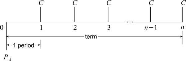
One of the main types of a cash flow stream is an annuity, which is defined as a sequence of periodic payments, usually equal, made at equal intervals of time. There are many examples of annuities in the financial world: mortgage payments on a home, car loan payments, payments on rent, dividends, payments on instalment purchases, etc. The following standard terminology is used.

• The time between successive payments of an annuity is called the payment interval.
• The time from the beginning of the first payment interval to the end of the last payment interval is called the term of an annuity.
• The payments of an ordinary annuity (also known as an annuity immediate) are made at the end of the payment intervals. When the payments are made at the beginning of the payment intervals, the annuity is called an annuity due.
• When the payment interval and interest conversion period coincide, the annuity is called a simple annuity, otherwise it is a general annuity.

We define the accumulated value of an annuity as the equivalent dated value of the set of payments due at the end of the term. Similarly, the discounted value of an annuity is defined as the equivalent dated value of the set of payments due at the beginning of the term. Throughout this section, we shall use the following notations.

1.3.1 Simple Annuities

1.3.1.1 Ordinary Annuities

The present value PA of an ordinary simple annuity is defined as the equivalent dated value of the set of payments due at the beginning of the term, i.e., one period before the first payment. The accumulated value VA of an ordinary simple annuity is defined as the equivalent dated value of the set of payments due at the end of the term, i.e., on the date of the last payment. In Figure 1.9 we display an ordinary simple annuity on a time diagram. The cash flow streams for the repayment of a loan amounting to PA and for the accumulation of a fund amounting to VA are given in Tables 1.10 and 1.11, respectively.

Now we develop a formula for the accumulated value VA of an ordinary simple annuity of n payments of $C using the sum of a geometric progression. Let V (k) denote the accumulated value at the end of period k. At the end of 3 periods, we have

At the end of n periods, we obtain

$V_A=V\left(n\right)=C+\left(1+j\right)C+{\left(1+j\right)}^{2}C+{\left(1+j\right)}^{3}C+...+{\left(1+j\right)}^{n-1}C.\text{ (1.24)}$

Recall the formula for the sum of a geometric progression. For real and positive a and q ≠ = 1, and natural m, we have

$a+aq+a{q}^2+...+a{q}^m=a\sum _{k=0}^m{q}^k=a\frac{q^{m+1}-1}{q-1}.$

Applying this formula to a geometric progression in (1.24) with m = n − 1 terms, whose first term is a = C and common ratio is q = 1 + j, we obtain the accumulated value VA of an ordinary simple annuity of n payments of $C each:

$V_A=C\frac{{\left(1+j\right)}^n-1}{j}.\text{ (1.25)}$

To calculate the periodic payment we solve equation (1.25) for C to obtain

$C=V_A\frac{j}{{\left(1+j\right)}^n-1}.$

It is possible to derive the discounted value PA in several different ways. First, let us consider the amortization of a loan by regular payments of $C. At the end of 2 periods, we have

At the end of n periods, we obtain

$V\left(n\right)={\left(1+j\right)}^n{P}_A\underset{=-V_A}{\underbrace{-C-{\left(1+j\right)}^{1}C-{\left(1+j\right)}^{2}C-...-{\left(1+j\right)}^{n-1}C}}={\left(1+j\right)}^n{P}_A-V_A=0.$

Therefore,

$V_A={\left(1+j\right)}^n{P}_A.\text{ (1.26)}$

Note that this relation also follows directly from the fact that PA and VA are both dated values of the same set of payments and thus they are equivalent. Therefore, the basic formula for the discounted value PA of an ordinary simple annuity of n payments of $C each is

$\begin{array}{lll}{P}_A\hfill & =\hfill & {\left(1+j\right)}^{-n}{V}_A=C{\left(1+j\right)}^{-n}\frac{{\left(1+j\right)}^n-1}{j}=C\frac{1-{\left(1+j\right)}^{-n}}{j}\hfill \\ \hfill & =\hfill & C\frac{1-{\left(1+j\right)}^{-n}}{j}.\hfill \end{array}\text{ (1.27)}$

It is convenient to use the following standard notation:

${\alpha }_{\overline{n|}}=\frac{1-{\left(1+j\right)}^{-n}}{j}.$

This number is called an annuity symbol (read “a angle n at j”). It is the present value of an ordinary simple annuity of n payments of $1 each. The expressions for PA and VA take the following concise forms:

$P_A=C{a}_{\overline{n|}j,}\mathrm{ }{V}_A=C{a}_{\overline{n|}j}{\left(1+j\right)}^n.\text{ (1.28)}$

The formulae (1.25) and (1.27) can also be derived by using the fact that the NPV of the respective cash flow stream is zero:

$\begin{array}{l}\text{NPV}\left(P_A,\underset{n \text{payments}}{\underbrace{-C,...,-C}}\right)=P_A-C_D\left(1\right)-CD\left(2\right)-...-CD\left(n\right)=0\hfill \\ \mathrm{ }\mathrm{ }\Rightarrow P_A=C\sum _{k=1}^n{\left(1+j\right)}^{-k}=C\frac{1-{\left(1+j\right)}^{-n}}{j}\hfill \\ \text{NPV}\left(0,\underset{n \text{payments}}{\underbrace{-C,...,-C}}+V_A\right)=-CD\left(1\right)-CD\left(2\right)-...-CD\left(n\right)+V_{A}D\left(n\right)=0\hfill \\ \mathrm{ }\mathrm{ }\Rightarrow V_A=\frac{C}{D\left(n\right)}\sum _{k=1}^n{\left(1+j\right)}^{-k}=C{\left(1+j\right)}^n\frac{1-{\left(1+j\right)}^{-n}}{j}=C\frac{{\left(1+j\right)}^n-1}{j}.\hfill \end{array}$

Here, D(k) = (1 + j)−k is the discounting function.

Example 1.19.

You make deposits of $1,500 every six months starting today into a fund that pays interest at i(2) = 7%. How much do you have in your fund immediately after the 30th deposit?

Solution. We have C = 1500, n = 30, and the interest rate 0.07/2=0.035 per half year. Since we have been asked to determine the accumulated value on the date of the 30th deposit, we deal with an ordinary simple annuity. Therefore,

$V_A=1500·\frac{{\left(1.035\right)}^{30}-1}{0.035}\cong \$77,\mathrm{434.02.}$

Example 1.20.

It is estimated that a machine will need replacing 10 years from now at a cost of $80,000. How much must be put aside each year to provide that amount of money if the company's savings earn interest at an 8% annual effective rate?

Solution. Assume that an amount of $C is deposited at the end of each of 10 years. So we deal with an ordinary simple annuity. The accumulated value is

$V_A=C\frac{{\left(1.08\right)}^{10}-1}{0.08}=\$80,000.$

Hence, C ≅ = $5,522.36.

Example 1.21.

A used car is purchased for $2,000 down and $200 a month for 6 years. Interest is at i(12) = 10%.

1. (a) Determine the price of the car.
2. (b) Assuming no payments are missed, what single payment at the end of 2 years will completely pay off the debt?

Solution.

(a) We have that the price P of the car is a sum of the down payment and the present value PA of a simple annuity paying $200 a month:

$P=2000+P_A=2000+200\frac{1-{\left(1.008333\right)}^{-72}}{0.008333}\cong \$12,\mathrm{795.73.}$

(b) The value of the debt at the end of 2 years is given by the sum of one regular monthly payment and the present value of 48 = 4 · 12 payments left:

$200+200\frac{1-{\left(1.008333\right)}^{-48}}{0.008333}\cong \$8,\mathrm{085.63.}$

1.3.1.2 Annuities Due

An annuity due is an annuity whose periodic payments are due at the beginning of each payment interval. The term of an annuity due starts at the time of the first payment and ends one payment period after the date of the last payment. The diagram below shows the simple case of an annuity due for n payments when the payment intervals and interest periods coincide.

Annuities due (and deferred annuities presented below) may be handled using the concept of an equation of values. The accumulated value of the payments on the date of the last nth payment (which is time n − 1) is $C a_{\overline{n|}j}{\left(1+j\right)}^n$. We then accumulate this amount for one interest period to obtain the accumulated value VA of an annuity due:

$V_A=C{a}_{\overline{n|}j}{\left(1+j\right)}^{n+1}.\text{ (1.29)}$

The discounted value of the payments one interest period before the first payment is $C{a}_{\overline{n|}j}$. We then accumulate this amount for one interest period to determine the present value PA of an annuity due:

$P_A=C{a}_{\overline{n|}j}\left(1+j\right).\text{ (1.30)}$

Example 1.22.

Determine the discounted value and the accumulated value of $400 payable semi-annually at the beginning of each half-year over 10 years if interest is 8% per year payable semi-annually.

Solution. We deal with an annuity due. There are n = 20 payment periods. The interest rate over one period of 6 months is 0.08/2=0.04. Therefore,

$\begin{array}{c}{V}_A=400\frac{{1.04}^{20}-1}{0.04}\left(1+0.04\right)=400·30.9692\cong \$12,387.68,\\ P_A=400\frac{1-{1.04}^{-20}}{0.04}\left(1+0.04\right)=400·14.1339\cong \$5,\mathrm{653.58.}\end{array}$

1.3.1.3 Deferred Annuities

A deferred annuity is an annuity whose first payment is due some time later than the end of the first interest period. Thus, an ordinary deferred annuity is an ordinary simple annuity whose term is deferred for, say, k periods. The time diagram below depicts this case.

Deferred annuities may be handled using the concept of an equation of values. The period of deferment is k periods and the first payment of the ordinary annuity is at time k + 1. This is because the term of an ordinary annuity starts one period before its first payment. Hence, the discounted value one period before the first payment (time k) is $C a_{\overline{n|}j}$; the discount factor for k periods is (1+j)−k. Therefore, the present value PA of an ordinary deferred annuity is given by

$P_A=C{ }_{a\overline{n|}j}{\left(1+j\right)}^{-k}.\text{ (1.31)}$

Example 1.23.

A used car sells for $9,550. Brent wishes to pay for it in 18 monthly instalments, the first due in three months from the day of purchase. If 12% compounded monthly is charged, determine the size of the monthly payment.

Solution. The discounted value of the deferred annuity is

$9550=C\frac{1-{1.01}^{-18}}{0.01}{1.01}^{-2}=C·\mathrm{11.033308.}$

Hence, the monthly payment is $C=\frac{9550}{11.033308}\cong \$865.56$.

1.3.2 Determining the Term of an Annuity

In some problems, the accumulated value VA or the discounted value PA, the periodic payment C, and the rate j are specified. This leaves the number of payments n to be determined. Note that n can be found by using logarithms:

$\begin{array}{lll}{V}_A\hfill & =\hfill & C\frac{{\left(1+j\right)}^n-1}{j}\Rightarrow {\left(1+j\right)}^n=\frac{j{V}_A}{C}+1\Rightarrow n=\frac{\ln \left(j{V}_A/C+1\right)}{\ln \left(1+j\right)}\hfill \\ P_A\hfill & =\hfill & C\frac{1-{\left(1+j\right)}^{-n}}{j}\Rightarrow {\left(1+j\right)}^{-n}=1-\frac{j{P}_A}{C}\Rightarrow n=-\frac{\ln \left(1-j{P}_A/C\right)}{\ln \left(1+j\right)}.\hfill \end{array}$

Usually, being given VA or PA, C, and j, we cannot find an integer number of periods n for the annuity. It is necessary to make the concluding payment differ from C in order to have equivalence. There are two ways, as follows.

Procedure 1.

The last payment is increased by a sum that will make the payments equivalent to the accumulated value VA or the discounted value PA. This increase is sometimes referred to as a balloon payment.

Procedure 2.

A smaller concluding payment is made one period after the last full payment. The smaller concluding payment is sometimes referred to as a drop payment.

Example 1.24.

A debt of $4,000 bears interest at i(2) = 8%. It is to be repaid by semi-annual payments of $400. Determine the number of full payments needed. Use both Procedure 1 and Procedure 2.

Solution. We have PA = 4000, C = 400, i(2)/2 = 0.08/2=0.04, and we want to calculate n. Substituting in equation (1.27), we obtain:

$\frac{1-{\left(1+0.04\right)}^{-n}}{0.04}=10\Rightarrow -nln\left(1.04\right)=ln\left(0.6\right)\Rightarrow n=\mathrm{13.024.}$

Procedure 1.

There will be 12 regular payments and a final payment. Let X be the balloon payment that will be added to the last regular payment to make the payments equivalent to the discounted value PA = 4000. Using time 0 as the focal date, we obtain the following equation of value:

$\begin{array}{l}400\frac{1-{\left(1+0.04\right)}^{-13}}{0.04}+X{\left(1+0.04\right)}^{-13}=4000\hfill \\ \mathrm{ }\Rightarrow X={1.04}^{13}·\left(4000-400\frac{1-{1.04}^{-13}}{0.04}\right)\hfill \\ \mathrm{ }\Rightarrow X=5.7409·{1.04}^{13}\cong \$\mathrm{9.56.}\hfill \end{array}$

So the last, 13th payment, will be 400 + 9.56 = $409.56.

Procedure 2.

There will be 13 full payments and a final smaller payment. Let Y be the size of a smaller concluding payment (the drop payment). Using time 0 as the focal date, we obtain the following equation of value:

$400\frac{1-{1.04}^{-13}}{0.04}+Y {1.04}^{-14}=4000\Rightarrow Y=5.7409·{1.04}^{14}\cong \$\mathrm{9.94.}$

1.3.3 General Annuities

Let us consider annuities for which payments are made more or less frequently than interest is compounded. Such a series of payments is called a general annuity. One way to solve general annuity problems is to replace the given interest rate by an equivalent rate for which the interest compounding period is the same as the payment period. Another approach used in solving a general annuity problem is to replace the given payment by equivalent payments made on the stated interest conversion dates. As a result, for both these approaches, a general annuity problem is transformed into a simple annuity problem.

Example 1.25

(Interest is compounded more frequently than payments are made). Joe deposits $200 at the beginning of each year into a bank account that earns interest at i(4) = 6%. How much money will be in his bank account at the end of 5 years?

Solution. First, determine the rate j per year equivalent to the rate of 0.06/4 per quarter:

$1+j={\left(1+0.06/4\right)}^4\Rightarrow j={1.015}^4-1\Rightarrow j=6.136355\%$

Second, calculate the accumulated value VA of an ordinary annuity due with C = $200, n = 5, and j = 6.136355%:

$V_A=200\left(\frac{{\left(1+j\right)}^6-1}{j}-1\right)=200·5.99931\cong \$1,\mathrm{199.86.}$

Example 1.26

(Payments are made more frequently than interest is compounded).

A car is purchased by paying $2,000 down and then $300 each quarter for 3 years. If the interest on the loan was i(2) = 9.2%, what did the car sell for?

Solution. First, determine the rate j per quarter equivalent to 0.092/2 per half-year:

${\left(1+j\right)}^4={\left(1+0.092/2\right)}^2\Rightarrow 1+j=\sqrt{1.046}\Rightarrow j=2.27414\%$

Second, calculate the discounted value P of an ordinary simple annuity with C = $300, n = 3 · 4 = 12, and j = 2.27414%:

$P_A=300\frac{1-{\left(1+j\right)}^{-12}}{j}=300·10.39946\cong \$3,\mathrm{119.84.}$

The sale price of the car is P = $2,000 + PA = $5,119.84.

Example 1.27.

Suppose the following.

• You have access to an account paying 100r% compounded annually for the indefinite future.
• Your salary will grow by 100g% per year for as long as you work, and your salary is paid in a lump sum at the end of each year and you just got paid.
• You plan to retire T years from now.
• You expect to live for M years after retirement.
• Upon retirement, you would like an annual income equal to 100p% of your final salary, adjusted for inflation.
• Inflation is expected to remain stable at 100i% for the indefinite future.
• You will save a fixed percentage 100q% of your salary each year until retirement.

Here, r, g, p, i, and q are positive real parameters; T and M are positive integer parameters. What is the minimum value of q that will allow you to achieve your retirement goals?

Solution. Suppose I currently earn S (just paid), so that next year I will earn S(1 + g), the year after S(1 + g)2, etc. I am depositing the fraction q of this each year for the next T years and will earn a return of r each year. Thus, the moment I retire (i.e., the moment I make my final deposit), I will have

$qS\left(1+g\right){\left(1+r\right)}^{T-1}+qS{\left(1+g\right)}^2{\left(1+r\right)}^{T-2}+...+qS{\left(1+g\right)}^{T-1}\left(1+r\right)+qS\left(1+g\right)T.$

This is the same as

$qS{\left(1+g\right)}^T\left[\frac{{\left(1+r\right)}^{T-1}}{{\left(1+g\right)}^{T-1}}+\frac{{\left(1-r\right)}^{T-2}}{{\left(1+g\right)}^{T-2}}+...+\frac{\left(1+r\right)}{\left(1+g\right)}+1\right]$

and if we let $1+h=\frac{1+r}{1+g}$ (so that $h=\frac{1+r}{1+g}-1$) we can recognize the term in square brackets as the accumulated amount

$s_{\overline{T|}h}≔\frac{{\left(1+h\right)}^T-1}{h}={\left(1+h\right)}^T{a}_{\overline{T|}h}.$

Thus, upon retirement, I will have

$qS{\left(1+q\right)}^T{s}_{\overline{T|}h}.$

Exactly one year after my final deposit, I will withdraw pX(1 + i), where X = S(1 + g)T is my final salary (remember that I am withdrawing fraction p of my final salary, and that I am adjusting that final salary for inflation). The year after I will withdraw pX(1 + i)2, etc. As I plan to make M withdrawals, I will need at least

$\frac{pX\left(1+i\right)}{1+r}+\frac{pX{\left(1+i\right)}^2}{{\left(1+r\right)}^2}+...+\frac{pX{\left(1+i\right)}^M}{{\left(1+r\right)}^M}=pS{\left(1+g\right)}^T{a}_{\overline{j|}M}$

in the account at date T, where $\frac{1}{1+j}=\frac{1+i}{1+r}$ (so that $j=\frac{1+r}{1+i}-1$). Thus we must ensure that $qS{\left(1+g\right)}^T{s}_{\overline{h|}T}\ge pS{\left(1+g\right)}^T{a}_{\overline{j|}M}$, equivalently

$q\ge p·\frac{q_{\overline{j|}M}}{s_{\overline{h|}T}}.$

1.3.4 Perpetuities

A perpetuity is an annuity whose payments begin on a fixed date and continue forever. Examples of perpetuities are the series of interest payments from a sum of money invested permanently at a certain interest rate, or a scholarship paid from an endowment on a perpetual basis. We shall discuss an ordinary simple perpetuity, that is, when a lump sum is invested and a series of level periodic payments is made, with the first payment made at the end of the first interest period and payments continuing forever. It is meaningless to speak about the accumulated value of a perpetuity. The discounted value, however, is well defined as the equivalent dated value of the set of payments at the beginning of the term of the perpetuity.

Let j denote the interest rate per period. The discounted value P of an ordinary simple perpetuity must be equivalent to the set of payments C, as shown on the diagram below.

From the equation of value we get

$P=C{\left(1+j\right)}^{-1}+C{\left(1+j\right)}^{-2}+C{\left(1+j\right)}^{-3}+....\text{ (1.32)}$

We know that the sum of an infinite geometric progression can be expressed as

$a+aq+a{q}^2+a{q}^3+...=\frac{a}{1-q}\mathrm{ }\text{if}-1<q<1.$

The expression in (1.32) is a geometric progression with a = C(1 + j)−1 and q = (1+ j)−1 . Clearly, 0 < q < 1 for j > 0, hence

$P=\frac{C{\left(1+j\right)}^{-1}}{1-{\left(1+j\right)}^{-1}}=\frac{C}{\left(1+j\right)-1}=\frac{C}{j}.$

Alternatively, it is evident that P will perpetually provide C = Pj as interest payments on the invested capital P at the end of each interest period as long as it remains invested at rate j per period.

Example 1.28.

How much money is needed to establish a scholarship fund paying $1,500 annually if the fund will earn interest at i = 6% and the first payment will be made (a) at the end of the first year, (b) immediately, (c) 5 years from now?

Solution.

1. (a) We have an ordinary simple perpetuity with C = 1500 and j = 0.06; therefore, we calculate $P=\frac{\$1,500}{0.06}=\$25,000.$
2. (b) We have a simple perpetuity due and $P=\frac{C}{j}+R$. So, we calculate P = $25,000 + $1,500 = $26,500.
3. (c) We have a simple perpetuity deferred k = 4 periods for which $P=\frac{c}{j}{\left(1+j\right)}^{-k}$ (we set the focal date 4 years from now). Therefore, P = $25,000 · 1.06−4 = $19,802.34.

1.3.5 Continuous Annuities

Consider a general annuity in which the payments are made more frequently than interest is compounded. Let there be m payments made throughout each of n interest periods. Interest is periodically compounded at interest rate j. Each payment is equal to $\$\frac{1}{m}$ for a total of $1 per period. The present value of such an annuity is

$\sum _{k=1}^{nm}\frac{1}{m}{\left(1+j\right)}^{-\frac{k}{m}}=\frac{1}{m}{a}_{\overline{nm|}jm},$

where $j_m={\left(1+j\right)}^{\frac{1}{m}}-1$. By letting the value of m approach infinity, we obtain a continuous annuity in which payments are made continuously for a total of $1 per period. The present value of such an annuity, denoted ${\overline{a}}_{\overline{n|}j}$, is

${\overline{a}}_{\overline{n|}j}={ }_{m\to \infty }^{lim}\frac{1}{m}{a}_{\overline{nm|}jm}={ }_{m\to \infty }^{lim}\sum _{k=1}^{nm}\frac{1}{m}{\left(1+j\right)}^{-\frac{k}{m}}={ }_{h\to 0}^{lim}\sum _{k=1}^{nm}h{\left(1+j\right)}^{-hk}\mathrm{ }\left(\text{where} h≔\frac{1}{m}\right)$

(note that we deal with a limit of Riemann sums)

$={\int }_0^n{\left(1+j\right)}^{-t}\text{d}t=\frac{-{\left(1+j\right)}^{-t}}{ln\left(1+j\right)}{|}_0^n=\frac{1-{\left(1+j\right)}^{-n}}{ln\left(1+j\right)}=\frac{1-{\left(1+j\right)}^{-n}}{j\infty },\text{ (1.33)}$

where j∞ = ln(1 + j) is an equivalent interest rate compounded continuously. Here, one unit of time is one period. Hence, j∞ is a continuous compound rate per period. Equation (1.33) takes the following concise form:

${\overline{a}}_{\overline{n|}j}=\frac{j}{j\infty }{a}_{\overline{n|}j}.$

If the payment is $C per period payable continuously, the present value PA and accumulated value VA are, respectively,

$P_A=C{\overline{a}}_{\overline{n|}j}\mathrm{ }\text{and}\mathrm{ }{V}_A=C{\overline{a}}_{\overline{n|}j}{\left(1+j\right)}^n.$

In a similar fashion, we can derive the present value of an annuity in which payments are made continuously and interest is compounded continuously at rate j∞:

$\begin{array}{lll}{\overline{a}}_{\overline{n}|j\infty }\hfill & =\hfill & {}_{m\to \infty }^{\lim }{\displaystyle \sum _{k=1}^{nm}\frac{1}{m}{\text{e}}^{-j_{\infty }\frac{k}{m}}}\hfill \\ \hfill & =\hfill & {\displaystyle {\int }_0^n{\text{e}}^{-j_{\infty }t}\text{d}t=-\frac{{\text{e}}^{-j_{\infty }t}}{j\infty }|\begin{array}{c}n\\ 0\end{array}=\frac{1-{\text{e}}^{-j_{\infty }n}}{j_{\infty }}.}\hfill \end{array}\text{ (1.34)}$

Alternatively, using the equivalency 1 + j = e−j∞, we can derive (1.34) directly from (1.33).

Finally, let us consider a general case with payments made continuously at a varying rate. Let c(t) be the intensity of payments at time t. So the payment made throughout an infinitesimally small time interval [t, t + dt] is c(t)dt. The present value of this payment is (1 + j)−tc(t) dt in the case of periodic compounding. To find the present value PA of such an annuity, we only need to sum up the present values of all payments. Since there are infinitely many of such infinitesimally small payments, the summation becomes an integral from 0 to n:

$P_A={\int }_0^{n}c\left(t\right){\left(1+j\right)}^{-t}\text{d}t.$

If interest is compounded continuously at a constant rate j∞, then n

$P_A={\int }_0^{n}c\left(t\right)e^{-j\infty t}\text{d}t.$

Finally, if interest is compounded continuously at a varying rate j∞(t), we have

$P_A={\int }_0^{n}c\left(t\right){\text{e}}^{-{\displaystyle {\int }_0^T}j\infty \left(u\right) \text{d}u}\text{d}t.$

1.4 Bonds

1.4.1 Introduction and Terminology

Bonds are a method used to borrow money from a large number of investors to raise funds for financing long-term debts. From the investor's point of view, bonds provide steady periodic interest payments along with returning the amount borrowed at some point in the future. A bond is a written contract between the issuer (borrower) and the investor (lender) that specifies the following.

• The face value, or the denomination, denoted F, of the bond (usually is a multiple of 100).
• The redemption date, or maturity date, denoted T, is the date on which the loan will be repaid. In most cases, the redemption value, denoted W, of a bond is the same as the face value (i.e., W = F), and in such cases we say the bond is redeemed at par.
• The bond rate, or coupon rate, denoted c, is the rate at which the bond pays interest on its face value at equal time intervals until the maturity date. For example, an 8% bond with semiannual coupons has c = 0.04 or, equivalently, c(2) = 0.08.

The following notations will be used in calculating bond prices:

When a bond is sold, its present value is reported as a percent of its face value. For example, the price of a $1,000 bond may be reported as 98, which means that the market value of the bond is (98/100)$1,000 = $980. A price of 100 means that the value of the bond is equal to its face value. There are two main examples of bonds: (1) saving bonds (such as Canada Savings Bonds) can be cashed in at any time before the redemption date, and you will receive the full face value plus accrued interest; (2) marketable bonds (such as corporate or Government of Canada bonds) do not allow the bond owner to cash the bond in before maturity. Marketable bonds can be sold on the bond market, where the price you receive will be influenced by current interest rates.

1.4.2 Zero-Coupon Bonds

The simplest case of a bond is a zero-coupon bond, which pays no coupons but instead just returns the investor an amount equal to the face value of the bond on the date of maturity. In this case the coupon rate c is zero. Why would anyone buy such a bond? The point is that the investor pays a smaller amount than the face value of the bond. Given the interest rate, the present value of such a bond can be easily computed. Suppose that a bond with face value F dollars is maturing in T years, and the annual effective rate is i; then the present value (purchase price) of the bond is

$P={\left(1+i\right)}^{-T}F.$

In reality, the opposite happens: bonds are freely traded and their prices are determined by the markets, whereas the interest rate is implied by the bond prices. The implied annual effective rate is then

$i={\left(\frac{F}{P}\right)}^{1/T}-1.$

For simplicity, let us consider a unit bond whose face value is equal to one unit of the home (domestic) currency, i.e., F = 1. Denote the purchase price of a unit bond at time t ≤ T by Z(t, T), where times t and T are measured in years. In particular, Z(0, T)= P is the present value of the bond at time t = 0, and Z(T, T) = 1 is equal to the face value. Let us summarize the pricing formulae for a zero-coupon bond.

• If interest is compounded annually at rate i, then

  $Z\left(t,T\right)={\left(1+i\right)}^{-\left(T-t\right)}.$

• Using periodic compounding with frequency m, we have

  $Z\left(t,T\right)={\left(1+\frac{i^{\left(m\right)}}{m}\right)}^{-m\left(T-t\right)}.$

• In the case of continuous compounding, we obtain

  $Z\left(t,T\right)=e^{-\left(T-t\right)r}.$

• If the instantaneous interest rate is a function of time, i.e., the interest rate at time s ∊ [t, T] is r = r(s), then

  $Z\left(t,T\right)=e^{-{\int }_t^{T}r\left(s\right)\text{d}s}.$

  Note that the instantaneous interest rate is readily obtained by differentiating the log-price of a bond:

  $r\left(t\right)=\frac{\partial lnZ\left(t,T\right)}{\partial t}=\frac{1}{Z\left(t,T\right)}\frac{\partial Z\left(t,T\right)}{\partial t}.$

  The rate r(t) is sometimes referred to as the short rate.

For comparing different investment opportunities, we can use the yield rate or spot rate, denoted y(t, T), which is defined implicitly as the yield to maturity of a zero-coupon bond:

$Z\left(t,T\right)={\text{e}}^{-y\left(t,T\right)\left(T-t\right)}.$

The spot rate can be viewed as an average interest rate for the time interval [t, T]. For time varying interest rates, we have $y\left(t,T\right)=\frac{1}{T-t}{\displaystyle {\int }_t^{T}r\left(s\right)\text{d}s}$. Typically, the yield rate is considered as a function of the time to maturity τ = T − t, so we can also use the notation y(τ) ≔ y(t, T).

1.4.3 Coupon Bonds

For a coupon bond, the buyer will receive two types of payments, namely, a coupon payment Fc at the end of each interest period (with the length of $\delta t=\frac{1}{m}$ years) and the redemption value W on the redemption date. Thus, a coupon bond can be viewed as a cash flow stream of the form

First, let us assume that the interest is compounded periodically at rate j, and the coupons are paid at the interest conversion dates. To determine the price paid to buy the bond, we discount each cash flow to the date of sale at rate j. The purchase price P is the sum of the discounted value of all coupons and the discounted value of the redemption value:

$P=Fc\left(\frac{1}{1+j}+\frac{1}{{\left(1+j\right)}^2}+...+\frac{1}{{\left(1+j\right)}^n}\right)+\frac{W}{{\left(1+j\right)}^n}\text{ (1.35)}$

$=Fc{a}_{\overline{n}|j}+W{\left(1+j\right)}^{-n}.\text{ (1.36)}$

The formula (1.36) can be simplified by eliminating the factor (1 + j)−n as follows:

$P=Fc{a}_{\overline{n|}j}+W\left(1-j{a}_{\overline{n|}j}\right)=W+\left(Fc-Wj\right)a_{\overline{n|}j}.\text{ (1.37)}$

Hence, if P > W (the purchase price of a bond exceeds its redemption value), the bond is said to have been purchased at a premium. The size of the premium is given by

$\text{Premium}=P-W=\left(F_c-Wj\right)a_{\overline{n|}j}.$

That is, a premium occurs when Fc > Wj. For par value bonds (i.e., W = F) the bond is purchased at a premium when c > j. Similarly, if P < W (the purchase price is less than the redemption value) the bond is said to have been purchased at a discount. The size of the discount is

$\text{Discount}=W-P=\left(Wj-Fc\right)a_{\overline{n|}j.}$

That is, a discount occurs when Fc < Wj. In other words, each coupon is less than the interest desired by the investor. For par value bonds (i.e., W = F) the bond is purchased at a discount when j > c. Formula (1.37) is often more efficient than (1.36) since it requires only the calculation of $a_{\overline{n|}j}$. It also tells us whether the bond is purchased at a premium (the purchase price of a bond exceeds its redemption value) or at a discount.

Suppose a bond is redeemable at par (that is, W = F). Then its price is equal to the face value (i.e., P = F) iff the coupon rate and yield rate coincide (i.e., rate c = rate j). In this case, the bond is said to be purchased at par. The proof is straightforward. Assume W = F in (1.36), then

$P=W\iff c{a}_{\overline{n|}j}+{\left(1+j\right)}^{-n}=1\iff c=\frac{1-{\left(1+j\right)}^{-n}}{a_{\overline{n|}j}}=j.$

Example 1.29.

A $1,000 bond that pays interest at c(2) = 8% is redeemable at par at the end of 5 years. Determine the purchase price to yield an investor 10% compounded semi-annually.

Solution. We know that

• the redemption value is W = F = $1,000,
• the coupon rate is c = 0.08/2=0.04 and the coupon is hence C = Fc = $40,
• the number of coupon payments is n = 5 · 2 = 10,
• the yield rate is j = 0.1/2=0.05.

The purchase price P to yield i(2) = 10% is the sum of the discounted values of coupons and of the redemption value:

$P=40\frac{1-{\left(1+0.05\right)}^{-10}}{0.05}+F{\left(1+0.05\right)}^{-10}=308.87+613.91=\$\mathrm{922.78.}$

Since the buyer is buying the bond for less than the redemption value, that is, P < F, we say that the bond is purchased at a discount.

Example 1.30.

A corporation issues 15-year bonds redeemable at par. Under the contract, interest payments will be made at the rate c(2) = 10%. The bonds are priced to yield 8% per annum compounded monthly. What is the issue price of a $1,000 bond?

Solution. We have F = W = $1,000, c = 0.1/2 = 0.05, n = 15 · 2 = 30. Calculate rate j per half-year equivalent to i(12) = 8%:

${\left(1+j\right)}^2={\left(1+\frac{0.08}{12}\right)}^{12}\Rightarrow j={\left(1+\frac{0.08}{12}\right)}^6-1\Rightarrow j=\mathrm{0.040672622.}$

Now the purchase price is

$\begin{array}{lll}P\hfill & =\hfill & W+\left(Fc-Wj\right)a_{\overline{30}|j}=1000+\left(50-40.672622\right)a_{\overline{30}|j}\hfill \\ \hfill & =\hfill & 1000+9.327378\cdot 17.15168=\$1,\mathrm{159.98.}\hfill \end{array}$

One of the most important properties of a coupon bond is the relation between its price and the yield rate. Bonds are freely traded and their prices are determined by the markets. Therefore, the yield rate of a bond is implied by the purchase price. Clearly, the higher the yield rate, the lower the bond price. Let us formally prove this fact.

Theorem 1.3

(The Price-Yield Theorem). The price and yield of a coupon bond move in opposite directions.

Proof. Let us think of P as a function of the rate j. If we differentiate (1.35) with respect to j, we find that

$\frac{\text{d}P}{\text{d}j}=Fc\left(-\frac{1}{{\left(1+j\right)}^2}-\frac{2}{{\left(1+j\right)}^3}-...-\frac{n}{{\left(1+j\right)}^{n+1}}\right)-\frac{nW}{{\left(1+j\right)}^{n-1}},$

which is negative, so P is a decreasing function of j.

So far, we discussed the pricing of a coupon bond in the situation where the desired yield rate is given and is constant during the lifetime of the bond. Now we consider the general case where the yield rate varies with time and is implicitly defined by values of zero-coupon bonds. First, note that a coupon payment of $C due at time t gives the same cash flow as that of C zero-coupon bonds maturing at time t. Therefore, a coupon bond can be viewed as a portfolio of zero-coupon bonds with different maturity times. The present value of a coupon paid at time t is C · Z(0,t). The present value of the redemption value paid at time T is W · Z(0, T). Therefore, the purchase price P of a coupon bond (i.e., its value at time 0) can be represented as a weighted sum of zero-coupon bonds' values:

$\begin{array}{lll}P\hfill & =\hfill & CZ\left(0,\delta t\right)+CZ\left(0,2\delta t\right)+\cdots +CZ\left(0,\left(n-1\right)\delta t\right)+\left(C+W\right)Z\left(0,T\right)\hfill \\ \hfill & =\hfill & {\displaystyle \sum _{k=1}^{n}CZ\left(0,k\delta t\right)+WZ\left(0,T\right),}\hfill \end{array}\text{ (1.38)}$

where δt is the length of the coupon/interest payment period and T = n δt is the maturity time.

For each zero-coupon bond with maturity time t we can find the annual yield rate y(t) implied by the bond price Z(0,t) as follows:

$Z\left(0,t\right)=e^{-y\left(t\right)t}\Rightarrow y\left(t\right)=-\frac{lnZ\left(0,t\right)}{t}.$

The formula (1.38) takes the form

$P=\sum _{k=1}^n{e}^{-y_{k}k\delta t}C+e^{-y_{n}T}W,\text{ (1.39)}$

where yk = y(k δt) is the yield rate (at time 0) for the zero-coupon bond maturing at time t = k δt. Commonly the rates are tied to interest rates on short-term bonds or money market accounts. Typically, interest rates are expected to go up, i.e., y(s) ≤ y(t) for s < t.

There are bonds that have variable coupon rates. If it is the case, then (1.39) takes the form:

$P=\sum _{k=1}^n{e}^{-y_{k}k\delta t}{C}_k+e^{-y_{n}T}W,\text{ (1.40)}$

where Ck is the coupon paid at time t = k δt.

1.4.4 Serial Bonds, Strip Bonds, and Callable Bonds

A set of bonds issued at the same time but having different maturity dates is called serial bonds. Serial bonds can be thought of simply as several bonds covered under one bond contract. The present value of the entire issue of the bonds is just the sum of the present values of the individual bonds.

Example 1.31.

To finance an expansion of services, the City of Waterloo issued $30,000,000 of serial bonds on March 15, 2013. Bond interest at 4% per annum is payable half yearly on March 15 and September 15, and the contract provides for redemption as follows: $10,000,000 of the issue to be redeemed March 15, 2018; $10,000,000—March 15, 2023; $10,000,000—March 15, 2028. Calculate the purchase price of the issue to the public to yield i = 4% on those bonds redeemable in 5 years and i = 5% on the remaining bonds.

Solution. This issue can be viewed as a sequence of three coupon bonds redeemable at par. The face value of each bond is F = $10,000,000. The coupon rate is i = 0.02; each coupon is C = 200,000. Let us find the present values.

1. The bond is redeemed March 15, 2018. There are n = 5 · 2 = 10 coupon payments. The yield rate j = 0.04/2=0.02 is equal to the coupon rate. Therefore, the bond is purchased at par. The purchase price is P1 = $10,000,000.

2. The bond is redeemed March 15, 2023. There are n = 10 · 2 = 20 coupons. The yield rate is j = 0.05/2=0.025 > i; the bond is purchased at a discount. The purchase price is

   $P_2=10,000,000+\left(200,000-10,000,000·0.25\right)a_{\overline{20|}0.025}=\$9,220,\mathrm{541.87.}$

3. The bond is redeemed March 15, 2028. There are n = 15 · 2 = 30 coupons. The yield rate is j = 0.025. The purchase price is

   $P_3=10,000,000+\left(200,000-10,000,000·0.25\right)a_{\overline{30|}0.025}=\$8,953,\mathrm{485.37.}$

The purchase price of the issue is P = P1 + P2 + P3 = $28,174,027.24.

Some investors may separate coupons from the principal of coupon bonds, so that different investors may receive the principal (i.e., the redemption value) and each of the coupon payments. The coupons and remainder are sold separately. This creates a supply of new zero-coupon bonds. This method of creating zero-coupon bonds is known as stripping and the contracts are known as strip bonds. STRIPS stands for Separate Trading of Registered Interest and Principal Securities. Recall that the discounted value of the redemption value is W(1 + j)−n. Each coupon has the discounted value Fc(1 + j)−k, where k is the number of interest conversion periods from now to the time the coupon is paid. Thus, the present value of coupons is $Fc{a}_{\overline{n|}j}$.

Example 1.32.

Investor A buys a $2,500 10-year bond paying interest at c(2) = 6%, redeemable at 105, to yield i(2) = 7%. She sells the coupons to investor B, who wishes to yield i(2) = 6.25%, and she sells the strip bond to investor C, who wishes to yield i(4) = 6.5%. What profit does investor A make?

Solution. The face value is F = $2,500. The redemption value is W = 2500 · 1.05 = $2,625. Investor A (with the yield rate j = 7%/2=3.5%) pays

$P_{\text{A}}=2625+\left(2500·0.03-2635·0.035\right)·a_{\overline{20|}0.035}=\$2,\mathrm{385.17.}$

Investor B (with the yield rate j = 6.25%/2=3.125%) pays for the coupons

$P_{\text{B}}=2500·0.03·a_{\overline{20|}0.03125}=\$1,\mathrm{103.02.}$

Investor C pays for the strip bond

$P_C=2625·{\left(1+\frac{0.065}{4}\right)}^{-40}=\$1,\mathrm{377.55.}$

The profit of investor A is

$P_{\text{B}}+P_{\text{C}}-P_{\text{A}}=\$1,103.02+\$1,377.55-\$2,385.17=\$\mathrm{95.40.}$

A callable bond is a bond that allows the issuer to pay off the loan (or a fraction of the loan) at any of a set of designated call dates. If interest rates decline, a bond issuer would call a bond early, pay off the old issue, and replace it with a new series of bonds with a lower coupon rate. A bond is said to have a European option if it has a single call date prior to maturity. A bond has an American option if it is callable at any date following the lockout period (the period before the first call date). When an investor calculates the price of a callable bond, the investor must determine a price that will guarantee the desired yield regardless of the call date. Putable (or extendible, or retractable) bonds are bonds that allow the bond owner (not the issuer) to redeem the bond at a time other than the stated redemption date.

Example 1.33.

A $5,000 callable bond matures on September 1, 2023, at par. It is callable on September 1, 2018 at $5,250. Interest on the bond is c(2) = 6%. Calculate the price on September 1, 2013, to yield an investor i(2) = 5%.

Solution.

Scenario 1: The bond is called prior to maturity. The present value is

$P_1=5250+\left(5000·0.03-5250·0.025\right)·a_{\overline{10|}0.025}=\$5,\mathrm{414.10.}$

Scenario 2: The bond is not called prior to maturity. The present value is

$P_2=5000+5000·\left(0.03-0.025\right)·a_{\overline{20|}0.025}=\$5,\mathrm{389.73.}$

To guarantee that the buyer will yield i(2) = 5%, the purchase price must be the smallest of the two prices:

$P=min\left\{P_1,P_2\right\}=min\left\{5414.10,5389.73\right\}=\$5,\mathrm{389.73.}$

1.5 Yield Rates

1.5.1 Internal Rate of Return and Evaluation Criteria

The interest rate that produces a zero NPV of some cash flow stream [C0, C1, ..., Cn] is called the internal rate of return or simply the rate of return. Its calculation is another financial tool that can be used to determine whether or not to proceed with a project. For the case with equal time periods and when the interest is periodically compounded, the internal rate of return jint solves the equation NPV(jint) = 0, where

$\text{NPV}\left(j\right)=C_0+C_1{\left(1+j\right)}^{-1}+C_2{\left(1+j\right)}^{-2}+...+C_n{\left(1+j\right)}^{-n}={\displaystyle \sum _{k=0}^N}{C}_k{d}^k$

with d ≔ (1 + j)−1 . Notice that multiple solutions are possible.

Let jcc be the cost of capital (the risk-free interest rate), and let jint be the internal rate of return.

• If jcc < jint, then NPV(jcc) > 0 and the project will return a profit.
• If jcc = jint, then NPV(jcc) = 0.
• If jcc > jint, then NPV(jcc) < 0 and the project will not return the required rate of return jcc.

Example 1.34

(Multiple Solutions). Find the rate of return for

1. (a) an investment with the principal of 100 that yields returns of 70 at the end of each of two periods; i.e., find the rate of return for the cash flow stream C =[−100, 70, 70];
2. (b) the cash flow stream C =[a b, −a − b, 1].

Solution.

1. (a) The rate of the return j solves the equation

   $100={\left(1+j\right)}^{-1}70+{\left(1+j\right)}^{-2}70.$

   Denoting d = (1 + j)−1 and solving the quadratic equation 70d2 + 70d − 100 = 0 for d, we obtain that $d=\frac{-7\pm \sqrt{329}}{14}$. Since 70 + 70 > 100 we are looking for a positive rate j solving the equation. Since j > 0 implies that 0 < d < 1, we obtain the solution d = 0.795597. Thus, the internal rate of return is $j=\frac{1}{d}-1\cong 25.69\%$.

2. (b) The net present value is given by

   $\text{NPV}=ab-\left(a+b\right)d+d^2=\left(d-a\right)\left(d-b\right),$

   where d = (1 + j)−1. The NPV is zero if d = a or d = b, and it is not uniquely determined when a ≠ b. Furthermore, the NPV of the cash flow stream −C has the same zeros. It is therefore not clear how to use the internal rate to determine which of the two cash flows is preferable.

The equation NPV(jint) = 0 can be solved analytically (for short cash flow streams) or numerically. As is shown in the previous example, this equation may have multiple solutions. However, in some special cases, the internal rate jint is uniquely determined by the cash flows.

Proposition 1.4.

If C0 > 0 and Ck < 0 for k = 1, 2,...,n (or C0 < 0 and Ck > 0 for k = 1, 2,...,n), then the internal rate jint is uniquely determined. In this case, the rate is positive, i.e., the discount factor d = (1+ jint)−1 < 1, iff

$|C_0|<\sum _{k=1}^n|C_k|.$

Proof. Define P(d) ≔ C0 + C1d + ... + Cndn. Then, in the first case,

$P\left(d\right)=|C_0|-\left(|C_1|d+...+|C_n|d^n\right).$

Clearly, P(d) is a decreasing function for d ≥ 0 where P(0) > 0. If $|C_0|<\sum _{k=1}^n|C_k|$ holds, then P (1) < 0. Hence, P(d) has a unique zero d0 ∊ (0, 1). Solving d0 = (1+ jint)−1 gives us the rate.

1.5.2 Determining Yield Rates for Bonds

One of the fundamental problems related to bonds is to determine what rate of return a bond will give to the buyer when bought for a given price P. In practice, the market price of a bond is often given without stating the yield rate. The yield of the bond reflects expectations of future rates. Bonds of different maturities can have different yields implied by the market. The investor is interested in determining the true rate of return on investment. Based on the yield rate, the investor can decide whether a particular bond is an attractive investment or can determine which of several bonds available is the best investment.

1.5.2.1 Zero-Coupon Bonds

The purchase price of a zero-coupon bonds defines the implied yield rate. In the case of continuous compounding, the annual yield rate y is given by

$Z\left(t,T\right)=e^{-y\left(T-t\right)}\Rightarrow y=-\frac{lnZ\left(t,T\right)}{T-t}.$

If interest is compounded annually, then

$Z\left(t,T\right)={\left(1+y\right)}^{-\left(T-t\right)}\Rightarrow y=Z{\left(t,T\right)}^{-\left(T-t\right)-1}.$

The yield rate obtained is a measure of the return for a single payment made at maturity to the holder of a zero-coupon bond. The yield rate is a function of time to maturity. Recall that we use the notation y(t, T) to denote the yield rate (or the spot rate) at time t for a zero-coupon bond maturing at time T (time is measured in years). If we plot the yield rates of zero-coupon bonds with different maturities, we obtain the yield curve, which is discussed in Subsection 1.5.4.

1.5.2.2 Coupon Bonds

A direct method for determining the yield rate for a coupon bond involves the solution of the nonlinear algebraic equation $P=F c{a}_{\overline{n|}j}+W{\left(1+j\right)}^{-n}$ for the periodic rate j. A typical question is whether this equation has a solution j for a given a purchase price P. The following theorem settles this issue.

Theorem 1.5

(The Yield Existence Theorem). If the purchase price P of a coupon bond satisfies the inequality

$0<P<nFc+W,$

then there exists a yield rate j such that $P=Fc{a}_{\overline{n|}j}+W{\left(1+j\right)}^{-n}$ holds.

Proof. We know that P is a continuous decreasing function of j ∈ ℝ+. Furthermore,

${ }_{j\to \infty }^{lim}P\left(j\right)=0\mathrm{ }\text{and}\mathrm{ }{ }_{j\searrow 0}^{lim}P\left(j\right)=nFc+W.$

Hence, there is a positive real j such that P satisfies the inequality above.

Note that the annual yield rate y can be expressed in terms of the periodic yield rate j as follows:

$1+y={\left(1+j\right)}^m\Rightarrow y={\left(1+j\right)}^m-1.$

Here, m is the number of coupon (or interest) periods per year.

1.5.3 Approximation Methods

1.5.3.1 The Method of Averages

The method of averages calculates an approximate value of the yield rate j as a ratio of the average interest payment to the average amount invested. If n is the number of interest periods from the date of sale until the redemption date, then the average interest payment is

$\frac{nFc+W-P}{n},$

and the average amount invested is $\frac{W+P}{2}$. The approximate value of j is then given by the ratio

$j\cong \frac{\text{average} \text{interest} \text{payment}}{\text{average} \text{amount} \text{invested}}=\frac{\frac{nFc+W-P}{n}}{\frac{W+P}{2}}.$

Example 1.35.

A $500 bond, paying interest at c(2) = 9.5%, redeemable at par on August 15, 2018, is quoted at 109.50 on August 15, 2006. Compute an approximate value of the yield rate compounded semi-annually.

Solution. We have F = W = 500. The purchase price is P = 500 · 1.095 = $547.50 since the bond is sold on a bond interest date. If the buyer holds the bond until maturity, she will receive 24 coupon payments of $500 · 0.095/2 = $23.75 each plus the redemption payment of $500. In total the buyer will receive 24 · $23.75+$500 = $1,070. The net gain $1,070 − $547.50 = $522.50 is realized over 24 interest periods, so that the average interest per period is $522.50/24 = $21.77. The average amount invested is ($547.50 + $500)/2= $523.75. The approximate value of the yield rate is

$j=\frac{21.77}{523.75}=0.0416=4.16\% \text{or} i^{\left(2\right)}=8.32\%.$

1.5.3.2 The Method of Interpolation

The method of interpolation is based on the following approach. First, calculate two adjacent nominal rates so that the market price of the bond lies between the prices determined by those two rates. To find two rates bracketing the yield rate, one can use the method of averages. Second, determine the actual yield rate using linear interpolation between the two adjacent rates.

Recall the idea of linear interpolation. Given two points (a, f(a)) and (b, f(b)) and a number c such that a < c < b, how can one estimate f(c)? Without any other information, we simply join the two given points with a straight line, y = g(x), and then approximate f(c) with the value g(c). The line y = g(x) that joins the points (a, f(a)) and (b, f(b)) passes through (a, f(a)) and has slope $\frac{f\left(b\right)-f\left(a\right)}{b-a}$; therefore its equation is given by

$g\left(x\right)-f\left(a\right)=\frac{f\left(b\right)-f\left(a\right)}{b-a}\left(x-a\right).$

With x = c, where a < c < b, we have

$f\left(c\right)\approx g\left(c\right)=\frac{f\left(b\right)-f\left(a\right)}{b-a}\left(c-a\right)+f\left(a\right),$

or in the form:

$f\left(c\right)\approx g\left(c\right)=\frac{b-c}{b-a}f\left(a\right)+\frac{c-a}{b-a}f\left(b\right).$

Other (exact or more accurate numerical) methods of determining yield rates are based on the use of financial calculators or software such as Maple, Excel, etc.

Example 1.36.

Compute the yield rate as in the previous example by the method of interpolation.

Solution. By the method of averages we determined that the yield rate is approximately j = 4.16%. Now we compute the purchase prices to yield j = 4% and j = 4.75% compounded semi-annually. To yield j = 4% the purchase price is

$P=500+\left(23.75-20\right)a_{\overline{24|}0.04}=\$\mathrm{557.18.}$

If the bond interest rate is c = 9.5%/2=4.75%, and the yield rate j = 4.75%, the purchase price is equal to the redemption value: P = 500. Assuming that the purchase price P is a linear function of the yield rate j, we obtain

$\frac{j-4.75}{4-4.75}=\frac{547.50-500}{557.18-500}$

with solution $j=\frac{547.50-500}{557.18-500}\left(4-4.75\right)+4.75=4.75-0.75\frac{47.5}{57.18}=4.127\%$. So the yield rate is i(2) = 8.254%.

The bond price for a yield $j=4.127\%$ is $P=500+\left(23.75-20.635\right)a_{\overline{24|}4.127}=\$547.24$.

Example 1.37.

An investor purchases a $1,000 bond, paying interest at c2 = 8% and redeemable at par in 10 years. The bond will yield i = 7% if held to maturity. After holding the bond for 3 years, the bond is sold to yield the new holder i(2) = 6%. Calculate the investor's yield rate i(2) over the 3-year investment period.

Solution. Using Fc = 1000 · 0.08/2 = 40, W = 1000, n = 10 · 2 = 20, and j = 0.035, we find the purchase price:

$\text{Purchase} \text{Price}=40a_{\overline{20|}0.035}+1000{\left(1.035\right)}^{-20}=\$1,\mathrm{071.06.}$

After 3 years the selling price can be calculated using Fc = 40, W = 1000, n = 7 · 2 = 14, and j = 0.03:

$\text{Selling} \text{Price}=40a_{\overline{14|}0.03}+1000{\left(1.03\right)}^{-14}=\$1,\mathrm{112.96.}$

Now consider the 3-year investment. The investor pays $1,071.06 for the bond, receives a $400 coupon payment every 6 months for 3 years, and then obtains $1,112.96 when the bond is sold. The equation of value at rate j per half-year is

$1071.06=40a_{\overline{6|}j}+1112.96{\left(1+j\right)}^{-6}.$

Using the method of averages, an approximate value of the yield rate j is

$j\cong \frac{6·40+1112.96-1071.06}{\left(1112.96+1071.06\right)/2}=0.043 \text{or} i^{\left(2\right)}=8.6\%.$

By linear interpolation we obtain a more accurate answer. The bond prices for the two yields of 8% and 9% are

$\begin{array}{lll}P\left(i^{\left(2\right)}=8\%\right)\hfill & =\hfill & 40a_{\overline{6}|0.04}+1112.96{\left(1.04\right)}^{-6}=\$1,089.27,\hfill \\ P\left(i^{\left(2\right)}=9\%\right)\hfill & =\hfill & 40a_{\overline{6}|0.045}+1112.96{\left(1.045\right)}^{-6}=\$1,\mathrm{060.95.}\hfill \end{array}$

Hence for the yield rate i(2) we use interpolation,

$\frac{i^{\left(2\right)}-8}{9-8}=\frac{1071.06-1089.27}{1060.95-1089.27}=\frac{18.21}{28.32}=0.643$

giving the yield rate i(2) = 8.643%.

1.5.3.3 Numerical Methods

Although the method of interpolation provides a better approximation of the yield rate in comparison with the method of averages, the result is still inaccurate. The approximation error can be significantly reduced by employing a numerical algorithm such as Newton's method for solving nonlinear equations. The Newton iterative rule for finding a zero of a continuously differentiable function f = f(x) takes the following form:

$x_{k+1}=x_k-\frac{f\left(x_k\right)}{f\text{'}\left(x_k\right)},\mathrm{ }k=0,1,2,....\text{ (1.41)}$

If initial approximation x0 is sufficiently close to a zero of the function f, then the sequence {xk}k≥0 produced by (1.41) converges to a solution of f(x) = 0.

To determine the yield rate for a given bond price P, we need to solve the equation

$W+\left(Fc-Wj\right)a_{\overline{n|}j}=P$

for the rate j. Define the function $B\left(j\right):=W+\left(Fc-Wj\right)a_{\overline{n|}j}$ and rewrite the above equation as B(j) − P = 0. According to Theorem 1.5, we have B(0) = nF c + W , B(∞) = 0, and B'(y) < 0. Thus, for any given price P ∊ (0, nF c + W), there exists a unique yield rate j ∊ (0, ∞) such that P = B(j).

Newton's method can be applied to find a zero of the function f(x) ≔ B(x) − P. An initial approximation of the rate j can be calculated with the method of averages. Such an approximation can be used as a starting value j0 within Newton's method. To carry out Newton's method it is worth noting that

$\frac{d{a}_{\overline{n|}j}}{\text{d}j}=\frac{n{\left(1+j\right)}^{-n-1}}{j}-\frac{a_{\overline{n|}j}}{j}.$

Hence, the derivative of the bond value function B is

$B\text{'}\left(j\right)=\left(Fc-Wj\right)\frac{n{\left(1+j\right)}^{-n-1}}{j}-Fc\frac{a_{\overline{n|}j}}{j}.$

Let us describe the method of solving for the corresponding yield to maturity. Newton's method begins with an initial guess j0 and recursively computes approximate rates jn by

$j_{n+1}=j_n-\frac{f\left(j_n\right)}{f\text{'}\left(j_n\right)}=j_n-\frac{B\left(j_n\right)-P}{B\text{'}\left(j_n\right)},\mathrm{ }n=0,1,....$

The rate of convergence of Newton's method is quadratic since B'(j) ≠ = 0 for all j > 0. So, after several iterations, the current approximation jn is very close to the desired solution.

1.5.4 The Yield Curve

For many reasons (credit risk, liquidity, etc.) cash flows occurring at different points in time need to be discounted using different rates. Yield curves are often used to determine what rates should be used. Such a curve is a graph of the yield-to-maturity of a bond plotted against tenor (the number of years to maturity). The value of the spot (yield) rate is based on the assumption that the investor holds the bond until redemption and that the yield-to-maturity is the same yield rate used in pricing the bond. The market price reflects today's expectation of interest rates. The effective interest implied by the market prices determines the yield of the bond. Bonds of different maturities can have different yields implied by the market.

The yield curve is an instrument used for analysis of the bond market. The shape of the yield curve reflects the market's expectation of where interest rates are heading. As the date of maturity of a bond approaches, there is less and less uncertainty left. The principal of the bond is known and will be paid on the redemption date, and the interest rate is unlikely to move much in a short period of time. A bond of longer maturity will be exposed to more uncertainty (i.e., it is riskier) than one of short maturity. We can therefore expect long-dated bonds to have higher yields to compensate investors for this additional risk. So the yield curve is upward sloping. This is a so-called normal yield curve with upward sloping. The market expects that interest rates are likely to rise in the future. However, sometimes shorter maturities have higher yields so that the yield curve is known as downward sloping. The market predicts that the interest rates will fall. In such situations, the yield curve is said to be inverted.

There are well-established markets in the major government bonds so an investor need not hold the bond until maturity. Instead, the investor can sell it on the market. A normal yield curve highlights the fact that if you purchase a bond, hold on to the investment for a period of time, and then sell it, it is likely that your selling yield will be lower than your purchase yield. This provides investors with the opportunity to obtain a yield in excess of the yield-to-maturity.

The yield curve is used for pricing coupon bonds according to the following three basic steps. Consider a coupon bond issued at time t0 = 0. Let t1,t2,...,tn be the coupon dates so that t0 < t1 < t2 < ... < tn, with respective coupons C1, C2,...,Cn, and let the redemption value W be paid at maturity T = tn.

• Step 1. Determine the annual yield rates y(t1),y(t2),...,y(tn) that correspond to the coupon dates t1,t2,...,tn.
• Step 2. Evaluate the prices of zero-coupon bonds using Z(t0,tk)=e−y(tk)(tk−t0) (for continuously compounded yield rates) or Z(t0,tk) = (1+ y(tk))−(tk−t0) (for annually compounded yield rates) for each k = 1, 2,...,n.

• Step 3. Evaluate the present (time t0) value of the coupon bond by simply discounting all the future cash flows back to current time t0:

  $P=C_1·Z\left(t_0,t_1\right)+C_2·Z\left(t_0,t_2\right)+...+C_{n-1}·Z\left(t_0,t_{n-1}\right)+\left(C_{n+W}\right)·Z\left(t_0,t_n\right).\text{ (1.42)}$

Example 1.38.

Assume we have the interest rate structure as given in Table 1.16. Assume annual compounding. Calculate the price of a 5-year par value $1,000 bond if it is

1. (a) a zero-coupon bond;
2. (b) a coupon bond with rate c = 4%.

Solution.

1. (a) The price of the zero-coupon bond is equal to the discounted value of the redemption value paid at maturity. To determine the price, we discount the value W = 1000 using the 5-year spot rate of 4%:

   $P=1000·{1.03}^{-5}\cong \$\mathrm{862.61.}$

2. (b) To determine the price of the coupon bond, we use (1.42). The amount of each coupon payment is C = 1000 · 0.04 = $40. The cash flows received from the coupon bond are no different from the cash flows received from a portfolio of four zero-coupon bonds with face value $40 maturing in one, two, three, and four years, respectively, and one zero-coupon bond with face value $1040 maturing in five years. Using the spot rates from Table 1.16 gives

   $\begin{array}{lll}P\hfill & =\hfill & 40\cdot {1.015}^{-1}+40\cdot {1.015}^{-2}+40\cdot {1.0175}^{-3}+40\cdot {1.02}^{-4}+1040\cdot {1.03}^{-5}\hfill \\ \hfill & \cong \hfill & \$1,\mathrm{050.27.}\hfill \end{array}$

Example 1.39.

Suppose that the continuously compounded yield curve on a zero-coupon bond with t years to maturity is

$y\left(t\right)=0.05-0.03\left(1-{\text{e}}^{-t}\right)/t,\mathrm{ }t\ge 0.$

How much would you pay for a 5-year bond that pays an annual coupon of 3% on a face value of $100?

Solution. The cash flows that I receive from the coupon bond (assuming zero credit risk) are no different from the cash flows that I would receive from a portfolio of (i) one zero-coupon bond with face value $3 maturing in one year, (ii) one zero-coupon bond with face value $3 maturing in two years, ..., (v) one zero-coupon bond with face value $103 maturing in five years. Therefore I should pay the same amount for the coupon bond as I would for the portfolio. The cost of the portfolio is

$\begin{array}{lll}C\hfill & =\hfill & 3{\text{e}}^{-y\left(1\right)\cdot 1}+3{\text{e}}^{-y\left(2\right)\cdot 2}+3{\text{e}}^{-y\left(3\right)\cdot 3}+3{\text{e}}^{-y\left(4\right)\cdot 4}+103{\text{e}}^{-y\left(5\right)\cdot 5}\hfill \\ \hfill & \cong \hfill & 3{\text{e}}^{-0.031}+3{\text{e}}^{-2\cdot 0.037}+3{\text{e}}^{-3\cdot 0.04}+3{\text{e}}^{-4\cdot 0.043}+103{\text{e}}^{-5\cdot 0.044}\hfill \\ \hfill & \cong \hfill & \$\mathrm{93.52.}\hfill \end{array}$

Therefore we should be willing to pay $93.52 for the bond. Using the method of averages we get an approximate yield of

$\frac{\left(3·5+100-93.53\right)/5}{\left(93.52+100\right)/2}\cong \mathrm{0.04439.}$

If we only know the actual yields for a very small number of tenors, we can fit a curve to the data to determine what the yield on an arbitrary tenor should be. For example, Figure 1.17 illustrates actual yield curves using data from Government of Canada bonds as of January 28, 2013. Using the quadratic fit we would estimate that the yield on a 15-year bond issued by the Government of Canada should be y(15) = 2.43938, or approximately 2.44% compounded semi-annually.

A popular method for fitting yield curves used in practice is a so-called “Nelson–Siegel” curve

$y\left(t\right)={\alpha }_0+{\alpha }_1\left(\frac{1-{\text{e}}^{-t/\beta }}{t/\beta }\right)+{\alpha }_2\left(\frac{1-e^{-t/\beta }}{t/\beta }-{\text{e}}^{-t/\beta }\right),$

where α0,α1,α2,β are parameters to be calibrated to the data (for example, using the method of least squares or another curve fitting technique).

Example 1.40.

Evaluate limt→∞ y(t) and limt→0 y(t) for a Nelson–Siegel curve. Use your answers to interpret the parameters α0 and α1.

Solution. We use l'Hôpital's rule to obtain that

${ }_{t\to 0}^{lim}\frac{1-{\text{e}}^{-t/\beta }}{t/\beta }={ }_{t\to 0}^{lim}{\text{e}}^{-t/\beta }=1,$

and therefore

${ }_{t\to 0}^{lim}\left(\frac{1-{\text{e}}^{-t/\beta }}{t/\beta }-{\text{e}}^{-t/\beta }\right)=1-1=0.$

Thus, y(0) = α0 + α1 and we can interpret the sum of these parameters as the so-called “short rate” at time 0. It is obvious that

${ }_{t\to \infty }^{lim}\left(\frac{1-{\text{e}}^{-t/\beta }}{t/\beta }\right)=0={ }_{t\to \infty }^{lim}\left(\frac{1-{\text{e}}^{-t/\beta }}{t/\beta }-e^{-t/\beta }\right),$

and therefore limt→∞ y(t)= α0. So we can interpret α0 as the long rate, and −α1 therefore represents how steep the yield curve is, in the sense that it measures the differential cost of long-term borrowing relative to short-term borrowing.

1.6 Exercises

1. Exercise 1.1. Suppose that the return for the first year is r1 and the return for the second year is r2. Show that the return for the entire period of two years equals r1 + r2 + r1r2.
2. Exercise 1.2. Show that the return on a deposit subject to periodic compounding is not additive, i.e., in general, R[t1,t2] + R[t2,t3] ≠ R[t1,t3] for t1 < t2 < t3.
3. Exercise 1.3. Prove that V (t) = P (1 + i)t with P,i > 0 is an increasing, convex function of time t ≥ 0.
4. Exercise 1.4. Find the effective annual rate when the nominal rate of 10% is
   1. (a) compounded semi-annually;
   2. (b) compounded monthly;
   3. (c) compounded continuously.
5. Exercise 1.5. Let interest be paid at a nominal rate of 15% per year. How long will it take for a principal to double if the interest is
   1. (a) compounded annually;
   2. (b) compounded quarterly;
   3. (c) compounded continuously?
6. Exercise 1.6. Assume a fixed yearly compounding rate i > 0. Find a formula that gives the number of years required to increase initial funds by n times for n = 2, 3, 4,....

7. Exercise 1.7. Construct a time diagram that represents the following cash flow stream and find the rate of return.

   0	1	2
   $1,000	-$500	-$600

8. Exercise 1.8. Find the closed-form expression for $S_n={\sum }_{k=1}^n{x}^{k-1}=1+x+x^2+...+x^{n-1}$ by first showing that $x{S}_n-S_n=x^n-1$ and then solving for Sn.
9. Exercise 1.9. You are considering three different investments:
   1. (a) one paying 7% compounded quarterly;
   2. (b) one paying 7.1% compounded annually;
   3. (c) one paying 6.9% compounded continuously.

   Which investment has the highest effective annual rate of return?

10. Exercise 1.10. A firm can buy a piece of equipment for $200,000 paid immediately, or in three instalments: $70,000 paid now, $70,000 in one year, and $70,000 in two years time. Which option is better if money can be invested at a nominal rate of 6% compounded monthly?

11. Exercise 1.11. Which of the following projects should a firm choose if each proposal costs $50,000 and the cost of capital is i = 8%? The projects provide the following end-of-year net cash flows:

    Years	1	2	3	4	5
    Project A	$20,000	$10,000	$5,000	$10,000	$20,000
    Project B	$5,000	$20,000	$20,000	$20,000	$5,000

12. Exercise 1.12. A used car sells for $9,550. You wish to pay for it in 18 monthly instalments, the first due on the day of purchase. If 12% compounded monthly is charged, determine the size of the monthly payment.
13. Exercise 1.13. A couple is thinking of buying a new house by amortizing a loan. They can afford to pay $1,000 a month for the first 10 years and $1,200 a month for the next 10 years. If the current interest rate is i(12) = 6%, then how much can they borrow?
14. Exercise 1.14. A company is able to borrow money at i(4) = 9½%. It is considering the purchase of a machine costing $110,000, which will save the company $5,000 at the end of every quarter for 7 years and may be sold for $14,000 at the end of the term. Should it borrow the money to buy the machine?
15. Exercise 1.15. Tom and Jack purchased bonds on the same day. Both bonds are redeemable at par and have a yield of i = 6% and a face value of $10,000.
    1. (a) If Tom's bond pays annual coupons at the rate of 8% and it has 15 years to maturity, then how much does he pay for it?
    2. (b) If Jack's bond has 10 years to maturity and he pays $11,487.75 for it, then what is the annual coupon rate?
16. Exercise 1.16. Jack invests $2,000 in Bond A and $2,000 in Bond B. On the same day Tom invests $2,000 in Bond C and $8,000 in Bond D. At the end of six months Bond A is worth $2,050, Bond B is worth $2,100, Bond C is worth $2,040, and Bond D is worth $8,360. Confirm that Jack has a higher (internal) rate of return on each of his bonds than Tom, but Tom has a higher (internal) rate of return on his total portfolio.
17. Exercise 1.17. A $1,000 callable bond pays interest at c(2) = 8% and matures at 105 in 20 years. It may be called at 110 at the end of year 5, or at 107.5 at the end of year 15.
    1. (a) Determine the price of the bond to yield at least i(2) = 7%.
    2. (b) Estimate, using first the method of averages and then linear interpolation, the yield rate earned by the buyer if the bond is held to maturity.

18. Exercise 1.18. On September 15, 2013, you were given a set of yield rates for various terms to maturity, generated using pricing data for Government of Canada bonds and treasury bills. Use the yield rates from the table below to price a coupon bond (issued on September 15, 2013) with the face value F = $1,000 and the coupon rate c = 2.5%. The bond is redeemable at par at the end of 5 years and it pays five annual coupons.

    Time t	1	2	3	4	5
    Rate y(t)	2.395%	2.487%	2.623%	2.758%	2.882%

19. Exercise 1.19. Show that
    1. (a) the rate of return corresponding to a nominal rate i(m) compounded m times a year does not depend on the number of years it is invested;
    2. (b) the rate of return corresponding to a simple interest investment rate of r depends on the number of years it is invested.
20. Exercise 1.20. Prove that for a fixed nominal interest rate i, the accumulation function $A\left(m\right)={\left(1+\frac{i}{m}\right)}^m$ for the interest rate compounded m times a year is a strictly increasing function of m ≥ 1. [Hint: Use the inequality $\ln \left(1+x\right)>\frac{x}{1+x}\text{for}x>0$.]
21. Exercise 1.21. A $1,000 bond paying interest at c(2) = 6% matures at par on August 1, 2013. If this bond is quoted at 92 on August 1, 2011, determine the yield rate compounded semi-annually by
    1. (a) using the method of averages;
    2. (b) using the method of interpolation.

22. Exercise 1.22. Find the yield curve y(t) and the present value of a zero-coupon bond Z(0,t)=e−y(t) t if the instantaneous interest rate is

    $r\left(t\right)=\frac{1}{1+t}a+\frac{t}{1+t}b$

    with a,b > 0.