
Chapter 18
Numerical Applications to Derivative Pricing
18.1 Overview of Deterministic Numerical Methods
18.1.1 Quadrature Formulae
One of the fundamental problems in numerical analysis is the evaluation of integrals. Consider a one-dimensional definite integral of a function f : [a, b] → ℝ,
I(f)≡I(f;[a,b]):=∫baf(x)dxwith−∞<a<b<∞.
The function f is said to be integrable (and the integral of f is defined) if the integral I(|f|) exists and is finite. Assuming that a closed-form expression for I(f) is unavailable or intractable, we rely on a numerical evaluation. Any explicit formula that is suitable for providing an approximation of I(f) is called a quadrature formula, or a quadrature rule, or a numerical integration formula. A typical quadrature takes the form
Qn(f)≡Qn(f;[a,b]):=n∑i=1wif(xi), (18.1)
where the nodes x1, x2,..., xn ∈ [a, b] and positive weights w1, w2,..., wn are selected such that Q(f) approximates I(f) for any sufficiently smooth function f. In this section we focus on the approximation of one-dimensional integrals with bounded integration intervals and sufficiently smooth integrands. We consider two main approaches to the construction of a quadrature formula (18.1), namely, the Newton–Cotes quadrature formula and the Gaussian quadrature formula, which are, respectively, covered in the following two subsections.
18.1.1.1 Newton–Cotes Quadrature Formulae
In the Newton–Cotes quadrature formulae, the nodes x1, x2,..., xn are fixed and equally spaced within [a, b]. A closed Newton–Cotes formula includes the endpoints of the integration interval among the nodes, whereas all nodes of an open Newton–Cotes formula are internal points of the integration interval. The weights w1, w2,..., wn, are selected in such a way that the quadrature rule (18.1) is precise for polynomials of the highest possible degree. Suppose that (18.1) is exact for every polynomial of degree no greater than d and is not exact for some polynomial of degree d + 1. Then, the quadrature formula Q is said to have degree of precision d. Since the quadrature rule Q(f) in (18.1) is linear, i.e., Q(f + g) = Q(f)+ Q(g) holds for any functions f and g, we need only test it on monomials xk, k = 0, 1, 2,... to find d. Thus, the degree of precision of a quadrature formula Q is the largest integer d such that I(xk) = Q(xk) for all k = 0, 1,..., d and I(xd+1) ≠ Q(xd+1).
Construct Newton–Cotes formulae with (a) n = 1 node and (b) n = 2 nodes.
Solution.
(a) There only exists an open Newton–Cotes rule with one node x1=a+b2 located in the middle of the integration interval [a, b]. We find the weight w1 so that the rule Q1(f) = w1f(x1) is exact for monomials of the highest possible degree. Let us verify whether ∫baxkdx=w1xk1 holds for k = 0, 1, 2.
- If k = 0, then I(l)=∫ba1 dx=b−a=Q1(1)=w1. Thus, w1 = b − a.
- If k = 1, then I(x)=∫bax dx=12(b2−a2)=Q1(x)=(b−a)a+b2.
- If k = 2, then I(x2)=∫bax2 dx=13(b3−a3)≠Q1(x2)=(b−a)(a+b2)2.
So the degree of precision of the open Newton–Cotes formula with one node is 1. This formula is called the midpoint rule. It is given by
I(f)≈Q1(f)=(b−a)f(a+b2).
(b) There exist two Newton–Cotes formulae with two nodes, namely, an open formula and a closed formula. Let us consider the case of the closed quadrature formula with the nodes x1 = a and x2 = b. The weights w1 and w2 are as follows:
{I(1)=Q1(1)I(x)=Q1(x)⇒{w1+w2=b−aw1a+w2b=b2−a22⇒{w1=b−a2w2=b−a2
The closed Newton–Cotes formula with two nodes denoted Q2(f) is called the trapezoidal rule and is given by
I(f)≈Q2(f)=b−a2(f(a)+f(b)).
Let us apply it to f (x) = x2:
I(x2)=b3−a33≠Q2(x2)=b−a2(a2+b2).
Thus, the degree of precision of the trapezoidal rule is 1.
Alternatively, quadrature formulae can be constructed with the use of the Lagrange interpolation method. Every sufficiently smooth function f can be approximated by the Lagrange polynomial
p(x)n∑i=1Ln,i(x)f(xi), where Ln,i(x)=n∏j=1j≠ix−xjxi−xj.
It interpolates f at the nodes x1, x2,..., xn, i.e., p(xi) = f (xi) for all i = 1, 2,..., n. The integral of f can be approximated by the integral of the interpolating polynomial:
I(f)≈I(p)=I(n∑i=1Ln,i(x)f(xi))=n∑i=1I(Ln,i(x))f(xi)=n∑i=1wif(xi).
As a result, a quadrature formula with weights wi:=∫baLn,i(x)dx is defined.
For a general integrand f, a quadrature formula is not exact. The error term I(f) − Q(f) can be found by expanding the function f in a Taylor series. The following theorem generalizes our findings related to the degree of precision of a quadrature formula from the above example and provides the formula for the error term.
Let Qn(f) denote a Newton–Cotes quadrature rule (open or closed) with n nodes.
- (a) If n is odd and f has n + 1 continuous derivatives, then the degree of precision of Qn is equal to n and the error is I(f) − Qn(f) = C(b − a)n+2 f (n+1)(ξ) for some constant C independent of f and some point ξ ∈ (a, b).
- (b) If n is even and f has n continuous derivatives, then the degree of precision of Qn is equal to n − 1 and the error is I(f) − Qn(f) = C(b − a)n+1f(n)(ξ ) for some constant C independent of f and some point ξ ∈ (a, b).
The constant of the error term I(f) − Qn(f) can be found using the fact that the quadrature formula is not exact for f (x) = xd+1:
I(xd+1)−Qn(xd+1)=C(b−a)d+1(xd+1)(d+1)|x=ξ=C(b−a)d+1(d+1)!⇒C=1(b−a)d+1(d+1)!(bd+2−ad+2d+2−Qn(xd+1)).
Let us list some of the Newton–Cotes quadrature rules together with their error terms.
- The midpoint rule (n = 1):
I(f)=(b−a)f(a+b2)+(b−a)324f″(ξ). (18.2)
- The trapezoidal rule (n = 2):
I(f)=(b−a)22[f(a)+f(b)]−(b−a)312f″(ξ). (18.3)
- Simpson’s rule (n = 3):
I(f)=(b−a)26[f(a)+4f(a+b2)+f(b)]−(b−a)52880f(4)(ξ). (18.4)
18.1.1.2 Gaussian Quadrature Formulae
For the Gaussian quadrature formulae, the nodes and weights in (18.1) are selected so as to achieve the highest possible degree of precision. Fixing n, we determine the nodes x1,..., xn and the weights w1,..., wn such that the rule Qn(f) provides the exact value of I(f) for all f (x) ∈ {1, x, x2,..., x2n − 1}. That is, the degree of precision of the quadrature formula is 2n − 1. To determine the 2n unknowns, we form a system of 2n equations (nonlinear equations, in general). For example, if n = 1, then we obtain two simultaneous equations
w1=b−aand(b−a)x1=(b−a)22.
Solving them, we obtain the midpoint rule.
Find the Gaussian quadrature rule for n = 2.
Solution. First, we apply the change of variables x=b−a2t+a+b2 to obtain an integral over [−1, 1]:
∫baf(x)dx=∫1−1g(t)dt,whereg(t):=b−a2⋅f(b−a2t+a+b2).
Second, find the nodes t1, t2 and weights w1, w2 such that ∫1−1g(t)dt=w1g(t1)+w2g(t2) holds for all g(t) ∈ {1, t, t2, t3}:
g(t)=1→2=w1+w2,g(t)=t→0=w1t1+w2t2,g(t)=t2→23=w1t21+w2t22,g(t)=t3→0=w1t31+w2t32,
Solving the above simultaneous equations gives w1 = w2 = 1, t1=−1√3, and t2=1√3. Applying the inverse change of variables, we obtain the following quadrature rule for the integral of f (x) over [a, b]:
∫baf(x)dx≈b−a2[f(a+b2−b−a√3)+f(a+b2+b−a√3)].
18.1.1.3 Composite Quadrature Formulae
Newton–Cotes integration formulae and Gaussian integration rules can only be applied to integrals with small integration intervals since the error term grows as a power function of the length b − a. Large integration intervals can be first partitioned into smaller subintervals. After this, some simple rule is applied on each subinterval and the final result is given by a sum of approximations for the subintervals:
∫baf(x)dx=m∑j=1∫cjcj−1f(x)dx≈m∑j=1Q(f;[cj−1,cj]),
where c1, c2,..., cm are points partitioning [a, b] so that a = c0 < c1 <··· < cm = b. The resulting formula is called a composite quadrature rule. For example, let us obtain the composite trapezoidal rule. By splitting the integration interval into m equal subintervals of step size h=b−am and applying the trapezoidal rule on each subinterval [cj − 1, cj] with cj = a + jh, j = 0, 1,..., m, we have
∫baf(x)dx=m∑j=1∫cjcj−1f(x)dx=m∑j=1cj−cj−12[f(cj−1)+f(cj)]−m∑j=1(cj−cj−1)312f″(ξj)=h2[f(c0)+2m−1∑j=1f(cj)+f(cm)]︸=Th(f)(the composite trapezoidal rule)−h312m∑j=1f″(ξj),︸the error term
where ξ j ∈ (cj −1, cj) for each j = 1, 2,..., m. By applying the intermediate value theorem, we obtain a more compact formula for the error term: −(b−a)h212f″(ξ)=O(h2), as h → 0, where ξ ∈ (a, b).
18.1.1.4 Extrapolation and Romberg Integration
Suppose that an integral I(f) is approximated by some quadrature formula Qh(f) which is a function of a small parameter h (e.g., the distance between two neighbouring nodes in a Newton–Cotes integration formula with uniformly spaced nodes). The Richardson extrapolation method is a general procedure that takes two approximations computed with different values of parameter h and combines them in such a way that the resulting approximation is of higher order than the original one. To apply this method, the exponent of h in the leading term of the error of the original approximations must be known. For example, the error term of the composite trapezoidal rule admits the following asymptotic expansion:
I(f)=∫baf(x)dx=Th(f)+C2h2+C4h4+C6h6+⋯
provided that f is a sufficiently smooth function. Here C2,C4,C6,... are some constants independent of h, and Th denotes the composite trapezoidal rule with step size h. Let us take two trapezoidal approximations with steps h and 2h, respectively,
I(f)=Th(f)+C2h2+C4h4+C6h6+⋯I(f)=T2h(f)+4C2h2+16C4h4+64C6h6+⋯
Multiplying the former by 4 and subtracting the latter from the product, we have
3I(f)=[4Th(f)−T2h(f)]+(4C2−4C2)h2+(4C4−16C4)h4+(4C6−64C6)h6+⋯
Dividing both sides by 3 gives
I(f)=[4Th(f)−T2h(f)3]︸=Sh(f)−4C4h2−20C6h6+⋯
As a result, we have derived a new approximation denoted Sh(f), whose approximation error is of order O(h4), instead of O(h2), as that of the composite trapezoidal rule. In fact, the combination of two trapezoidal rules with respective step sizes h and 2h gives us Simpson’s rule. Since the exponent of h appearing in the leading term of the approximation error is known, we can apply the extrapolation procedure again to obtain another approximation with an error of order O(h6), as h → 0. By applying the Richardson extrapolation method repeatedly on the composite trapezoidal quadrature rule, a sequence of improved approximations of the integral I(f) is generated. This method is known as Romberg integration.
Define the approximation R(k, 0) to be the composite trapezoidal rule with n = 2k + 1 quadrature nodes, i.e., R(k, 0) = Thk(f) with step size hk=b−a2k. We begin with the approximation R(L, 0) for some positive integer L. By successively halving the step size, we obtain a series of trapezoidal approximations R(L, 0),R(L + 1, 0),R(L + 2, 0),.... Each successive approximation R(k, 0) is obtained from its predecessor R(k − 1, 0) by adding contributions from the midpoints of every subinterval:
R(k,0)=12R(k−1,0)+hk2k−1∑i=1f(a+(2i−1)hk).
The approximation error of the trapezoidal approximations is I(f)−R(k,0)=O(h2k). As for the next step, we generate a series of improvements. First, we calculate the extrapolations of the composite trapezoidal approximations:
R(k,1)=41R(k,0)−R(k−1,0)41−1=4R(k,0)−R(k−1,0)3,k=L+1,L+2,...
The rule R(k, 1), is equivalent to the composite Simpson rule with 2k + 1 points. The approximation error of the first improvement is I(f)−R(k,1)=O(h4k). Now generate the second improvement:
R(k,2)=42R(k,1)−R(k−1,1)42−1=16R(k,1)−R(k−1,1)15,k=L+2,L+3,...
The second extrapolation, R(k, 2), is equivalent to Boole’s rule with 2k + 1 points. The approximation error is I(f)−R(k,2)=O(h6k). The third improvement is
R(k,3)=43R(k,2)−R(k−1,2)43−1=48R(k,2)−R(k−1,2)47,k=L+3,L+4,...
The approximation error is I(f)−R(k,3)=O(h8k). In a similar manner, we can generate further improvements provided that the integrand f has continuous high-order derivatives. The jth improvement is given by
R(k,j)=4jR(k,j−1)−R(k−1,j−1)4j−1,k=L+j,L+j+1,...
It is convenient to organize the Romberg method in the form of a lower-triangular table, where the first column is filled with the composite trapezoidal approximations R(L + j, 0), j ≥ 0, and the next column is defined as the extrapolations of the previous one:
n=2L+1n=2L+1+1n=2L+2+1n=2L+3+1 ⋮|R(L,0)R(L+1,0)R(L+1,1)R(L+2,0)R(L+2,1)R(L+2,2)R(L+3,0)R(L+3,1)R(L+3,2)R(L+3,3)⋮ ⋱
In the above table, n denotes the number of nodes. This table can be filled row by row. It is a common practice to compute new rows until two successive diagonal entries, say R(L + j, j) and R(L + j − 1, j − 1), differ by less than a given error tolerance.
18.1.2 Finite-Difference Methods
18.1.2.1 Finite-Difference Approximations for ODEs
Finite differences are used to numerically solve (initial-)boundary value problems for differential equations by reducing them to systems of linear or nonlinear algebraic equations. As an illustrative example, let us consider the following boundary value problem (BVP) for a second-order ordinary differential equation (ODE):
y″(x)=f(x,y(x),y′(x)),l<x<r, (18.5)y(l)=˜yl,y(r)=˜yr, (18.6)
where f is a continuous function of its arguments, ỹl and ỹr are constant boundary values, and y(x) is an unknown function to be computed on the interval [l, r]. Let us discretize the BVP (18.5)–(18.6) as follows.
- Introduce a mesh xj = l + j δx, j = 0, 1,..., n + 1, with the step size δx=r−ln+1. The exact solution y(·) is approximated by a mesh solution y. at the points xj; that is, y(xj)≈ yj for j = 0, 1,..., n +1.
- Discretize the ODE (18.5) using finite-difference (FD) approximations of derivatives (see Table 18.1):
Commonly used finite-difference approximations of first and second derivatives.
Derivative
Finite Difference + Order
Type
f′(x)
f(x+δx)−f(x)δx+O(δx)
Forward
f′(x)
f(x)−f(x−δx)δx+O(δx)
Backward
f′(x)
f(x+δx)−f(x−δx)2h+O(δx2)
Central
f″(x)
f(x+δx)−2f(x)+f(x−δx)δx2+O(δx2)
Central
y″(x)=f(x,y(x),y′(x)) ↓(replace all derivativesby their FD approximationsy(xj+δx)−2y(xj)+y(xj−δx)δx2≈f(xj,y(xj),y(xj+δx)−y(xj−δx)2δx) ↓y(xj+1)−2y(xj)+y(xj−1)δx2≈f(xj,y(xj),y(xj+1)−y(xj−1)2δx) ↓(obtain a difference equationfor the mesh solution)yj+1−2yj+yj−1δx2=f(xj,yj,yj+1−yj−12δx).
- The boundary conditions (18.6) give the values of the mesh solution y0 and yn+1:
y0=˜yl,yn+1=˜yr.
As a result, we obtain a system of n difference equations with n unknowns y1, y2,..., yn. In general, the resulting difference equations are nonlinear, and the system can be solved by the multivariate Newton method. If the function f in (18.5) is a linear function of y and y′ (i.e., in the case of a linear second order ODE), the resulting system is linear and it can be solved by the Gaussian elimination approach or by an iterative method such the Gauss–Seidel and Jacobi methods. For example, consider the following linear ODE: y″(x) = a(x)+ b(x)y(x)+ c(x)y′(x). The respective system of difference equations for the mesh solution has a triangular matrix of coefficients and is given by
{−(2+b1δx2)y1+(1−c1δx/2)=δx2a1−(1+c1δx/2)˜yl,(1+ciδx/2)yi−1−(2+biδx2)yi+(1−ciδx/2)yi+1=δx2ai,i=2,3,...,n−1,(1+cnδx/2)yn−1−(2+bnδx2)yn=δx2an−(1−cnδx/2)˜yr,
where ai := a(xi), bi := b(xi), ci := c(xi) for i = 1, 2,..., n. The system of linear equations (for the mesh solution y·) can be solved by the Gaussian elimination method. Since the matrix of coefficients is tridiagonal, the application of the Gaussian elimination method requires O(n) arithmetic operations.
18.1.2.2 Second-Order Linear PDEs
The finite-difference approach can be applied to solve numerically a partial differential equation (PDE) that involves more than one independent variable. By replacing all partial derivatives with their respective finite-difference approximations, we can reduce a differential equation to a system of difference equations. Consider a PDE of the form
A∂2u∂x2+2B∂2u∂x∂y+C∂2u∂y2+D∂u∂x+E∂u∂y+Fu=G(x,y), (18.7)
where A,B,C,...,F are constants, G(x, y) is a known function, and u = u(x, y) is the solution to be determined. The PDE (18.7) is called
- an elliptic-type PDE, if AC − B2 > 0 (e.g., the Laplace equation ∂2u∂x2+∂2u∂y2=0);
- a parabolic-type PDE, if AC − B2 = 0 (e.g., the heat equation ∂u∂t=c2∂2u∂x2);
- a hyperbolic-type PDE, if AC − B2 < 0 (e.g., the wave equation ∂2u∂t2=c2∂2u∂x2.
Let B = 0 and C = 0, then Equation (18.7) is of a parabolic type. Relabel y→ t to obtain the following equation:
∂u∂t=˜A∂2u∂x2+˜D∂u∂x+˜Fu+˜G(x,y).
The simplest parabolic-type PDE is the heat equation
∂u∂t=c2∂2u∂x2. (18.8)
This equation models the temperature in a thin insulated rod. Here x and t are called spacial and temporal variables, respectively. As is well known, the Black–Scholes equation for the GBM model can be reduced to the heat equation by applying a change of variables and a scale transformation. The heat equation can be solved numerically or analytically using finite-differences or spectral expansions, respectively.
A differential equation may have multiple solutions, and hence a differential problem becomes well-formulated only when a PDE is combined with initial and boundary conditions. We consider a typical initial boundary value (IBV) problem for the heat equation:
{∂u(t,x)∂t=c2∂2u(t,x)∂x2for 0≤x≤ℓ,0<t≤T,u(0,x)=f(x)for 0≤x≤ℓ,u(t,0)=g0(t)for 0≤t≤T,u(t,ℓ)=g1(t)for 0≤t≤T, (18.9)
where f, g0, and g1 are continuous functions, and c is a constant. The unknown solution is a function u(t, x) defined on the rectangle D := [0,T]× [0, ℓ]. In the following section, we describe three finite-difference schemes for solving (18.9) numerically. The computational solution is a function defined on a two-dimensional grid (or mesh) of points in the domain D. Being given a mesh solution, the approximation solution can be calculated at every point of the domain D using interpolation methods.
18.1.2.3 Finite-Difference Approximations for the Heat Equation
Our goal is to approximate the solution u to the IBV problem (18.9) on a spacial-temporal mesh of points. First, we define a spacial mesh at which the solution is to be approximated. Divide [0, ℓ] into n + 1 equal subintervals of length δx=ℓn+1. Introduce the spacial mesh points xj = j δx, j = 0, 1,..., n + 1. Second, the derivatives with respect to the spacial variable x are approximated by their central finite-difference approximations (with the order of approximation O(δx2)). Inserting the finite-difference formula for uxx in the heat equation (18.8) gives
∂u(t,x)∂t=c2u(t,x−δx)−2u(t,x)+u(t,x+δx)δx2+O(δx2). (18.10)
Let uj(t) denote the semi-discrete approximation to u(t, xj) for all j = 0, 1,..., n + 1. Each uj is a function of time, not a function of the spacial variable x. Discarding the error term and writing (18.10) at every internal spacial node xj, we have a system of ordinary differential equations
duj(t)dt=c2uj−1(t)−2uj(t)+uj+1(t)δx2,j=1,2,...,n, (18.11)
supplemented by the boundary conditions u0(t) = g0(t) and un+1(t) = g1(t). Employing the initial condition on u(t, x) gives
uj(0)=f(xj),j=0,1,...,n+1.
As a result, we obtain a Cauchy problem for a system of ODEs which can be written in matrix-vector form as follows:
du(t)dt=−c2δx2Au(t)+c2δx2g(t) subject to u(0)=f, where(18.12)u(t):=[u1(t)u2(t)⋮un(t)]∈ℝn, f:=[f(x1)f(x2)⋮f(xn)]∈ℝn, g(t):=[g0(t)0⋮0g1(t)]∈ℝn,(18.13)A=[2−10⋯00−12−1⋯000−12⋯00⋮⋮⋮⋱⋮⋮000⋯2−1000⋯−12]∈ℝn×n.(18.14)
The coefficient matrix A is called the discretization matrix. The key feature of A is that it is a sparse matrix. All its nonzero elements are located on its main diagonal and upper and lower adjacent diagonals. Such a matrix is called a tridiagonal matrix or a band matrix with bandwidth 3.
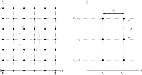
For the numerical solution of the system of ODEs (18.12), we can use a time-discretization scheme by introducing a temporal mesh ti = i δt, i = 0, 1,..., m with a mesh size δt:=Tm. Using different time discretizations, we derive three computational schemes, namely, the explicit Euler method, the implicit Euler method, and the Crank–Nicolson method. Applying one of these three schemes, we obtain a fully discretized approximation solution
ui,j≈uj(ti)≈u(tj,xj),i=0,1,...,m,j=0,1,...,n+1,
defined on the two-dimensional temporal-spatial mesh (see Figure 18.2). This is called a mesh solution to the IBV problem (18.9).
The Explicit Method
The explicit Euler method is obtained by replacing the time derivative by a forward finitedifference approximation. For a continuously differentiable function f, we have
df(t)dt=f(t+δt)−f(t)δt+O(δt).
Applying this formula for ∂u∂t in (18.10) gives
u(ti+1,xj)−u(ti,xj)δt=c2u(ti,xj−1)−2u(ti,xj)+u(ti,xj+1)δx2+O(δt+δx2) (18.15)
for each i = 0, 1,..., m − 1 and j = 1, 2,..., n. Discarding the error term O(δt+δx2) and replacing every u(ti, xj) by its approximation ui, j, we obtain the following finite-difference approximation to the heat equation (18.8):
ui+1,j=αui,j−1+(1−2α)ui,j+αui,j+1,i=1,2,...,n,j=0,1,...,m−1, (18.16)
where α:=c2δtδx2. The explicit method starts with the values u0, j (for i = 0), which are given by the initial time condition:
u0,j=f(xj),j=0,1,...,n+1. (18.17)
Additionally, the values ui,0 and ui,n+1 for all i = 1, 2,..., m are known thanks to the boundary conditions:
ui,0=g0(ti),ui,n+1=g1(ti),i=1,2,...,m. (18.18)
The formula (18.16) is an explicit expression for every approximation ui+1, j at time ti+1 in terms of the solution at the previous time ti. Therefore, this method is called the explicit Euler method. For a fixed i, the values ui+1, j for all j = 0, 1,..., n + 1 are computed from the values {ui, j}j = 0,1,..., n+1 of the ith time level. So the explicit rule (18.16) allows us to advance from the ith time level to the (i + 1)st time level. The accuracy of the explicit method is O(δt+δx2).
The explicit method (18.16) can also be written in matrix-vector form. Let us denote u(i) := [ui,1, ui,2, ..., ui,n]T. For each i = 0, 1, 2,..., m, the vector u(i) is an approximation to u(ti). Inserting the forward finite-difference approximation of the time derivative du(t)dt,
du(t)dt|t=ti=u(ti+1)−u(ti)δt+O(δt)≈u(i+1)−u(i)δt,
into Equation (18.12) written at t = ti gives
u(i+1)−u(i)δt=−c2δx2Au(i)+c2δx2g(ti),
which leads to the matrix-vector equations
u(i+1)=(In−αA)u(i)+αg(i),i≥0, (18.19)
where In denotes the n-by-n identity matrix and g(i) := g(ti). The formula (18.19) is an iterative rule which starts at
u(0)=f. (18.20)
The problem (18.19)-(18.20) admits a closed-form solution
u(k)=(In−αA)kf+αk−1∑i=1(In−αA)k−i−1g(i),0≤k≤m.
The Implicit Method
To derive the implicit method, we replace the time derivative of the solution by a backward finite-difference approximation:
df(t)dt=f(t)−f(t−δt)δtO(δt).
Applying this formula for ∂f(t)∂t in (18.10) gives
u(ti+1,xj)−u(ti,xj)δt=c2u(ti+1,xj−1)−2u(ti+1,xj)+u(ti+1,xj+1)δx2+O(δt+δx2) (18.21)
for each i = 0, 1,..., m − 1 and j = 1, 2,..., n. Discarding the error term O(δt+δx2) and replacing every u(ti, xj) by its approximation ui, j, we have
−αui+1,j−1+(2α+1)ui+1,j−αui+1,j+1=ui,j,i=1,2,...,n,j=0,1,...,m−1, (18.22)
subject to the initial condition (18.17) and boundary condition (18.18). As is seen from (18.22), the approximations ui+1,j of the (i + 1)st time level are coupled and cannot be calculated explicitly from approximations ui,j of the ith time level. Hence, this scheme is called the implicit method.
The implicit method (18.22) can be written in matrix-vector form. Inserting the backward finite-difference approximation of the time derivative du(t)dt,
du(t)dt|t=ti+1=u(ti+1)−u(ti)δt+O(δt)≈u(i+1)−u(i)δt,
into Equation (18.12) written at t = ti+1 gives
u(i+1)−u(i)δt=−c2δx2Au(i+1)+c2δx2g(i+1).
As a result, we obtain the following computational formula:
(In+αA)u(i+1)=u(i)+αg(i+1),i≥0, (18.23)
subject to the initial condition (18.20). The order of approximation is O(δt+δx2) which is the same as that of the explicit method.
To advance to the (i + 1)st time level and find the mesh solution u(i+1), we need to solve a system of linear equations with a tridiagonal coefficient matrix C = In + αA. In general, the numerical solution of a system with n equations and a band coefficient matrix requires O(n) operations. So the linear system Cx = b for x = u(i+1) with the tridiagonal matrix C and vector b = u(i) + αg(i+1) can be solved by the Gaussian elimination method with n − 1 eliminations (during the forward step) and n − 1 substitutions (during the backward step).
The Crank–Nicolson Method
The Crank–Nicolson method is one of the most well-known implicit finite-difference methods thanks to its stability properties and high order of approximation. To derive the Crank– Nicolson method, we first approximate the time derivative of u(t) at point t = ti + δt/2 with the central finite-difference formula that has the second order of approximation:
u(ti+1)−u(ti)δt+O(δt2)=du(t)dt|t=ti+δt/2=−c2δx2Au(ti+δt/2)+c2δx2g(ti+δt/2).
Second, we use the average of the spatial approximations at times ti+1 and ti in the right-hand side of the above equation:
u(ti+1)−u(ti)δt=−c22δx2A(u(ti)+u(ti+1))+c22δx2(g(ti)+g(ti+1))+O(δt2+δx2).
As a result, we obtain the following computational scheme, called the Crank–Nicolson method:
(In+α2A)u(i+1)=(In−α2A)u(i)+α2(g(i)+g(i+1)),i≥0. (18.24)
The method starts with the initial condition (18.20). As is seen from (18.24), the Crank– Nicolson method is an implicit computational scheme since we need to solve a system of linear equations to advance the mesh solution. However, the order of approximation of the Crank–Nicolson method is O(δt2+δx2), which is higher than the order of approximation of both explicit and implicit Euler methods. Additionally, the Crank–Nicolson method is unconditionally stable, meaning that it is not sensitive to roundoff errors regardless of the values of the mesh sizes δt and δx.
18.1.2.4 Stability Analysis
The stability of a computational method is closely associated with numerical errors. A finite-difference scheme is stable if the roundoff error made at one iteration does not amplify as the computations are continued. That is, if the errors decay or remain bounded, the numerical method is stable. If, on the contrary, the errors grow with time, the numerical method is said to be unstable. To investigate the stability of the explicit and implicit Euler methods and the Crank-Nicolson scheme, we represent them in the form of an iteration rule:
u(i+1)=Qu(i)+c(i),i≥0, (18.25)
where
Q={In−αA(the explicit method)(In+αA)−1(the implicit method)(In+α2A)−1(In−α2A)(the Crank-Nicolson method)c(i)={αg(i)(the explicit method)α(In+αA)−1g(i+1)(the implicit method)α2(In+αA)−1(g(i)+g(i+1))(the Crank-Nicolson method)
Let e(0) be the error introduced to the method initially. That is, in actual computations we start with the vector ũ(0) = u(0) + e(0), which includes the introduced error. Of interest is the propagation of this error during computations as we advance the solution in time. Let ũ(i) denote the mesh solution (of the ith time step) that includes the error. This perturbed mesh solution satisfies the rule (18.25):
˜u(i+1)=Q˜u(i)+c(i).
Subtracting (18.25) from this equation gives us the following recurrence formula for the accumulated error e(i) := ũ(i) − u(i):
e(i+1)=Q˜u(i)−Qu(i)=Qe(i).
Hence, the error at the kth time step is
e(k)=Qke(0),k≥0. (18.26)
Since the approximation error is a vector, we need matrix and vector norms to measure the magnitude of the error. Examples of matrix norms include
- ||Q||∞ := maxi∑j | Qij | = ||Q┬||1 (the biggest row-sum of magnitudes);
- ||Q||1 := maxj∑j | Qij | = ||Q┬||∞ (the biggest column-sum of magnitudes);
- ||Q||2:=√λmax (QΤQ) (the spectral norm given by the square root of the largest eigenvalue of the positive-semidefinite matrix Q┬Q).
Here Q is an n-by-n matrix of real elements Qij. Recall that a matrix norm || · ||* on ℝn×n is said to be compatible with a vector norm || · || on ℝn if
||Qx||≤||Q||*⋅||x||
holds for all Q ∈ ℝn×n and all x ∈ ℝn.
According to the definition given in the beginning of this subsection, a finite-difference method with the coefficient matrix Q is stable if the errors decay during the computations. For the error e(k) to decay and eventually vanish as k → ∞, that is, limk→∞ ||e(k) || = 0, it is necessary and sufficient that
||Qk||*<1 (18.27)
for some matrix norm ||· ||* and some positive integer K. Indeed, using properties of matrix and vector norms and the representation (18.26), we obtain
0≤||e(k)||≤||Q||b*⋅||Qk||a*⋅||e(0)||, (18.28)
where the nonnegative integers a and b < K are defined so that k = a· K + b. Provided that (18.27) holds, the right-hand side of (18.28) converges to 0 as k→ ∞. Note that if QK ||* = 1, then the errors remain bounded as k→ ∞, i.e., lim supk→∞ ||e(k) || <∞.
The stability condition can be formulated with the use of the spectral radius. The spectral radius ρ(Q) of an n-by-n matrix Q is defined by the maximum magnitude of the eigenvalues λ1,λ2,...,λn of Q. That is,
ρ(Q):=max{|λ1|,|λ2|,...,|λn|}.
Note that for a symmetric matrix, the 2-norm is equal to the spectral radius of the matrix, i.e.,||Q||2 = ρ(Q) if Q = QT.
A finite-difference method is stable if the spectral radius of the matrix Q be less than one, i.e.,
ρ(Q)<1. (18.29)
Proof. Let us prove that the conditions (18.27) and (18.29) are equivalent. First, use the fact that the spectral radius does not exceed ||Qk||1/k* for any matrix norm || · ||* and any positive integer k. That is, ρ(Q)≤||Qk||1/k*. Therefore, ||Qk||* < 1 implies that ρ(Q) < 1. On the other hand, according to Gelfand’s formula, for any matrix norm || · ||* we have lim k→∞||Qk||1/k*=ρ(Q). Let ρ(Q) = α0 < 1. Then, there exists k so that we have
|||Qk||1/k*−ρ(Q)|<1−α02⇒||Qk||1/k*<ρ(Q)+1−α02=1+α02<1.
Stability Analysis of the Explicit Method
Let us calculate the spectral radius of Q = In − αA, where α=c2δtδx2>0 and A is given by (18.14). Let λ be an eigenvalue of A and x be a respective eigenvector, i.e., Ax = λx holds.1 We have
Qx=(In−αA)x=Inx−αAx=x−αλx=(1−αλ)x.
That is, all eigenvalues of the matrix Q are of the form μ = 1 − αλ. Therefore, to calculate ρ(Q) we only need to know the smallest and largest eigenvalues of the matrix A.
The eigenvalues of the n-by-n matrix A defined by (18.14) are
λj=2−2cos θj,
which are associated with the respective n-by-1 eigenvectors
xj=[sin (θj),sin (2θj),...,sin (nθj)]Τ, (18.30)
where θj=jπn+1 for all j = 1, 2,..., n.
Proof. It is left as an exercise for the reader to verify this.
Due to Proposition 18.3, the eigenvalues of Q are
μj=1−αλj=1−α(2−2cos θj)=1−4αsin 2(jπ2(n+1)),j=1,2,...,n.
Hence, the stability requirement, ρ(Q) = maxj|μj| < 1, can be written as follows:
−1<1−4αsin 2(jπ2(n+1))<1,j=1,2,...,n.
Since α > 0, the right inequality is automatically satisfied. Rearranging the left inequality gives
12>αsin 2(jπ2(n+1)),j=1,2,...,n.
The sequence {sin 2(jπ2(n+1));j=1,2,...,n} attains its maximum value at j = n. The maximum approaches 1 from below as n→ ∞. Thus, the above restrictions on α are satisfied for any n ≥ 1 iff α≤12. To insure the stability of the explicit method, we require that
c2δtδx2≤12 (18.31)
holds. The explicit method is said to be conditionally stable. The condition (18.31) can also be interpreted as follows: every time we double the number of mesh points along the x-axis (and hence halve the mesh size δx), we need to quadruple the number of mesh points along the t-axis.
The stability of an explicit finite-difference method can also be investigated using the matrix norm. The explicit Euler method is stable if ||Q||* ≤ 1 for some norm || · ||*. Calculating the biggest row-sum of magnitudes of Qij we have
||Q||∞=|1−2α|+2|α|.
If α>12, then ||Q||∞ = 4α − 1 > 1 and the scheme is unstable. If α≤12, then ||Q||∞ = 1 and the scheme is stable.
Stability Analysis of the Implicit Method
The eigenvalues νj of the matrix In + αA can be calculated from those of A as follows:
νj=1+αλj=1+4αsin 2(jπ2(n+1)),j=1,2,...,n.
All of them are strictly greater than one. In particular this fact ensures that the inverse Q = (In + αA)−1 exists. Since Q is a nonsingular matrix, its eigenvalues μj are reciprocals of the eigenvalues νj of In + αA. Therefore, the implicit method is stable since
0<11+4αsin 2(jπ2(n+1))<1
for all j = 1, 2,..., n and for all α > 0. The implicit method is said to be unconditionally stable since there is no restriction on the choice of the mesh sizes δx and δt.
Stability Analysis of the Crank–Nicolson Method
An important observation is that the matrices B≡In+α2A and C≡In−α2A have the same eigenvectors as those of the matrix A. The eigenvalues νBj of B and νCj of C associated with the eigenvector xj defined by (18.30) are, respectively, given by
νBj=1+α2λj and νCj=1−α2λj.
Moreover, since α > 0, all eigenvalues of B are strictly positive; in fact, they all lie in the interval (1, 1+ α). Hence the matrix B is nonsingular. The eigenvalues of the inverse B− 1 are of the form 1νBj since
Bxj=νBjx⇔1νBjxj=B−1xj.
Therefore, the eigenvectors of Q = B−1C are the same as those of A. The eigenvalues μj of Q are
μj=1−α2λj1+α2λj=1−2αsin 2(jπ2(n+1))1+2αsin 2(jπ2(n+1))
for j = 1, 2,..., n. Indeed, we have
Qxj=B−1(Cxj)=νCjB−1xj=νCjvBjxj.
The magnitude of every eigenvalue μj is strictly less than one. Therefore, the Crank– Nicolson method is unconditionally stable.
18.2 Pricing European Options
Valuation of a European derivative is probably the most elementary problem of computational finance. In the case of a single asset price model, this problem reduces to the numerical evaluation of a one-dimensional integral. Hence, the result can be achieved with the use of quadrature rules. On the other hand, according to the risk-neutral pricing formula, the no-arbitrage derivative value is the expected value of the discounted payoff function. The mathematical expectation can be evaluated by the Monte Carlo method, which is especially efficient for pricing basket (i.e., multi-asset) options and path-dependent derivatives, the numerical evaluation of which is discussed in later sections. The PDE formulation of the derivative price problem allows for the application of finite-difference schemes. Finally, we may use multinomial tree methods (also known as lattice methods) that can be derived as a result of a discrete-time approximation of a continuous-time asset price model. In fact, tree methods are closely related to Monte Carlo methods. Furthermore, they can also be considered as a special case of explicit finite-difference methods.
18.2.1 Pricing European Options by Quadrature Rules
Let us consider a standard European-style option maturing at time T with payoff function Λ(S(T)), where S(T) is the time-T price of the underlying asset. Here, we assume that the underlying price process {S(t)}t≥0 is time homogeneous and Markovian and that the (risk-neutral) probability law of the price S(T) conditional on S(t) = S for 0 ≤ t < T is known. We can therefore express the option value v(τ, S) as function of the time to maturity τ = T − t and spot S = S(t). As we have seen in previous chapters, the no-arbitrage option value is given by the risk-neutral pricing formula and can be evaluated as a one-dimensional integral (using the risk-free bank account B(t) = ert as numéraire):
υ(τ,S)=e−rT˜Et,S[Λ(S(T))]=e−rT∫∞0Λ(S′)˜p(τ;S,S′)dS′ (18.32)
Here, ˜p(τ ; S, S′) denotes the risk-neutral transition PDF of the asset price process. Some examples of processes for which the PDF ˜p is known in closed form include the log-normal (GBM) model and the constant elasticity of variance (CEV) diffusion model. There are also other interesting families of more generally state-dependent nonlinear volatility diffusion models that admit analytically closed-form expressions for the transition PDF. Some jump-diffusion processes such as the variance gamma (VG) model and the normal inverse Gaussian (NIG) model, which are constructed from Brownian motion with the use of a stochastic time change, also admit transition PDFs in closed form.
We can also compute the Greeks of the contract such as the delta Δ(τ,S)=∂υ∂S(τ,S). Provided that we can change the order of integration and differentiation and that the integrals obtained exist, we have
Δ(τ,S)=e−rT∂∂S∫∞0Λ(S′)˜p(τ;S,S′)dS′=e−rT∫∞0Λ(S′)∂˜p∂S(τ;S,S′)dS′. (18.33)
In some cases, the integrals in (18.32)–(18.33) can be computed in closed form. Explicit formulas for the Greeks in the case of the log-normal (GBM) asset price model were derived in previous chapters. In general, we rely on numerical methods. The integral in (18.32) can be computed with the use of quadrature formulae like those of Subsection 18.1.1:
υ(τ,S)≈e−rTn∑i=1wiΛ(si)˜p(τ;S,si),
where the summation is taken over a set of nodes s1, s2,..., sn ∈ ℝ+. The integral in (18.32) is an improper one. To use a quadrature formula, we can first apply a change of variables to transform the integration interval into a finite one. Alternatively, we can truncate the integration region and integrate the function Λ(S′)˜p(τ ; S, S′) w.r.t. S′ over a bounded interval (0,Smax). One case is where the payoff Λ is nonzero on a finite interval such as the put option payoff Λ(S′) = (K − S′)+ = (K − S)?{S′≤K}. If Λ(S′) = 0 for all S′ ≥ K, then we take Smax = K. In many other cases we may observe that the integrand goes to zero exponentially fast as S′→ ∞. If this is the case, then for any given ε > 0 one can find Smax > 0 such that ∫∞Smax Λ(S′)˜p(τ;S,S′)dS′<ε.
Let us calculate the initial (set t = 0) value of a European call option under two asset price models that are more involved than the GBM model, namely, the constant elasticity of variance (CEV) diffusion model and the geometric variance gamma (GVG) model. First, we need to identify the transition probability density of each asset price process. Second, we apply a quadrature rule to evaluate the integral (18.32), which can be written for the case with the European call option with time to maturity T , strike price K, and spot S0 as
υ(T,S0)=e−rT∫∞0Λ(S)˜p(T;S0,S)dS (18.34)=e−rT∫∞K(S−K)˜p(T;S0,S)dS. (18.35)
In the following calculations, we assume that the risk-free interest rate r is 5%, the dividend yield q is 0, the initial asset price S0 is 100, and the time to maturity T is 0.5 (years).
(Option Pricing in the CEV model). Consider the CEV diffusion model {S(t) ∈ ℝ+}t≥0, which follows
dS(t)=νS(t)dt+αS(t)β+1d˜W(t) (18.36)
with real constants α > 0, β, ν = r − q and where {˜W(t)}t≥0 is a standard Brownian motion in a risk-neutral measure ℙ. The local volatility is a nonlinear (power) function: σ(S)/S = αSβ. We consider the case with β < 0. Hence, the origin is attainable in finite time, i.e., the stock can attain a zero price in finite time. In particular, the origin is an exit boundary for β ∈ [−1/2, 0) and it is a regular boundary (which we specify as killing) for β < − 1/2. Note that the discounted process {e−νtS(t)}t≥0 is ℙ-martingale. For numerical illustration, we take the following parameter values: β =−2 and α = 2500. The instantaneous volatility at S0 = 100 is αSβ0=25001002=25%. The transition density has the known explicit representation
˜p(t;S0,S)=e−νt(e−νtS)−2β−32S120α2|β|τte−(e−νtS)−2β+S−2β02α2β2τtI12|β|((e−νtS)−βS−β0α2β2τt), (18.37)
for S0,S, t > 0, τt=12νβ(e2νβt−1) if ν ≠ 0 and τt = t if ν = 0. This PDF involves Iα(z) which is the modified Bessel function of the first kind of order α and argument z.
To simplify our calculations, we recall how the above CEV process is related to the simpler known squared Bessel process (SQB){X(t) ∈ ℝ+}t≥0 with index μ≡ 1/(2β) and having the transition PDF
pu(t;x0,x)=(xx0)μ2e−(x+x0)/2t2tI|μ|(√xx0/t). (18.38)
By defining the invertible smooth mapping X: ℝ+→ ℝ+
Χ(S):=S−2β/(α2β2)=S2|β|/(α2β2),
with inverse X− 1(x)≡ F(x) := (α2β2x)1/2|β|, we obtain the driftless, i.e., ν = 0, CEV process {S(0)(t) := F(X(t)), t ≥ 0}. The CEV processes with and without drift are simply related by a scale and time change:
S(t)=eνtS(0)(τt)=eνtF(X(τt)). (18.39)
It can be verified that the risk-neutral transition PDF of the CEV process, ˜p, is related to that of the SQB process as
˜p(t;S0,S)=e−νt|Χ′(e−νtS)|pμ(τt;Χ(S0),Χ(e−νtS)). (18.40)
By substituting the expression in (18.38) for pμ, we see that (18.40) is exactly Equation (18.37).
Using (18.40), for t = T and ν = r, and changing integration variables with S = erT F(x), x = X(e−rT S), and dS=erTΧ′(F(x))dx,, the integral in (18.35) takes the form
υ(T,S0)=∫∞Χ(e−rTK)(F(x)−e−rTK)pu(τT;Χ(S0),x)dx, (18.41)
where μ=12β. This is an improper integral over a half-line which can be transformed into an integral over a finite interval by a change of variables. For example,
∫∞af(x)dx=∫10f(a+y1−y)dy(1−y)2. (18.42)
To compute the call price, the integral in (18.41) is transformed as in (18.42) where
a=Χ(e−rtK) and f(x)=(F(x)−e−rTK)pμ(τT;Χ(S0),x).
Alternatively, we can first evaluate the corresponding European put option (with same strike and maturity) and then obtain the call option value with the use of the put-call parity. The evaluation of a put option reduces to computing the integral (18.34) with Λ(S) = (K − S)+ over a finite interval (0, K).
With the above chosen model parameters, we employ Romberg integration with 101 initial nodes and four improvements. First, we evaluate the call option with strike K = 100. The output of the Romberg method is in shown Table 18.3, where the best approximation for the definite integral is the bottom rightmost boxed entry. The approximation error is given by the magnitude of the difference between the diagonal elements in the two bottom rows of the table. Second, we evaluate the call option for strikes K ∈ {90, 100, 110} and compare the results obtained with the call option values calculated under the GBM model with volatility σ = 0.25 (see Table 18.4). For comparison, we also calculated the Black–Scholes implied volatility for the CEV call option values. As is seen, the implied volatility is a decreasing function of strike K.
Application of the Romberg numerical integration method to pricing a European call option with T = 0.5 and K = 100 under the CEV model. The approximation error is estimated at 1.057 · 10−11.
8.2978647600469 | ||||
8.2978711263121 |
8.2978732484004 | |||
8.2978727104861 |
8.2978732385441 |
8.2978732378870 | ||
8.2978731065344 |
8.2978732385506 |
8.2978732385511 |
8.2978732385616 | |
8.2978732055469 |
8.2978732385510 |
8.2978732385511 |
8.2978732385511 |
8.2978732385510 |
Comparison of the call values computed under the Black–Scholes (GBM) model and the CEV model for different strikes. The implied Black–Scholes volatility (Impl. BS Vol.) is computed for the CEV option values.
Strike K |
Call Value under GBM |
Call Value under CEV |
Impl. BS Vol. |
|---|---|---|---|
90 |
14.437116236461 |
15.033304012884 |
27.89% |
100 |
8.260015199343 |
8.297873238551 |
25.14% |
110 |
4.225782392960 |
3.642151895619 |
22.81% |
(Pricing in the GVG model). The variance gamma (VG) process {X(t)}t≥0 is obtained by evaluating a scaled Brownian motion with drift W (θ,σ)(t) at a random time given by a gamma process G(t):
X(t):=W(θ,σ)(G(t))=θG(t)+σW(G(t)), t≥0.
Recall that the gamma process is characterized by two positive parameters, μ and υ. The parameter μ controls the rate of jump arrivals and the scaling parameter υ inversely controls the jump size. It is assumed that the process starts from 0 at time 0. The marginal distribution of a gamma process at time t is a gamma distribution with shape parameter μtυ and rate parameter 1υ. The mean and variance of G(t) are, respectively, μtυ and μtυ2. In the VG model, the parameter μ is set to 1 thus G(t) ~ Gamma (tυ,1υ).
The risk-neutral asset price dynamics is given by the geometric variance gamma (GVG) process as
S(t)=S0e(r−q+w)t+X(t),
where ω=1υln (1−θυ−σ2υ/2) is a correction constant ensuring that the mean rate of return on the asset is r − q. The risk-neutral transition probability distribution is a mixture of the normal and gamma probability distributions. The PDF of Z(t) := ln(S(t)/S(0)) is given by
pz(t)(z)=2eθx/σ2υt/υ√2πσΓ(t/υ)(x22σ2/υ+θ2)t2υ−14Ktυ−12(|x|σ2√(2σ2/υ+θ2)), (18.43)
for all t > 0, z ∈ ℝ, where Γ is the gamma function, Kα is the modified Bessel function of the second kind of order α, and x = z − (r − q)t − ωt. Since the asset price is given by an exponential of the log price ratio Z(t), i.e., S(t) = S0eZ(t), the value of a European option maturing at time T with payoff Λ(S) is given by
υ(T,S0)=e−rT∫∞−∞Λ(S0ez)pz(T)(z)dz. (18.44)
For a standard European call with strike K we have
υ(T,S0)=e−rT∫∞ln (K/S0)(S0ez−K)pz(T)(z)dz.
By using the transformation in (18.42), we can change the semi-infinite interval into the finite interval (0, 1) and then apply Romberg integration to evaluate the European call with K = 100. For numerical illustration, we take parameter values from Madan et al. (1998): θ = 0.1436, σ = 0.12136, and υ = 0.3. The other parameters are the same as those in the previous example. The output of Romberg method is given in Table 18.5, where the best approximation for the definite integral is the bottom rightmost boxed value.
Application of the Romberg numerical integration method to pricing a European call option with T = 0.5 and K = 100 under the GVG model. The approximation error is estimated at 8.663 · 10−15.
5.0807555357638 | ||||
5.0835997925475 |
5.0845478781420 | |||
5.0843105384813 |
5.0845474537926 |
5.0845474255026 | ||
5.0844882050319 |
5.0845474272154 |
5.0845474254436 |
5.0845474254426 | |
5.0845326204230 |
5.0845474255534 |
5.0845474254426 |
5.0845474254426 |
5.0845474254426 |
Algorithm 18.1 The Monte Carlo Method for Estimation of the No-Arbitrage Value of a European-Style Contract.
- Sample n i.i.d. asset prices {Sk}k = 1,2,..., n from the probability distribution of S(T) conditional on S(0) = S0. Calculate the sample values of the discounted payoff function: Λk := e−rT Λ(Sk) for k = 1, 2,..., n.
- Compute the sample estimate for the price V0 = v(T, S0) = Ẽ[e−rT Λ(S(T))]:
V0≈ˉΛn:=1nn∑k=1Λk.
- Construct an asymptotically valid 100(1 − α)% confidence interval for V0:
(ˉΛn−zα/2σn,ˉΛn+zα/2σn)∍V0,
where zα/2 is the upper (1 − α/2)-quantile of the standard normal distribution, σn=sn/√n is the stochastic error, and s2n=1n∑nk=1Λ2k−(ˉΛn)2 is the sample variance.
Algorithm 18.2 Simulation of the CEV Diffusion Model with Absorption at the Origin.
input S0 > 0, T > 0, β < 0, α > 0, ν = r − q
set μ←12β,X0←S−2β0α2β2,τ←{12νβ(e2νβT−1),ν≠0,T,ν=0,pa←Γ(|μ|,X02τ))/Γ(|μ|)
generate U ← Unif(0, 1)
if U > pa then
generate Y←IΓ(|μ|,X02τ),X←Gamma(Y,12τ)
else
set X ← 0
end if
return S(T) ← eνT (α2β2X)− 0.5/β
18.2.2 Pricing European Options by the Monte Carlo Method
Let{S(t)}t≥0 be a stochastic asset price process starting at S0. Suppose that it can be simulated exactly from its transition distribution. The no-arbitrage price v(T, S0) of a European-style contract with the time to maturing T > 0 and payoff Λ(S(T)) can be estimated by the Monte Carlo method as described in Algorithm 18.1.
To illustrate the use of the Monte Carlo algorithm, we apply Algorithm 18.1 to the CEV diffusion asset price model, the geometric variance gamma pure jump model, and a multidimensional geometric Brownian motion model.
(Pricing Options under the CEV Diffusion Model). The Monte Carlo simulation of the constant elasticity of variance (CEV) diffusion process that follows the SDE (18.36) is based on the reduction of its transition probability distribution to one of the randomized gamma distributions studied in Chapter 17. Assume the risk-neutral probability measure so that ν = r − q in (18.36). Recall from (18.39) that the CEV diffusion
Estimation of the standard European call option value. The MCM estimate, respective standard stochastic error σn=sn/√n, and 95% confidence interval are reported for several values of the sample size n. Computations are performed for K = 100 and T=12 under the CEV model with parameters as specified in Example 18.3.
{S(t)}t≥0 can be represented as a function of a time-changed SQB process {X(t)}t≥0:
S(t)=eνt(α2β2X(τt))−1/2β, where τt={12νβ(e2νβt−1),ν≠0,t,ν=0, (18.45)
Again, we consider the case with β < 0 so that the origin is an exit for β ∈ [−1/2, 0) and specified as a killing regular boundary in the case β < − 1/2. The CEV model reduces to the SQB process as given in (18.45). First, Algorithm 17.13 is used to sample the value X(τt) of the SQB process. Second, the terminal stock value S(T) of the CEV process is obtained by applying the mapping (18.45) with t = T . As a result, we obtain Algorithm 18.2, which returns the sample value of S(T) (for T > 0) conditional on S(0) = S0 > 0.
In the Monte Carlo experiment, we estimate the initial value of a European call option with maturity T=12 and strike price K = 100. The CEV model parameters used here are the same as those in Example 18.3. In Table 18.6 we report the Monte Carlo estimate, standard error, and 95% confidence interval computed for several values of the sample size n. Figure 18.7 demonstrates the convergence of the sample estimate to the exact value of the call option as n increases.
Size n |
MCM Estimate |
Stoch. Error σn |
95% Confidence Interval |
|---|---|---|---|
20,000 |
8.35181 |
0.14084 |
(8.21097, 8.49265) |
40,000 |
8.25013 |
0.09896 |
(8.15117, 8.34908) |
60,000 |
8.20935 |
0.08049 |
(8.12886, 8.28984) |
80,000 |
8.24294 |
0.06985 |
(8.17309, 8.31280) |
100,000 |
8.24361 |
0.06241 |
(8.18120, 8.30602) |
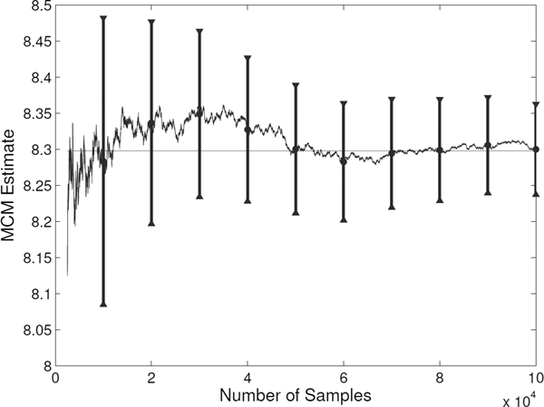
Convergence of the unbiased Monte Carlo estimate to the exact price of the European call option (represented by a horizontal line) as the sample size n increases. For each value of n equal to a multiple of 104, the 95% confidence interval is constructed. Computations are performed for K = 100 and T=12 under the CEV model with parameters as specified in Example 18.3.
(Pricing Options under the Variance Gamma Model). The simulation of the VG process relies on sampling normal and gamma random variables. To simulate X(t) = B(G(t)) at some time t > 0, we first sample the gamma time G(t)~ Gamma(t/ν, 1/ν) and then sample a Brownian increment B(g)~ Norm(θg,σ2 g) given g = G(t). Thus, we can express the GVG asset price S(T) at maturity T (under the risk-neutral measure) as a function of independent gamma and normal random variables:
S(T)d=S0e(r−q+w)T+θG/ν+σ√G/νZ,where Z~Norm(0,1) and G~Gamma(T/ν,1).
In the Monte Carlo experiment, we estimate the value of a European call option with maturity T=12 and strike price K = 100. The GVG model parameters used here are the same as those in Example 18.4. In Table 18.8 we report the Monte Carlo estimate, standard error, and 95% confidence interval computed for several values of the sample size n. Figure 18.9 demonstrates the convergence of the sample estimate to the exact value of the call option as n increases.
Estimation of the standard European call option value. The MCM estimate, respective standard stochastic error σn=sn/√n, and 95% confidence interval are reported for several values of the sample size n. Computations are performed for K = 100 and T=12 under the GVG model with parameters as specified in Example 18.4.
Size n |
MCM Estimate |
Stoch. Error σn |
95% Confidence Interval |
|---|---|---|---|
20,000 |
5.06430 |
0.12338 |
(4.94091, 5.18768) |
40,000 |
5.03148 |
0.08679 |
(4.94469, 5.11827) |
60,000 |
5.06728 |
0.07091 |
(4.99637, 5.13819) |
80,000 |
5.07949 |
0.06160 |
(5.01789, 5.14109) |
100,000 |
5.10104 |
0.05521 |
(5.04583, 5.15624) |

Convergence of the unbiased Monte Carlo estimate to the exact price of the European call option (represented by a horizontal line) as the sample size n increases. For each value of n equal to a multiple of 104, a 95% confidence interval is constructed. Computations are performed for K = 100 and T=12 under the GVG model with parameters as specified in Example 18.4.
(Pricing Basket Options under the Multi-Asset GBM Model). Consider the pricing of derivative contracts under an N-asset GBM model with M Brownian factors. Let us recall the risk-free dynamics of the ith asset price described by
Si(t)=Si(0)exp ((r−qi−σ2i/2)t+σiM∑j=1ℓij˜W(t)),t≥0,
where σi is the volatility of the ith asset, qi is the dividend yield on the ith asset, {˜Wj(t)}t≥0 are i.i.d. Brownian motions (within the assumed risk-neutral measure ˜ℙ) labelled by j = 1, 2,...,M, and the coefficients ℓij are chosen so that ∑Mj=1ℓ2ij=1 for all i = 1, 2,...,N. For each i = 1, 2,...,N, the log-return Xi(t):=ln (Si(t)Si(0)) is a normal random variable with mean (r−qi−σ2i/2)t and variance σ2it. The joint distribution of the log-returns X1(t),X2(t) ...,XN (t) is multivariate normal with N-by-N correlation matrix ρ = LLT, where L is an N-by-M matrix with entries ℓij. The covariance among the log-returns is given by the N-by-N matrix with entries
Cov(Xi(t),Xj(t))=tΣij where Σ=DρD and D=diag(σ1,σ2,...,σN).
Consider a multi-asset (basket) European derivative contract with time to maturity T and payoff Λ (S1(T),S2(T),...,SN (T) . We have priced some examples of such options, including options on the maximum with payoff maxi{wiSi(T)}, or the minimum with payoff mini{wiSi(T)}, etc., where w1, w2,..., wN are positive coefficients. Given time-0 spot values Si(0) = si > 0, i = 1, 2,...,N, the initial no-arbitrage value of this derivative is
V(s1,s2,...,sN;T)=e−rT˜E0[Λ(S1(T),S2(T),...,SN(T))|Si(0)=si,1≤i≤N].
For large values of N and M, we can only rely on Monte Carlo methods for pricing. To apply Algorithm 18.1, we need to generate n i.i.d. sample values of the payoff function. The completion of part 1 in Algorithm 18.1 involves the following three steps:
- i. Sample n× M i.i.d. random variables Z(k)j, 1 ≤ k ≤ n, 1 ≤ j ≤ M, from the standard normal distribution.
- ii. For each i = 1, 2,...,N, obtain n sample values of the terminal stock value Si(T),
S(k)i=siexp ((r−qi−σ2i/2)T+σi√TM∑j=1ℓijZ(k)j),k=1,2,...,n.
- iii. Calculate the sample values of the discounted payoff function
Λk=e−rTΛ(S(k)1,S(k)2,...,S(k)N),k=1,2,...,n.
18.2.3 Pricing European Options by Tree Methods
Assume a log-normal model for stock prices in an economy with fixed interest rate r and zero stock dividend. Recall that under the risk-neutral measure ˜ℙ with ˜W as standard Brownian motion, the stock price has the representation
S(t)=S0e(r−σ2/2)t+σ˜W(t).
As was discussed in Chapter 2, the log-normal continuous-time model can be derived as a limiting case of discrete-time binomial tree models. Therefore, we can use a binomial tree to approximate the GBM dynamics. To guarantee a good order of approximation, the length of time periods has to be small enough. Multinomial tree models allow for improving both the accuracy and speed of the binomial method. In an n-nomial tree model, the stock price can jump to one of n possible branches over each time period. As a result, we can attain a higher order of approximation without having to increase the computational work by much.
18.2.3.1 Binomial Model
Consider a recombining binomial tree model with N + 1 trading dates tn = n δt, n = 0, 1,...,N uniformly spread throughout the interval [0, T] with step size δt=TN (i.e., the number of periods per year equals 1δt). The upward and downward factors, u and d, of the standard binomial tree model can be obtained by matching the first two moments of the stock price returns. The following solution is the most commonly used in binomial models:
u=eσ√δtand d=1u=e−σ√δt. (18.46)
The risk-neutral probability is given by the usual formula:
˜p=erδt−du−d. (18.47)
For this choice of parameters, the variances of a single period return in the continuous- and discrete-time models agree up to O(δt2). Note that other solutions for u, d, ˜p are possible; however, their analytical expressions are more cumbersome.
Consider the application of a binomial tree to pricing a European option with maturity T and payoff Λ(S). The continuous-time log-normal stock price process is approximated by a discrete-time binomial price process on the N-period lattice with the nodes Sn, k = S0undn − k, k = 0, 1,..., n and n = 0, 1,...,N. We calculate the option values Vn,k := V (n, Sn,k) using the backward-in-time recursion as follows.
- At maturity, set VN, k = Λ(SN, k) for each k = 0, 1,...,N.
- For each n = N − 1,N − 2,..., 0, compute the option values Vn, k as follows:
Vn,k=e−rδt(˜pVn+1,k+1+(1−˜p)Vn+1,k),k=0,1,...,n.
In this example, we study whether the binomial option price formula approximates the respective continuous-time solution with accuracy O(δt). Consider a butterfly option centred at 100 with the spread [80, 120]. The payoff is
Λ(S)={S−80if 80<S≤100,120−Sif 100<S<120,0if S≤80 or S≥120. (18.48)
Assume that the annual volatility σ is 0.25 and the annual risk-free rate of interest r is 0.05. Let us compute and compare the no-arbitrage prices and deltas of the butterfly option with T=12 for spot value S0 = 100 under the following asset price models:
- (a) the log-normal (GBM) model,
- (b) the binomial model with N = 50, 100, 200, 400 where u and d are given in (18.46).
The payoff of a butterfly option is equivalent to that of a portfolio in three standard European calls. In particular, the payoff in (18.48) is equivalent to a portfolio in one long call with strike 80, two short calls with strike 100, and one long call with strike 120. Therefore, the initial value and delta of a butterfly option with the payoff in (18.48) calculated under the log-normal model are, respectively,
V=CBS(K=80)−2CBS(K=100)+CBS(K=120),Δ=ΔBS(K=80)−2ΔBS(K=100)+ΔBS(K=120),
where CBS(K) and ΔBS(K) are, respectively, the Black–Scholes call value and call delta for strike K and the same maturity and spot value as those used to price the butterfly option. For T = 0.5 and S0 = 100, we have the following value and delta of the butterfly option under the GBM model:
V=7.97318602436266 and Δ=−0.0381920926996022.
The errors of binomial approximations are reported in Table 18.10. As is seen from the table, the binomial model approximation error is proportional to δt.
Errors of binomial approximations for the butterfly option value and delta.
N |
δt |
Price Error |
Delta Error |
|---|---|---|---|
50 |
0.001 |
0.08652 |
0.00013 |
100 |
0.0005 |
0.03047 |
0.00048 |
200 |
0.0025 |
0.01606 |
0.00022 |
400 |
0.00125 |
0.01018 |
0.00002 |
18.2.3.2 Multinomial Models
In the binomial model, the asset price can jump to one of two possible states in each time step. To improve the accuracy of option valuation, we allow a jump to multiple states for the asset price. Consider a European-style option with a payoff function Λ(S) and maturity date T > 0. The no-arbitrage option value V (t, S) as a function of (actual) calendar time t and spot S satisfies
V(t,S)=e−rδt˜E[V(t+δ,S(t+δt))|S(t)=S],0≤t<t+δt≤T. (18.49)
This equation can be used to recursively compute option prices
V(T−δt,⋅),V(T−2δt,⋅),...,V(0,⋅)
at every time t = n δt starting at maturity T , where V (T, S) = Λ(S), and then advancing backward in time until time 0 is reached. To make this approach feasible, we need to introduce a discrete grid in the spatial variable S and then approximate the mathematical expectation in (18.49) by a finite sum evaluated on the grid.
Let us fix the time step δt and introduce the time grid tn = n δt for n = 0, 1,...,N, where N=Tδt. For every period [tn, tn+1], the ratio of asset prices S(tn+1) and S(tn) is a function of the Brownian increment δ˜Wtn+1:=˜W(tn+1)−˜W(tn)~Norm(0,δt):
S(tn+1)S(tn)=e(r−σ2/2)δt+σδt˜Wtn+1.
Each Brownian increment δ˜Wtn is approximated by a discrete random variable δ˜Wn that takes values − b δx, − (b − 1) δ x,..., b δx with respective probabilities p− b, p− b+1,..., pb, summing to unity, where b ∈ ℕ is a branching parameter and δx > 0 is a mesh size. As a result, the Brownian motion {˜W(t)}t≥0 is approximated by a Markov chain {˜Wtn}n≥0, which is defined at discrete times tn = n δt, n ≥ 0, and takes discrete values k δx, k ∈ ℤ. For each time tn, the variable ˜Wtn is given by a sum of n i.i.d. increments,
˜Wtn=δ˜W1+δ˜W2+⋯+δ˜Wn;
it takes values in the set {k δx| k = − nb, − nb + 1 ,..., nb}. The value of ˜Wtn+1 conditional on ˜Wtn=kδx is in the set {(k − b) δx, (k − b +1) δx,..., (k + b) δx}. The process {˜Wtn}n≥0 is a random walk whose realizations are paths in a recombining multinomial tree. The tree is organized such that there are 2bn + 1 nodes at time tn and each node has 2b + 1 branches. By setting b equal to 1 or 2, we can obtain a trinomial or pentanomial tree, respectively. The latter is shown in Figure 18.11.

The approximation of the process {˜W(t)}t≥0 by {˜Wtn}n≥0 leads to an approximation of the continuous-time asset price process {S(t)}t≥0 by a discrete-time Markov chain {Stn}n≥0 defined by
Stn=exp ((r−σ2/2)tn+σ˜Wtn).
Denote the value of Stn at the node (n, k) of the multinomial tree by
Sn,k:=exp ((r−σ2/2)nδt+σkδx).
The conditional expectation in (18.49) can now be approximated as follows:
erδtV(tn,Sn,k)=˜E[V(tn+1,S(tn+1))|S(tn)=Sn,k]=˜E[V(tn+1,Sn,ke(r−σ2/2)δt+σδ˜Wtn+1)]≈˜E[V(tn+1,Sn,ke(r−σ2/2)δt+σδ˜Wtn+1)]≈b∑j=−bpjV(tn+1,Sn+1,k+j). (18.50)
This gives us the following computational scheme:
Vn,k=e−rδtb∑j=−bpjVn+1,k+j,n=N−1,N−2,...,0,k=−nb,−nb+1,...,nb
where Vn, k denotes the approximation of the option price V (tn,Sn,k) at the node (n, k). As usual, the option values at maturity T = N δt are given by the payoff function:
VN,k=Λ(SN,k),k=−Nb,−Nb+1,...,Nb.
To attain a high order of convergence in multinomial methods, the probabilities {pj; j = − b, − b + 1 ,..., b} should be chosen such that ˜Wtn is a good approximation of ˜W(tn). This can be achieved by using the moment matching method. According to Heston and Zhou (2000), if the first k moments of the Brownian increment δWn match those of δ˜Wtn=˜Wtn−˜Wtn−1, that is,
b∑j=−b(jδx)lpj=0,for all odd l≤k (18.51)
and
b∑j=−b(jδx)lpj=δtl/2l!2l/2(l/2)!,for all even l≤k, (18.52)
and if the terminal payoff function is 2k times continuously differentiable, then the multi-nomial approximation (18.50) has a local error of O(δt(k+1)/2), and the associated discrete-time solution converges to the continuous-time solution at a rate of O(δt(k−1)/2), that is,
V(tn,Sn,k)=Vn,k+O(δt(k−1)/2).
We can easily match all the odd moments by putting p−j = pj for all j. To match the first b even moments, we must solve the simultaneous equations
b∑j=02(jδx)2kpj=δtk(2k)!2kk!,k=1,2,...,b. (18.53)
Additionally, we require the probabilities pj to sum up to one,
p0+2b∑j=1pj=1. (18.54)
The left- and right-hand sides of (18.53) are, respectively, proportional to δx2k and δtk. Thus, if assume that δx=√aδt holds for some constant a > 0, then we can cancel out δx and δt in (18.53) to obtain
b∑j=02(ja)2kpj=(2k)!2kk!,k=1,2,...,b. (18.55)
Solving these equations, we find the probabilities pk that do not depend on δt or δx. The parameter a can be chosen to match an additional moment constraint
b∑j=12(ja)2b+2pj=(2(b+1))!2b+1(b+1)!⋅δtb+1. (18.56)
Combining (18.54), (18.55), and (18.56), we obtain the following matrix equation on the probabilities p0, p1,..., pb and parameter ℓ=1a:
[122⋯2022⋅22⋯2⋅b2022⋅24⋯2⋅b4⋮⋮⋮⋱⋮022⋅22b⋯2⋅b2b022⋅22(b+1)⋯2⋅b2(b+1)][p0p1p2⋮pb]=[1δt3⋅ℓ2⋮(2b)!2bb!⋅ℓb(2b+2)!2b+1(b+1)!⋅ℓb+1]. (18.57)
For small values of b, the system (18.57) can be solved explicitly. For example, for b = 1, we obtain a trinomial tree with Brownian increments
δ˜Wnd={√aδtwith probability p1=12a,0with probability p0=a−1a,−√aδtwith probability p−1=12a,
where a = 3.
In Alford and Webber (2001), this equation was solved numerically for odd b. No feasible solutions appear to exist for even b. It was confirmed that multinomial methods for b = 3, 7, 11, 15, 19 have higher rates of convergence for European options than those of the binomial method. Note that as b increases the moment matching probabilities take values very close to those determined by the transition density function for Brownian increments:
pj≈δx√δtn(jδx√δt)=√an(j√a),
where a can be found by solving (18.56). This approximate solution satisfies (18.55) with a great degree of accuracy when b is large and δx is small.
In this example, we compute discrete-time approximations for the Black–Scholes price of a standard European call option with T = 0.5 (years), K = 100, S0 = 100, r = 0.05, q = 0, and σ = 0.25. The exact option value is 8.260014598601677. We apply three models, namely, the binomial, trinomial, and heptanomial tree models. In theory, the highest rate of convergence of discrete-time approximations to the continuous-time solution as the number of periods N goes to ∞ is provided by the heptanomial tree model. However, a higher rate of convergence is achieved for options with smooth payoffs. The derivative of a standard European payoff has a discontinuity at S = K. Thus, we should not expect that the trinomial and heptanomial tree models will outperform the binomial one. Indeed, as is demonstrated in Table 18.13a and Figure 18.12a, the rate of convergence of each of these three models is just linear. To study the rate of convergence of a tree model, we compute approximations of the option price for an increasing sequence of values of the number of periods N. Assuming that the approximation error is proportional to δtα = N−α, we perform a linear regression to estimate the exponent α. The results for the three models are reported in Table 18.13a and Figure 18.12a.
Errors of multinomial approximations of Black–Scholes prices.
N |
Binomial |
Trinomial |
Heptanomial |
|---|---|---|---|
1024 |
0.003428 |
0.000935 |
0.001577 |
2048 |
0.001714 |
0.001477 |
0.000368 |
4096 |
0.000857 |
0.000354 |
0.000388 |
8192 |
0.000428 |
0.000321 |
0.000034 |
16384 |
0.000214 |
0.000013 |
0.000094 |
(a) The case of a standard call. |
|||
N |
Binomial |
Trinomial |
Heptanomial |
1024 |
8.85 · 10−4 |
2.77 · 10−5 |
1.66 · 10−5 |
2048 |
5.02 · 10−4 |
2.39 · 10−5 |
2.30 · 10−6 |
4096 |
2.43 · 10−4 |
7.13 · 10−6 |
3.81 · 10−7 |
8192 |
1.26 · 10−4 |
7.79 · 10−7 |
1.57 · 10−8 |
16384 |
6.15 · 10−5 |
7.92 · 10−7 |
2.40 · 10−7 |
(b) The case of a soft-strike call. |
|||
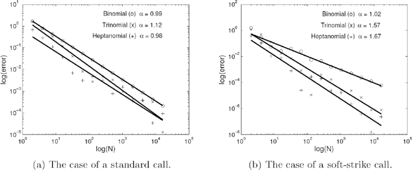
Convergence of multinomial approximations to the Black–Scholes prices of European call options.
(Soft-Strike Call Option under GBM). Power options differ from vanilla European options in that the payoff function is not linear but raised to some power function. In a previous chapter we learned how to analytically price such options under the GBM model. Typically, the terminal payoff of a power option is a quadratic function of the underlying. The widest possible application of power options is for addressing the nonlinear risk of option sellers. There was proposed a class of soft-strike options which do not have a single fixed strike price but a range of strike spread over an interval. Such options allow for addressing limitations of a standard delta hedging when the underlying asset is close to the strike at expiration of the option and any re-balancing of the hedging portfolio causes the underlying asset to become “pinned” to the strike price. Recall that this is related to the fact that the delta position for a standard call approaches a unit step (Heaviside) function as time to maturity goes to zero.
Consider the soft strike European call option with payoff
Λa(S)={0if S<K−a,14a(S−K+a)2if K−a≤S<K+a,S−Kif S>K+a. (18.58)
We have obtained an exact analytical (Black–Scholes) pricing formula for this option in a previous chapter, i.e., see equation (12.45). Note that in the limit as a → 0, the soft-strike payoff converges to the call payoff (S − K)+.
Since the payoff of a soft strike option is a continuously differentiable function of spot, the trinomial and heptanomial model will demonstrate a higher rate of convergence than that of the binomial tree model. Let us compute discrete-time approximations of the exact analytical price of the soft strike call option with K = 100 and a = 5. The other parameters are the same as those of the previous example. By evaluating the standard normal CDF expressions of the analytical pricing formula in (12.45), we obtain the exact option value (within 15 decimals) as 8.351245148287005. Notice that it is slightly larger than the value of a standard European call with the same maturity T and strike K from the previous example. This is expected since the payoff Λa(S) is strictly larger than the call payoff (S − K)+ for K − a < S < K + a. The errors for the multinomial approximations are reported in Table 18.13b and Figure 18.12b. Note that the rate of convergence of the binomial model is linear. The trinomial and heptanomial models demonstrate a superlinear rate of convergence.
18.2.4 Pricing European Options by PDEs
Let us assume the stock price process is a time-homogeneous diffusion with linear drift and local volatility function σ(S), i.e., S(t) satisfies the SDE
dS(t)S(t)=(r−q)dt+σ(S(t))d˜W(t).
A standard European-style derivative has price V = V (t, S) as a function of calendar time t and spot S, where V satisfies the corresponding Black–Scholes PDE
∂V∂t+12σ2(S)S2∂2V∂S2+(r−q)S∂V∂S−rV=0,0≤t≤T,0<S<∞, (18.59)
subject to the terminal (payoff) condition at maturity as t ↗ T :
V(T−,S)≡V(T,S)=Λ(S),0<S<∞, (18.60)
Here, Λ is the payoff function, r and q are, respectively, the risk-free interest rate and dividend rate, the volatility term is a state-dependent function expressed as a product of the spot and local volatility: σ(S)S. Note that this generalizes the case σ(S) = σ, where σ > 0 is the usual constant volatility parameter in the GBM model. Below, we focus on the case of pricing standard (vanilla) European options. The values of European call and put options, denoted below by VC and VP , respectively, satisfy the terminal conditions:
VC(T,S)=(S−K)+≡max {S−K,0}, (18.61)VP(T,S)=(K−S)+≡max {K−S,0}. (18.62)
The Black–Scholes PDE is defined on the domain
D={(t,S)|0≤t≤T,0<S<∞,} (18.63)
which is unbounded as S → ∞. To complete the formulation of the differential problem (18.59)–(18.60), we need to impose a boundary condition on the solution V for S = 0 and an asymptotic condition on V as S → ∞. These conditions depend on the option. For standard European options, we can use the put-call parity and the fact that an option becomes worthless when it is out of the money. The unboundedness of D makes the application of finite-difference numerical schemes unfeasible. One possible solution is to map the semi-infinite interval S ∈ (0, ∞) onto a finite one by applying a suitable change of variables. Another approach is to truncate D to obtain a bounded rectangular domain. Let us introduce a lower bound Smin that represents small asset prices and an upper bound Smax that represents large asset prices. The asset price S is allowed to change in the interval [Smin, Smax]. Consequently, the Black–Scholes PDE is considered in the truncated domain
ˆD={(t,S)|0≤t≤T,Smin ≤S≤Smax }. (18.64)
The selection of Smin and Smax is also dictated by the type of option. For knock-out barrier options we may set Smin = BL and/or Smax = BU , where BL and BU are, respectively, the lower and upper barriers.
We now need to specify the boundary conditions on V at S = Smin and S = Smax. Consider European options for which we set Smin close to zero and Smax very large. A European call option is out of the money (and hence worthless) when S = Smin (as long as Smin≈ 0). Therefore, for the call price VC we adopt the following boundary condition at the left boundary:
VC(t,Smin )=0 for all 0≤t≤T. (18.65)
Similarly, a European put option is out of the money (and hence worthless) when S = Smax (as long as Smax ≫ K). Hence, we set
VP(t,Smax )=0 for all 0≤t≤T. (18.66)
The boundary condition on the other side of ˆD can be obtained by considering the put-call parity
VC(t,S)−VP(t,S)=Se−q(T−t)−Ke−r(T−t) for all 0≤t≤T and S>0. (18.67)
Combining (18.65) and (18.67) at S = Smin gives us the left boundary condition for the put value:
VP(t,Smin )=Ke−r(T−t)−Smin e−q(T−t) for all 0≤t≤T. (18.68)
Combining (18.66) and (18.67) at S = Smax gives us the right boundary condition for the call value:
VC(t,Smax )=Smax e−q(T−t)−Ke−r(T−t) for all 0≤t≤T. (18.69)
Since the payoff functions of a call and put option are linear in the underlying, we can also use the boundary conditions
∂2∂S2VC(t,Smax )=0 and ∂2∂S2VP(t,Smin )=0. (18.70)
18.2.4.1 Pricing by the Heat Equation
As we already saw, the Black–Scholes PDE (18.59) with constant volatility σ reduces to the classical heat equation (18.8) in the spatial variable x and time to maturity τ,
∂u(T,x)∂T=∂2u(T,x)∂x2,
upon applying the following transformation to Equation (18.59):
S=Kex, t=T−τσ2/2,V(t,S)=K e−γx−(β2+ℓ)Tu(τ,x), (18.71)
where the constants γ, β, and l are defined as follows:
γ=12(k−1),β=12(k+1)ℓ=qσ2/2,k=r−qσ2/2. (18.72)
The change of variable in (18.71) maps the original domain D, defined in (18.63), and the truncated domain ˆD, defined in (18.64), to
Du={(τ,x)|0≤τ≤σ22T,−∞<x<∞}, (18.73)ˆDu={(τ,x)|0≤τ≤σ22T,xmin ≤x≤xmax }, (18.74)
respectively, where xmin :=ln (Smin K) and xmax :=ln (Smax K). The terminal conditions (18.61) and (18.62) are transformed into the initial conditions
uC(0,x)=max {eβx−eγx,0}(for the call option), (18.75)uP(0,x)=max {eγx−eβx,0}(for the put option), (18.76)
respectively, for all x ∈ [xmin, xmax]. Finally, the boundary conditions for the heat equation on the truncated domain ˆDu are as follows:
{uC(τ,xmin )=0,uC(τ,xmax )=eβxmax +β2τ−eγxmax +γ2τ(for the call option), (18.77){uC(τ,xmin )=eγxmin +γ2τ−eβxmin +β2τ,uP(τ,xmax )=0(for the put option), (18.78)
for all τ∈[0,σ22T]. To find the numerical solution, we apply one of the finite-difference schemes to the initial boundary value problem obtained.
18.2.4.2 Pricing by the Black–Scholes PDE
Before we introduce a mesh in the domain ˆD and discretize the PDE (18.59), let us rewrite the terminal value problem (18.59)–(18.60) as an initial value problem. We replace the actual time t by the time to maturity τ = T − t in Equations (18.59), (18.60), (18.68), and (18.69) to obtain the following differential equation:
∂υ∂T=12σ2(S)S2∂2υ∂S2+(r−q)S∂υ∂S−rυ,T>0,Smin <S<Smax (18.79)
subject to the initial condition
and the boundary conditions
and
for the European put and call options, respectively. Here, the option value v = v(τ, S) is a function of the spot price S and the time to maturity τ.
Consider a uniform spacial mesh on the interval [Smin, Smax]:
Replacing all derivatives with respect to S by their central finite-difference approximations, we obtain the following approximation to the Black–Scholes PDE (18.79):
Let Vj(τ) denote the semi-discrete approximation to v(τ, sj). Applying (18.83) at each internal node sj, we obtain the following system of first-order ordinary differential equations:
System (18.84) has n equations in n+2 unknown functions V0(τ),V1(τ),...,Vn(τ),Vn+1(τ). Using the boundary conditions we have the functions V0(τ)and Vn+1(τ), which, respectively, approximate the solution at the boundary nodes s0 = Smin and sn+1 = Smax. As a result, the system of differential equations (18.84) can be written as the following matrix-vector differential equation with an n-by-n tridiagonal coefficient matrix L whose entries are defined in (18.84):
subject to the initial condition
Here we use the notation:
The vector G(T) ∈ ℝn is given by
G(τ) contains boundary values of the mesh solution. For vanilla European options we can use the boundary conditions (18.81) and (18.82) to obtain the following:
and
Applying finite differences in time, we derive the explicit method, the implicit method, and the Crank–Nicolson method as follows, by introducing the fully discretized approximate solution (the mesh solution) to the Black–Scholes equation:
The approximation solution at the ith time level will be denoted by
for each i = 0, 1, 2,..., m.
The Explicit Method
Using a forward finite difference in (18.85) gives
which leads to the iterative rule
The Implicit Method
Approximating the time derivative in (18.85) with a backward finite difference gives
which leads to the iterative rule
The Crank–Nicolson Method
The Crank–Nicolson method is derived by taking the arithmetic average of the explicit (18.90) and the implicit (18.90) methods to give the following:
All the above schemes are subject to the initial condition
with Λ defined in (18.86).
In this example we apply the implicit and Crank–Nicolson schemes to price a standard call option under the Black–Scholes (log-normal) model. The parameters used are the same as those of Example 18.9. The truncated domain has the lower bound Smin = 0 and the upper bound
To discretize the PDE problem, we split the space and time intervals in 5001 and 1001 subintervals, respectively. Thus, the time and space discretization steps are
The results for the two schemes are reported in Figure 18.14a. As is seen from the graphs in Figure18.14b, the rate of convergence of the Crank–Nicolson method is higher than that of the implicit method.
18.2.5 Calibration of Asset Price Models to Empirical Data
The term calibration refers to the computational process of fitting an asset price model to historical financial data. First, we select an asset price price model that seems to explain well empirical observations. There are two typical calibration procedures. The least squares method (LSM) allows for fitting model derivative values to the respective market prices. To apply this method, we assume that a derivative pricing formula is available in closed form or that the prices can be computed numerically in a fast and efficient manner. The maximum likelihood estimation (MLE) method allows for fitting the probability distribution to historical asset prices (or their returns). To apply it we assume that a transition probability density is known in closed form. Suppose the model can be characterized by a vector of parameters, say ξ = (ξ 1,ξ 2,...,ξ k). The objective is find the best-fitted vector that solves the respective optimization problem. Typically, there are two levels of calibration: first, an initial full calibration of all parameters of the model and, second, a faster re-calibration conditional on the vector computed previously that can be used as soon as new data have arrived. The second calibration scheme may be used throughout the day or even for longer periods, while the full calibration only needs to be executed at the outset or if markets move considerably.

Computing Black–Scholes call option values with the use of the implicit and Crank–Nicolson methods.
18.2.5.1 Least Squares Method
Suppose we wish to calibrate an asset price model to historical European call and put option prices. Let the option with strike Ki and maturity Ti have an observed price Oi. Thus, we have two arrays of observations, i.e., a pair of variables (Ki,Ti) specifying the option and market prices Oi, where i = 1, 2,..., m. Let the model produce a price Ci = C(Ki,Ti; ξ ) for the same ith option. The goal of the calibration process is to minimize the least squares error between the model and market prices for the m option values:
where wi is a weight that reflects the relative significance of reproducing the ith option price precisely. The suitable choice of the weights wi, i = 1, 2,..., m, is important for good calibration results. The simplest choice is to set . The confidence in individual data points is determined by the liquidity of the option. Thus, the weights can also be evaluated from the bid-ask spreads:
Alternatively, as suggested by Cont and Tankov (2003), one may use the Black–Scholes (BS) “Vegas” evaluated at the implied volatilities of the market option prices to compute the weights:
where ∂CBS/∂σ denotes the derivative of the BS option pricing formula with respect to the volatility σ, evaluated at , and is the BS implied volatility for the observed market price Oi. For the observed market prices Oi we may also use the midpoint of the bid and ask prices, i.e., .
18.2.5.2 Maximum Likelihood Estimation
Suppose the asset price process {S(t)}t≽0 is a Markov process with a transition PDF pξ (u, t; S, S′). The PDF depends on the vector of parameters ξ . Typically, empirical data are available to us in the form of a truncated series of historical asset prices. Consider the array of observations (ti, ŝi), i = 0, 1, 2,..., m, where ŝi is a market asset (stock) price at calendar time ti. In general, the MLE method selects values of the model parameters that produce a probability distribution that gives the observed data the greatest probability. To use the method of maximum likelihood, we first need to specify the joint density function for all observations. Let the times ti form an increasing sequence. The joint probability density of the model asset prices at S(t0) = s0,S(t1) = s1,...,S(tm) = sm is then simply a product of transition PDFs
Now, by substituting the time series of observed asset prices s0 = ŝ0, s1 = ŝ1,..., sm = ŝm, we obtain the likelihood function
The method of maximum likelihood estimates the best-fitted by finding a value of ξ that maximizes L(ξ):
In practice it is often more convenient to work with the (natural) logarithm of the likelihood function, called the log-likelihood. The result is the same regardless of whether we maximize the likelihood or the log-likelihood function, since the natural logarithm is a monotonically increasing function.
In solving the problems (18.92) and (18.93), we apply a numerical optimization routine such as the Nelder–Mead method (a nongradient based algorithm) or gradient search methods. In practice, the parameters ξ 1,ξ 2,...,ξ k have lower and/or upper constraints. However, by changing variables, a constrained optimization problem can be transformed into one without constrains.
18.3 Pricing Early-Exercise and Path-Dependent Options
Pricing exotic derivatives such as American and Asian options is a much less trivial problem in comparison to pricing standard European options. There are no closed-form formulae for the American and the arithmetic Asian options within the Black–Scholes model. In this section we focus on pricing options with an underlying asset price following the log-normal model or another Markov process whose transition distribution is known in closed form.
18.3.1 Pricing American and Bermudan Options
18.3.1.1 Pricing American Options by Tree Methods
Consider the application of the binomial tree method to pricing an American option with time to maturity T > 0 and having the intrinsic payoff value Λ(S). The continuous-time asset price process, which follows the log-normal model, is approximated by a discrete-time binomial model with N + 1 trading dates {n δt : n = 0, 1,...,N}, where δt is the length of one period and N δt = T . Let the factors u and d be specified as in (18.46). The one-period interest rate is erδt − 1. The risk-neutral probability of the upward move is given in (18.47).
Let Vn, k denote the American option value at time n δt for the asset price Sn, k = S0undn − k with k = 0, 1,..., n and n = 0, 1,...,N. From Chapter 7, we know that a backward-in-time recursion relation can be used to compute the option value at each node of the binomial tree as follows.
1. At maturity, set VN, k = Λ(SN, k) for each k = 0, 1,...,N.
2. For each n = N − 1,N − 2,..., 0 and k = 0, 1,..., n, the option value Vn, k is given by
Let us see how the above algorithm can be used to compute prices of a Bermudan derivative that can only be exercised at discrete times 0 < t1 < t2 <··· < tM = T with M ≪ N. Assume that the exercise dates are all of the form n δt for some integer n. At each exercise date, the option value is a maximum of the continuation and the intrinsic values. In between the exercise dates, we treat the derivative as a European option. The steps are as follows.
1. At maturity, set VN, k = Λ(SN, k) for each k = 0, 1,...,N.
2. For each n = N − 1,N − 2,..., 0, compute the option values Vn, k, k = 0, 1,..., n, as follows:
(i) Compute the continuation values
(ii) If n δt is an exercise date, i.e., n δt = tm for some m = 1, 2,...,M, then
otherwise, we set
In this example, we compute discrete-time approximations for the Black–Scholes price of American and Bermudan put options with T = 1, K = 95, S0 = 100, r = 0.05, q = 0, and σ = 0.25. As for the Bermudan options, we assume that the option can only be exercised at one of the M times , m = 1, 2,...,M. The results of our calculations are reported in Tables 18.15a and 18.15b.
18.3.1.2 Pricing Bermudan Options by the Monte Carlo Method
Instead of a continuously exercisable American option, we consider a Bermudan option that can only be exercised at a fixed set of times 0 < t1 < t2 <··· < tM = T . The option expires at time T and the payoff to the holder is Λ(S). The American option can be viewed as a limiting case of Bermudan options as M→ ∞ and max1≼k≼M|tk − tk − 1 | → 0. Suppose that the number M of exercise times is not too large. Even in this case the early-exercise option price problem poses a significant challenge to the Monte Carlo method.
Pricing options in the binomial tree model.
N |
δt |
European |
American |
M |
Bermudan |
|
|---|---|---|---|---|---|---|
100 |
0.01 |
5.3957684 |
5.7494428 |
2 |
5.5609302 |
|
200 |
0.005 |
5.4240877 |
5.7388323 |
5 |
5.6629469 |
|
500 |
0.002 |
5.4165327 |
5.7584385 |
10 |
5.7042806 |
|
1000 |
0.001 |
5.4147939 |
5.7517360 |
20 |
5.7262399 |
|
2000 |
0.0005 |
5.4148298 |
5.7502178 |
50 |
5.7400010 |
|
5000 |
0.0002 |
5.4140541 |
5.7501685 |
5000 |
5.7501685 |
|
(a) Pricing European and American puts with N periods. |
(b) Pricing Bermudan puts with N = 5000 periods and M exercise dates. |
|||||
The initial price of a Bermudan option can be calculated using a backward-in-time recursion. Let V (t, S) denote the no-arbitrage price at time t given that S(t) = S and the option has not been exercised before time t. It is more convenient to write the equation on the option values using discounted quantities. Consider the discounted payoff function Λk(S) = e−rtk Λ(S) at the exercise time tk. Let Vk(S) denote the present value of the time-tk option price. That is, Vk(S) = e−rtk V (tk,S) is the no-arbitrage option value calculated at time tk and discounted to time 0. We also denote Sk = S(tk) for all k = 0, 1,...,M. At the maturity time T = tM we have VM (S) = ΛM (S). At any exercise time tk < tM the holder of the option can exercise the option and immediately receive the payoff (the intrinsic value), or continue to hold the option. In the latter case, the average proceeds to the holder are given by the expected time-tk+1 option value (the continuation value). Therefore, the discounted option values Vk satisfy the following dynamic programming problem:
The mathematical expectations considered here are computed under the risk-neutral probability measure :
The main difficulty of the problem is the computation of the continuation value. Let us consider three Monte Carlo approaches to dealing with this issue. Note that the asset price process {S(t)}t≽0 does not necessarily follow geometric Brownian motion. The only assumption regarding the underlying asset process we will require is that the Markov chain S0→ S1→ S2→ ···→ SM can be simulated exactly from the transition probability distribution. Although we only discuss the single-asset case, all the methods presented below can also be used for the evaluation of multi-asset Bermudan options.
Stochastic Tree Method. For each tk, the continuation value can be approximated by the Monte Carlo method. First, sample b successors from the exact probability distribution of Sk+1 conditional on Sk. Second, approximate the mathematical expectation by the sample mean:
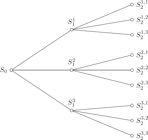
The main idea of the stochastic tree method is to construct a nonrecombining stochastic tree with M levels (so that each level corresponds to one of M exercise times) and b branches for each node. As a result we obtain a tree with bM branches at the last level (see Figure 18.16). Since the number of branches grows exponentially fast as M increases, this method is feasible only if both b and M are not very large. Algorithm 18.3 describes the construction of a stochastic tree in detail.
Stochastic Mesh Method. The main shortcoming of the stochastic tree method is that the number of branches of a stochastic tree grows exponentially-fast as the number M of exercise times increases. The stochastic mesh method proposed by Broadie and Glasserman (2004) also operates with a random tree, but there are two key distinctions. First, there is no branching at intermediate times and the total number of sample paths does not explicitly depend on the number of exercise times. We start with sampling n paths of the Markov chain S0→ S1→ S2→ ···→ SM , where Sk≡ S(tk) for all k. These paths form a stochastic tree with n branches (and n· M nodes) all originated at time 0. Second, in computing the continuation value at some time tk we use time-tk+1 option values from all branches regardless of whether or not the values are computed for the successor of the current node. Algorithm 18.4 describes the stochastic mesh method step by step. In comparison with the stochastic tree method, we additionally assume that the risk-neutral transition PDF (under the risk-neutral measure) is known in closed form. Note that, for simplicity, we are assuming a time-homogeneous process.
To explain the formula for the weights, let us consider the computation of the continuation value in more detail. In computing the Monte Carlo approximation of the continuation value , the asset values at time tk+1 are not sampled from the single time-step transition PDF . Since all paths begin with S0, the values at time tk+1 are sampled from the marginal PDF (tk+1; S0,S). At the node (tk,) we have
(multiply and divide the integrand by p(tk+1; S0,S))
where the time-tk+1 asset price Sk+1 has probability density in the last mathematical expectation. As we can see, in computing the option value at the node (tk,) we use the option values from all nodes at the next time layer tk+1, as is illustrated in Figure 18.17, which gives a complete picture of all relations between the nodes of the stochastic tree. The tree looks more like a net or mesh. This structure explains the name of the stochastic mesh method.
Algorithm 18.3 The Stochastic Tree Method for Estimation of the No-Arbitrage Value of a Bermudan Option.
- (1) Starting from the initial asset price value S0 we simulate b independent successors all having the probability law of S1≡ S(t1).
- (2) For each , simulate b independent successors
all having the law of S2≡ S(t2) conditional on .
- (3) For each , i1, i2 = 1, 2,..., b, simulate b independent successors
all having the law of S3≡ S(t3) conditional on .
⋮
- (M) For each =1,2,..., b, simulate b independent successors
all having the law of SM≡ S(tM) conditional on .
Let denote the approximation of the option value at time tk for the asset price . At the terminal nodes we set the option value equal to the payoff value:
Working backward in time throughout the tree, we can compute option values for each node of the tree. Starting with k = M − 1, for each k = M − 1,M − 2,..., 1, we set
Finally, we calculate the approximation of the option price at current time t = 0 by

Construction of stochastic mesh from independent paths. The figure on the left shows the nodes and the figure on the right contains all the paths up to three time steps.
Theorem 18.4
(Broadie and Glasserman (2004)). The mesh estimator 0 is biased high, i.e., E[0] ≽ V (0,S0) for all n ≽ 1.
Proof. Let us prove the assertion by using Jensen’s inequality and induction. At the terminal time tM = T we have for all i = 1, 2,..., n. Assume for some k = 0, 1,...,M − 1 and all i = 1, 2,..., n. At time tk we have
Algorithm 18.4 The Stochastic Mesh Method for Estimation of the No-Arbitrage Price of a Bermudan Option.
- Generate n independent paths using the transition PDF p. That is, is sampled from the density for every k = 1, 2,...,M and every j = 1, 2,..., n. Here all equal S0. The sample paths form a stochastic tree starting at S0 with n· M nodes. The node (k, j) corresponds to the exercise time tk and asset price .
- At the terminal nodes (corresponding to the time tM≡ T), we set
- Working recursively backward in time, we set
for k = M − 1,M − 2,..., 1 and i = 1, 2,..., n. Here are weights given by
- Calculate the approximation of the initial option value, .
In conclusion, we mention another popular Monte Carlo technique for pricing Bermudan options based on the least squares (regression) method by Longstaff and Schwartz (2001). Regression methods rely on the representation of the continuation value as a linear combination of some basis functions ψℓ : ℝ→ ℝ, ℓ = 1, 2,...,L. That is, the single time-step conditional expectation is written as a linear combination of a chosen set of so-called basis functions:
18.3.2 Pricing Asian Options
Asian options are averaging options, where the payoff functions depend on some form of average of the underlying asset prices over the life of the option. By considering different types of averaging, such as arithmetic or geometric, continuous or discrete, one can obtain different types of options. The difficulty with the pricing of Asian options depends both on the underlying asset price model and on the type of the option. If we assume the asset price follows the GBM process, then one can derive closed-form pricing formulae for Asian options with geometric averaging. Pricing arithmetic Asian options is a computational challenge even under the GBM model.
18.3.2.1 Pricing Discrete-Time Asian Options by the Monte Carlo Method
Here we analyze only one type of averaging, namely, discrete arithmetic averaging at M time observation points equally spaced throughout [0,T], with random variables
By using methods of extrapolation, one can also approximate values of Asian options for continuous-time arithmetic averaging based on option values computed using discrete averaging. Most Asian options are of European style (i.e., not early exercise). There are two main examples of Asian options: the arithmetic average price (AAP) or floating price option and the arithmetic average strike (AAS) or floating strike option. The payoff functions of Asian calls (C) and puts (P) with time to maturity T are as follows:
The plain Monte Carlo evaluation of the no-arbitrage price of an Asian option with a payoff function of the form Λ(AM ,SM) is straightforward.
- Generate n independent sample paths , j = 1, 2,..., n, all starting at the initial spot S0.
- For each path, calculate the arithmetic average
- The no-arbitrage price of the option is approximated by the discounted sample mean of the payoff values
- Additionally, we can estimate the variance
to construct an asymptotically valid 100(1 − α)% confidence interval for V0:
To implement the above algorithm, we only assume that sample paths can be generated exactly or approximately with high accuracy. Though the plain Monte Carlo approach is easy to implement, it is not very efficient. Several variance reduction methods have been proposed for valuing derivatives. In Boyle et al. (1997), the performances of the antithetic variate method, control variate (CV) method, and moment matching method were compared to that of the direct Monte Carlo method. They showed by simulation that the control variate method is the most efficient for valuing an Asian option. The CV method, considered in Boyle et al. (1997), was used to improve upon a naive Monte Carlo estimator for an Asian call option by choosing as analytical control variate the corresponding Asian call option with geometric averaging. We focus on this method of variance reduction.
We can achieve a larger variance reduction by considering multiple control variates. Suppose that there are two random variables Y (1) and Y (2) with respective means ν1 and ν2 known analytically. We construct the controlled Monte Carlo estimator of the mean of a random variable X, E[X] = μ, by using the random variable defined by
For all values of the parameters c1 and c2, the mean of Z coincides with the mean of X. The variance of the controlled estimator Z is
where
The optimal values of c1 and c2 that minimize Var(Z) can be found by solving simultaneous linear equations for i = 1, 2:
The solution to (18.100) is the optimal vector
Substituting it back into (18.99) gives
Here the ratio measures the strength of the linear relation between X and Y. It generalizes Corr2(X, Y) for X and scalar Y . As in the scalar case, the optimal vector of coefficients copt can be estimated by using sample estimates:
where the (i, k)th entry of the square matrix SY,Y is
and the ith entry of the column vector SX,Y is
where (Xj,Y (1)j,Y (2)j), j = 1, 2,..., n are i.i.d. samples, and and (i) are sample means given by
respectively.
Let us consider the arithmetic average price call option with the payoff given by (18.97) within the GBM model. The variance of the naive Monte Carlo estimator can be significantly reduced with the use of multiple control variates. One control variate is the geometric Asian option, which can be evaluated analytically. The other control variate is an option whose payoff is an average of European payoffs with different maturity times. Let us find out how the payoffs of these control variates relate to the payoff of the average price call. According to the inequality of arithmetic and geometric means, the arithmetic mean of a set of nonnegative real numbers is greater than or equal to the geometric mean of the same set. That is,
Using this and the fact that max{x, 0} is increasing in x, we have a lower bound for the payoff function:
If the asset price {S(t)}t≽0 follows GBM, then GM is log-normally distributed and hence the geometric option with payoff max{GM − K, 0} can be priced analytically. Let denote the no-arbitrage time-0 value of the geometric average price call with the payoff .
Since (x)+≡ max{x, 0} is a convex function of x, we have the following upper bound for :
which leads us to consider a new option with the payoff
as a control variate for the average price call. As is readily observed, the payoff is just an average of European call payoff functions at exercise times tk, k = 1, 2,...,M. The price can be computed numerically using only univariate integrals:
As a result, we can improve the plain Monte Carlo algorithm, as follows.
- Generate n independent sample paths , all starting at spot S0.
- For each path, labelled j = 1, 2,..., n, calculate
- (a) the arithmetic average ,
- (b) the geometric average ,
- (c) the arithmetic average price payoff ,
- (d) the geometric average price payoff ,
- (e) the arithmetic average of European call payoffs .
- Estimate the optimal coefficients c1 and c2: , with the respective 2-by-2 matrix and 2-by-1 vector:
- Calculate the sample values of the controlled estimator
where and .
- The approximate no-arbitrage price of the AAP call option is then:
- Estimate the variance
and construct the confidence interval for :
with an asymptotically valid 100(1 − α)% confidence level.
Pricing an arithmetic average price call option using control variate Monte Carlo methods.
Control |
Estimate |
Error |
Speedup |
|---|---|---|---|
None |
6.050039 |
0.037420 |
|
AAC |
6.052996 |
0.003871 |
93.45 |
GAP |
6.051365 |
0.001051 |
1266.68 |
GAP+AAC |
6.051600 |
0.000845 |
1961.39 |
Let us study the efficiency of the single and multiple control variate methods for Monte Carlo pricing of an AAP Asian call option. The underlying asset price follows the geometric Brownian motion model with σ = 0.25, r = 0.05, q = 0, T = 1. The spot value and strike price are, respectively, S0 = 100 and K = 100. The number of observation time moments is M = 128. Using the Black–Scholes pricing formula, we first compute the expected values of the control variates:
After that, the Asian call option price is estimated by the Monte Carlo method using n = 10,000 sample paths. In Table 18.18 we report the simulation results for the crude estimate and three control variate estimates using, respectively, the geometric average price call (GAP), arithmetic average of European calls (AAC), and both averages as controls. The control variate method is very efficient. This observation is also supported by high correlation between the crude estimate and the GAP/AAC control estimates. The respective correlations coefficients are
References
J. Alford and N. Webber. Very high order lattice methods for one factor models. Available at SSRN 259478, 2001.
P. Boyle, M. Broadie, and P. Glasserman. Monte Carlo methods for security pricing. Journal of Economic Dynamics and Control, 21(8):1267–1321, 1997.
M. Broadie and P. Glasserman. A stochastic mesh method for pricing high-dimensional American options. Journal of Computational Finance, 7:35–72, 2004.
R. Cont and P. Tankov. Financial Modelling with Jump Processes. Chapman & Hall/CRC, 2003.
S. Heston and G. Zhou. On the rate of convergence of discrete-time contingent claims. Mathematical Finance, 10(1):53–75, 2000.
F. A. Longstaff and E. S. Schwartz. Valuing American options by simulation: A simple least-squares approach. Review of Financial Studies, 14(1):113–147, 2001.
D. B. Madan, P. Carr, and E. C. Chang. The Variance Gamma process and option pricing. European Finance Review, 2(1):79–105, 1998.
1Recall that the eigenvalues are zeros of the polynomial det(A − λIn).