Chapter 10

One-Dimensional Brownian Motion and Related Processes

Brownian motion is a keystone in the foundation of mathematical finance. Brownian motion is a continuous-time stochastic process but it can be constructed as a limiting case of symmetric random walks. Recall that a similar approach was used to obtain the log-normal price model as a limiting case of binomial models. Since the probability distribution of Brownian motion is normal, it is reasonable to begin with reviewing some of the important basic facts about the multivariate normal distribution.

10.1 Multivariate Normal Distributions

10.1.1 Multivariate Normal Distribution

The n-variate normal distribution is determined by an n × 1 mean vector μ and an n × n positive definite covariance matrix C = C⊤:

$\mu ={\left[{\mu }_1,{\mu }_2,...,{\mu }_n\right]}^{⊺},C={\left[C_{ij}\right]}_{i,j=1,...,n}.$

Note: throughout we use superscript ⊤ to denote the transpose. We denote the n-variate normal distribution with mean vector μ and covariance matrix C by Normn(μ, C). Assuming the nondegenerate case with a positive definite covariance matrix, the joint probability density function (PDF) is an n-variate real-valued function

$f\left(\text{x}\right)=\frac{1}{{\left(2\pi \right)}^{n/2}{\left[\det C\right]}^{n/2}}{\text{e}}^{-\frac{1}{2}{\left(\text{x}-\mu \right)}^{⊺}{C}^{-1}\left(\text{x}-\mu \right)},\text{x}\in {ℝ}^n.\text{ (10.1)}$

This PDF is that of random vector X = [X1,X2,...,Xn]⊤ ~ Normn(μ, C), i.e., X has n-variate normal distribution with mean μ = E[X] and covariance C = E[XX⊤] − μμ⊤. As components, μi = E[Xi] and Cij = Cov(Xi,Xj) = E[XiXj] − μiμj, i, j = 1, 2 ...,n. It is a well-known fact that normal random variables are independent iff they are uncorrelated with zero covariances Cij = 0 for all i ≠ j. Therefore, if the covariance is a diagonal matrix, $C=\text{diag}\left({\sigma }_1^2,{\sigma }_2^2,...,{\sigma }_n^2\right)$, where ${\sigma }_i^2=\text{E}\left[{\left(X_i-{\mu }_i\right)}^2\right]$, then the components of X are (mutually) independent normally distributed random variables. In this case, the joint PDF is a product of one-dimensional marginal densities:

$f\left(\text{x}\right)={\displaystyle \prod _{i=1}^n\frac{1}{{\sigma }_i}n\left(\frac{x_1-{\mu }_i}{{\sigma }_i}\right)}={\displaystyle \prod _{i=1}^n\frac{1}{\sqrt{2\pi }{\sigma }_i}{\text{e}}^{-\frac{{\left(x_i-{\mu }_i\right)}^2}{2{\sigma }_i^2}}}.$

Here we used the notation $n\left(z\right)={\mathcal{N}}^{\prime }\left(z\right)=\frac{{\text{e}}^{-z^2/2}}{\sqrt{2\pi }}$ for the PDF of the standard normal. Another well-known fact is that a sum of normal random variables is again normally distributed:

$X_i~Norm\left({\mu }_i,{\sigma }_i^2\right),i=1,2\Rightarrow X_1+X_2~Norm\left({\mu }_1+{\mu }_2,\text{Var}\left(X_1+X_2\right)\right),\text{ (10.2)}$

where Var (X1 + X2)= σ12 + 2 Cov(X1,X2)+ σ22. This property extends to the multivariate case as follows. Let a and B be an m × 1 constant vector and an m × n constant matrix, respectively, with 1 ≤ m ≤ n. Suppose that X ~ Normn(μ, C); then the m-variate random vector a + BX is normally distributed with mean vector a + B μ. Its covariance matrix is given by E[B(X − μ)(B(X − μ))⊤]= B E[(X − μ)(X − μ)⊤] B⊤ = BCB⊤. Hence, provided that det(BCB⊤) ≠ 0, we have:

$X~Nor{m}_n\left(\mu ,C\right)\Rightarrow \text{a}+BX~Nor{m}_m\left(\text{a}+B\mu ,BC{B}^{⊺}\right),\text{ (10.3)}$

This property allows us to express an arbitrary multivariate normal vector in terms of independent standard normal variables. Since the covariance matrix C is positive definite, it admits the Cholesky factorization: C = LL⊤ with a lower-triangular n × n matrix L. Let Z11,Z2,...,Zn be i.i.d. standard normals. The vector Z = [Z1,Z2,...,Zn]⊤ is then an n-variate normal with mean vector zero and having the identity covariance matrix I. Applying (10.3) to Z ~ Normn(0, I) gives μ + LZ ~ Normn(μ, C), i.e., in this case the vector μ + LZ has mean μ + L0 = μ and covariance matrix LIL⊤ = LL⊤ = C.

10.1.2 Conditional Normal Distributions

Suppose that X = [X1,X2,...,Xn]⊤ ~ Normn(μ, C), n ≥ 2. Let us split (partition) the vector X into two parts:

$X=\left[\begin{array}{c}{X}_1\\ X_2\end{array}\right],\text{where}{X}_1\in {ℝ}^m\text{and}{X}_2\in {ℝ}^{n-m}$

for some m with 1 < m < n. Correspondingly, we split the vector μ and matrix C to represent them in a block form:

$\mu =\left[\begin{array}{c}{\mu }_1\\ {\mu }_2\end{array}\right]\text{and}C\text{=}\left[\begin{array}{cc}{C}_{11}& C_{12}\\ C_{21}& C_{22}\end{array}\right],$

where μ1 ∊ ℝm and μ2 ∊ ℝn−m are the respective mean vectors of X1 and X2; C11 = E[X1X1⊤] is m × m, C12 = E[X1X2⊤] is m × (n − m), C21 = C12⊤ is (n − m) × m, and C22 = E[X2X2⊤] is (n − m) × (n − m). Then, the conditional distribution of X1 given the value of X2 = x2 is normal:

$X_1|\left\{X_2={\text{x}}_2\right\}~Nor{m}_m\left({\mu }_1+C_{12}{C}_{22}^{-1}\left({\text{x}}_{\text{2}}-{\mu }_2\right),C_{11}-C_{12}{C}_{22}^{-1}{C}_{21}\right).\text{ (10.4)}$

For example, consider a two-dimensional (bivariate) normal random vector

$X=\left[\begin{array}{c}{X}_1\\ X_2\end{array}\right]~Nor{m}_2\left(\left[\begin{array}{c}{\mu }_1\\ {\mu }_2\end{array}\right],\left[\begin{array}{cc}{\sigma }_1^2& \rho {\sigma }_1{\sigma }_2\\ \rho {\sigma }_1{\sigma }_2& {\sigma }_2^2\end{array}\right]\right).$

In conformity with (10.4), X1 conditional on X2 (and vice versa) is normally distributed. In this case, m = n − m = 1 so the block matrices are simply numbers: C11 = σ12, C12 = C21 = ρσ1σ2, C22 = σ22, and x2 − μ2 = x2 − μ2. In particular,

$X_1|\left\{X_2=x_2\right\}~Norm\left({\mu }_1+\rho \frac{{\sigma }_1}{{\sigma }_2}\left(x_2-{\mu }_2\right),{\sigma }_1^2\left(1-{\rho }^2\right)\right).\text{ (10.5)}$

10.2 Standard Brownian Motion

10.2.1 One-Dimensional Symmetric Random Walk

Consider the binomial sample space Ω ≡ Ω∞:

${\Omega }_{\infty }={\displaystyle \prod _{i=1}^{\infty }\left\{D,U\right\}}=\left\{{\omega }_1{\omega }_2...|{\omega }_i\in \left\{D,U\right\},\text{for}\text{all}i\ge 1\right\}$

generated by a Bernoulli experiment using any number of repeated up or down moves. We assume a probability measure ℙ such that the up and down moves are equally probable. That is, each outcome ω = ω1ω2 ... ∊ Ω∞ is a sequence of U’s and D’s where $\mathbb{P}\left({\omega }_i=\text{D}\right)=\mathbb{P}\left({\omega }_i=\text{U}\right)=\frac{1}{2}$ for all i ≥ 1. We note that, in contrast to the binomial model where we had a finite number of moves N ≥ 1 with Ω = ΩN, the number of moves is now infinite and the sample space Ω∞ is uncountable. Nevertheless, the discrete-valued random variables that were previously defined on ΩN (e.g., Un, Dn, Bn, etc.) are still defined in the same way on Ω∞. The sample space now also admits uncountable partitions. Obviously, we still have all the countable partitions in the same manner as we discussed for ΩN. For example, the event that the first move is up is the atom AU = {ω1 = U} = {Uω2ω3 ... | ωi ∊{D, U}, for all i ≥ 2}and its complement is AD = {ω1 = D} = {Dω2ω3 ... | ωi ∊{D, U}, for all i ≥ 2} where Ω∞ = AU ∪ AD. In particular, the atoms that correspond to fixing (resolving) the first n ≥ 1 moves are given similarly,

$A_{{\omega }_1^{*}...{\omega }_n^{*}}:=\left\{{\omega }_1={\omega }_1^{*},...,{\omega }_n={\omega }_n^{*}\right\}=\left\{{\omega }_1^{*}...{\omega }_n^{*}{\omega }_{n+1}...|{\omega }_i\in \left\{D,U\right\},i\ge n+1\right\}.$

The union of these 2n atoms is a partition of Ω∞, for every choice of n ≥ 1. We denote by ℱ∞ the σ-algebra generated by all the above atoms corresponding to any number of moves n ≥ 1. Recall that for every N ≥ 1, {ℱn}1≤n≤N is the natural filtration generated by the moves up to time N. We saw that the natural filtration can be equivalently generated by any of the above sets of random variables that contain the information on all the moves, i.e., ℱ0 = {∅, Ω}, ℱN = σ(ω1,...,ωN)= σ(M1,...,MN)= σ({Uk :1 ≤ n ≤ N}), etc. For every N, {ℱn}1≤n≤N is the natural filtration for the binomial model up to time N, where ℱn ⊂ ℱn+1 for all n ≥ 0. In the limiting case of N →∞ we have ${ℱ}_{\infty }={\cup }_{n=1}^{\infty }{ℱ}_n$, or equivalently: ${ℱ}_{\infty }=\sigma \left(\left\{{\omega }_n:n\ge 1\right\}\right)=\sigma \left(\left\{M_n:n\ge 1\right\}\right)=\sigma \left(\left\{{\cup }_n:n\ge 1\right\}\right)$. Hence, ℱ∞ contains all the possible events in the binomial model with infinite moves for which we can compute probabilities of occurrence. For every given N ≥ 1, (ΩN, ℱN, ℙ) is a probability space on which we can define any random variable that may depend on up to N numbers of moves (i.e., random variables that are ℱn-measurable for 1 ≤ n ≤ N). Passing to the limiting case, the triplet (Ω∞, ℱ∞, ℙ) is then a probability space for any random variable that depends on any number of moves (i.e., random variables that are ℱn-measurable for all n ≥ 1), i.e., (Ω∞, ℱ∞, ℙ, {ℱn}n≥1) is a filtered probability space.

Recall that the symmetric random walk {Mn}n≥0 is defined by M0 = 0 and

$M_n\left(\omega \right)={\displaystyle \sum _{k=1}^n{X}_k\left(\omega \right)},\text{where}{X}_k\left(\omega \right)=\{\begin{array}{l}1\text{if}{\omega }_k=U,\hfill \\ -1\text{if}{\omega }_k=D,\hfill \end{array}$

for n, k ≥ 1. Let us summarize the properties of the symmetric random walk.

1. It is a martingale w.r.t. {ℱn}n≥0 and has zero mean, E[Mn] ≡ 0 for all times n ≥ 0.

2. It is a square-integrable process, i.e., E[Mn2] < ∞, such that Var(Mn)= n and Cov(Mn,Mk)= n ∧ k, for n, k ≥ 0.

   Proof. Calculate the variance and covariance of this process as follows:

   $\begin{array}{ll}\text{Var}\left(M_n\right)\hfill & ={\displaystyle \sum _{k=1}^n\text{Var}\left(X_k\right)=n\left(\text{since}{\left\{X_k\right\}}_{k\ge 1}\text{are}\text{i}.\text{i}.\text{d}\text{.}\right),}\hfill \\ \text{Cov}\left(M_{n,}{M}_k\right)\hfill & =\text{E}\left[M_n{M}_k\right]-\underset{=0}{\underbrace{\text{E}\left[M_n\right]\text{E}\left[M_k\right]}}=\text{E}\left[\text{E}\left[M_n{M}_k|{ℱ}_{n\wedge k}\right]\right]\hfill \\ \hfill & =\text{E}\left[\text{E}\left[M_{n\wedge k}{M}_{n\vee k}|{ℱ}_{n\wedge k}\right]\right]=\text{E}\left[M_{n\wedge k}\text{E}\left[M_{n\vee k}|{ℱ}_{n\wedge k}\right]\right]\hfill \\ \hfill & =\text{E}\left[M_{n\wedge k}^2\right]=\text{Var}\left(M_{n\wedge k}\right)=n\wedge k.\hfill \end{array}$

   We note that the above result is also easily proven by using the independence of Mn − Mk and Mk, for n ≥ k.

3. It is a process with independent and stationary increments such that E[Mn − Mk]=0 and Var(Mn − Mk) = |n − k|, for n, k ≥ 0.

Proof. The independence and stationarity of increments are easily proved (as shown in a previous example). The expected value and variance are

$\begin{array}{ll}\text{E}\left[M_n-M_k\right]\hfill & =\text{E}\left[M_n\right]-\text{E}\left[M_k\right]=0-0=0,\hfill \\ \text{Var}\left(M_n-M_k\right)\hfill & =\text{Var}\left(M_n\right)-2\text{Cov}\left(M_{n,}{M}_k\right)+\text{Var}\left(M_k\right)\hfill \\ \hfill & =n-2\left(n\wedge k\right)+k=n\vee k-n\wedge k=|n-k|.\hfill \end{array}$

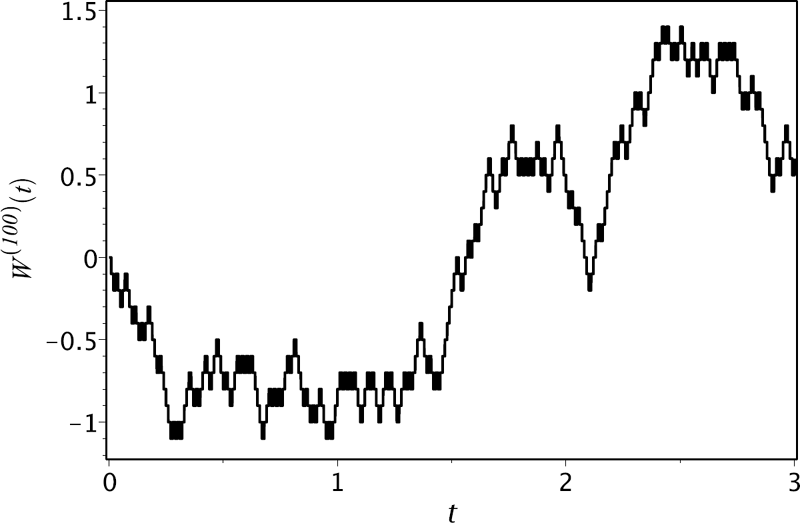
The next step toward Brownian motion (BM) is the construction of a scaled symmetric random walk. We denote this process by W(n) and it will be derived from a symmetric random walk. Fix n ∊ ℕ. For t ≥ 0, define $W^{\left(n\right)}\left(t\right):=\frac{1}{\sqrt{n}}{M}_{nt}$ provided that nt is an integer. Suppose that nt is noninteger. Find s such that ns is an integer and ns < nt > ns +1 holds. Since ns is the largest integer less than or equal to nt, it is equal to $\lfloor nt\rfloor$. We hence define $W^{\left(n\right)}\left(t\right):=W^{\left(n\right)}\left(s\right)=\frac{1}{\sqrt{n}}{M}_{ns}$ to obtain the following general formula of the scaled symmetric random walk:

$W^{\left(n\right)}\left(t\right)=\frac{1}{\sqrt{n}}{M}_{\lfloor nt\rfloor },t\ge 0.\text{ (10.6)}$

As is seen from (10.6), W(n) is a continuous-time stochastic process with piecewise-constant right-continuous sample paths. At every time index $t-\frac{k}{n},k=1,2,...$, the process has a jump of size $\frac{1}{\sqrt{n}}$. Figure 10.1 depicts a sample path of this process for n = 100.

Clearly, the time-t realization W(n)(t) depends on the first $\lfloor nt\rfloor$ up or down moves ω1,...,ωk, with $k=\lfloor nt\rfloor$. Note that since the process W(n) is constant on the time interval, we have $\lfloor nt\rfloor \le nt<\lfloor nt\rfloor +1$. Thus, W(n)(t) is measurable w.r.t. ${ℱ}_{\lfloor nt\rfloor }=\sigma \left(M_1,...,M_{\lfloor nt\rfloor }\right)=\sigma \left(W^{\left(n\right)}\left(u\right):0\le u\le t\right)$. Hence, the filtration defined by ${\mathbb{F}}^{\left(n\right)}:=\left\{{ℱ}^{\left(n\right)}\left(t\right):={ℱ}_{\lfloor nt\rfloor };t\ge 0\right\}$ is in fact the natural filtration for the process {W(n)(t)}t≥0. The process is hence adapted to ${\mathbb{F}}^{\left(n\right)}$. Since the scaled symmetric random walk is obtained by re-scaling (and constant interpolation) of the symmetric random walk, it inherits the properties of the original process. For all t, s ≥ 0 such that ns and nt are integers, we have

1. E [W(n)(t) |ℱ(n)(s)] = W(n)(s) (martingale property) for 0 ≤ s ≤ t, and zero time-t expectation E[W(n)(t)] = 0;

2. Var(W(n)(t)) = t and Cov(W(n)(t),W(n)(s)) = t ∧ s.

3. Let $0\le t_0<t_1<...<t_n$ be such that ntj is an integer for all 0 ≤ j ≤ n, then the increments $W^{\left(n\right)}\left(t_1\right)-W^{\left(n\right)}\left(t_0\right),...,W^{\left(n\right)}\left(t_n\right)-W^{\left(n\right)}\left(t_n-\right)$ are independent and stationary with mean zero and variance $\text{Var}\left(W^{\left(n\right)}\left(t_j\right)-W^{\left(n\right)}\left(t_{j-1}\right)\right)=t_j-t_{j-1}$ for 1 ≤ j ≤ n.

The proof of these properties is left as an exercise for the reader (see Exercise 10.5).

An important characteristic of a stochastic process is the so-called quadratic variation. This quantity is a random variable that characterizes the variability of a stochastic process. For t ≥ 0, the quadratic variation of the scaled random walk W(n) on [0,t], denoted by [W(n),W(n)](t), is calculated as follows on any given path ω ∊ Ω. We go from time 0 to time t along the path, calculating the increments over each time step of size $\frac{1}{n}$. All these increments are then squared and summed up. For t ≥ 0, such that $\lfloor nt\rfloor =nt$ is an integer,

$\begin{array}{ll}\left[W^{\left(n\right)},W^{\left(n\right)}\right]\left(t\right)\hfill & ={\displaystyle \sum _{k=1}^{nt}{\left[W^{\left(n\right)}\left(\frac{k}{n}\right)-W^{\left(n\right)}\left(\frac{k-1}{n}\right)\right]}^2}\hfill \\ \hfill & ={\displaystyle \sum _{k=1}^{nt}{\left[\frac{1}{\sqrt{n}}{X}_k\right]}^2={\displaystyle \sum _{k=1}^{nt}\frac{1}{n}=t\left(\text{since}{X}_k^2=1,1\le k\le n\right).}}\hfill \end{array}\text{ (10.7)}$

The above quadratic variation was calculated to be time t for any path or outcome ω. For every path of the scaled random walk, the quadratic variation [W(n),W(n)](t) is hence a constant and equal to t, i.e., [W(n),W(n)](t)= t is a constant random variable. Recall that the variance of W(n)(t) also has the same value.

The probability distribution of Mm is that of a shifted and scaled binomial random variable: Mm = 2Um − m with Um ~ $Bin\left(m,\frac{1}{2}\right)$. Therefore, the mass probabilities of the scaled random walk are also binomial ones:

$\mathbb{P}\left(W^{\left(n\right)}\left(t\right)=\frac{2k-m}{\sqrt{n}}\right)=\mathbb{P}\left(U_m=k\right)=\frac{m!}{k!\left(m-k\right)!}{\left(\frac{1}{2}\right)}^m,k=0,1,...,m,m=\lfloor nt\rfloor .$

For example, W(100)(0.1) (with n = 100,t = 0.1, nt = 10) takes its value on the set

$\left\{-1,-0.8,-0.6,-0.4,-0.2,0,0.2,0.4,0.6,0.8,1\right\}.$

The probability mass function is plotted in Figure 10.2.

Let us find the limiting distribution of W(n)(t), as n →∞, for fixed t > 0. Since W(n)(t) is equal to a scaled sum of i.i.d. random variables Xk, k ≥ 1, with E[X1] = 0 and Var(X1) = 1, the Central Limit Theorem can be applied to yield

$W^{\left(n\right)}\left(t\right)=\frac{1}{\sqrt{n}}{\displaystyle \sum _{k=1}^{\lfloor nt\rfloor }{X}_k}=\sqrt{\frac{\lfloor nt\rfloor }{n}}\left(\frac{1}{\sqrt{\lfloor nt\rfloor }}{\displaystyle \sum _{k=1}^{\lfloor nt\rfloor }{X}_k}\right)\stackrel{d}{\to }\sqrt{t}Z,\text{as}n\to \infty ,$

where Z ~ Norm(0, 1). In the above derivation, we use the property $nt-1\le \lfloor nt\rfloor \le nt$, so ${\lim }_{n\to \infty }\frac{\lfloor nt\rfloor }{n}=t$. Thus,

$W^{\left(n\right)}\left(t\right)\stackrel{d}{\to }Norm\left(0,t\right),\text{as}n\to \infty .$

To demonstrate the convergence of the probability distribution of W(n)(t) to the normal distribution, we plot and compare a histogram for W(n)(t) and a normal density curve for Norm(0,t) in Figure 10.3. The histogram is constructed for W(100)(0.1) by replacing each mass probability in Figure 10.2 by a bar with width 0.2 (since the distance between mass points equals 0.2) and height chosen so that the area of the bar is equal to the respective mass probability. For example, $\mathbb{P}\left(W^{\left(100\right)}\left(0.1\right)=0.2\right)=\mathbb{P}\left({\text{U}}_{10}=6\right)\cong 0.20508$, hence we draw a histogram bar centered at 0.2 with width 0.2 and height $\frac{0.20508}{0.2}\cong 1.02539$. As a result, the total area of the histogram is one (as well as the area under the normal curve). Note the close agreement between the histogram and the normal density in Figure 10.3.

The limit of scaled random walks {W(n)(t)}t≥0 taken simultaneously, as n →∞, for all t ∊ [0,T], T> 0, gives us a new continuous-time stochastic process called Brownian motion. It is denoted by {W(t)}t≥0. Brownian motion can be viewed as a scaled random walk with infinitesimally small steps so that the process moves equally likely upward or downward by $\sqrt{\text{d}t}$ in each infinitesimal time interval dt. To govern the behaviour of Brownian motion, the number of (up or down) moves becomes infinite in any time interval. Equivalently, if each move is like a coin toss, then the coin needs to be tossed “infinitely fast.” Thus, W(t), for all t > 0, can be viewed as a function of an uncountably infinite sequence of elementary moves (or coin tosses). Different outcomes (sequences of ω’s) produce different sample paths. Any particular outcome $\omega *\in {\Omega }_{\infty }$ produces a particular path ${\left\{W\left(t,\omega *\right)\right\}}_{t\ge 0}$. Although sample paths of W(n) are piecewise-constant functions of t that are discontinuous at t = k/n, k ≥ 1, the size of jumps at the points of discontinuity goes to zero, as n → ∞. Moreover, the length of intervals where W(n) is constant goes to zero as n → ∞, as well. In the limiting case, the Brownian paths become continuous everywhere and nonconstant on any interval no matter how small.

Let us summarize the differences between a scaled random walk ${\left\{W^{\left(n\right)}\left(t\right)\right\}}_{t\in \left[0,T\right]}$ and Brownian motion ${\left\{W\left(t\right)\right\}}_{t\in \left[0,T\right]}$, in the following table.

10.2.2 Formal Definition and Basic Properties of Brownian Motion

Definition 10.1.

A real-valued continuous-time stochastic process {W(t)}t≥0 defined on a probability space (Ω, ℱ, ℙ) is called a standard Brownian motion if it satisfies the following.

1. (Almost every path starts at the origin.) W (0) = 0 with probability one.
2. (Independence of nonoverlapping increments) For all n ∊ ℕ and every choice of time partition 0 ≤ t0 <t1 < ... <tn, the increments are jointly independent.

   $W\left(t_1\right)\equiv W\left(t_1\right)-W\left(t_0\right),W\left(t_2\right)-W\left(t_1\right),...,W\left(t_n\right)-W\left(t_{n-1}\right)$

3. (Normality of any increment) For all 0 ≤ s < t, the increment W (t)−W (s) is normally distributed with mean 0 and variance t − s:

   $\begin{array}{l}\text{E}\left[W\left(t\right)-W\left(s\right)\right]=0,\text{Var}\left(W\left(t\right)-W\left(s\right)\right)=t-s,\hfill \\ W\left(t\right)-W\left(s\right)~Norm\left(0,t-s\right).\hfill \end{array}\text{ (10.8)}$

4. (Continuity of paths) For almost all ω ∊ Ω (i.e., with probability one), the sample path W (t, ω) is a continuous function of time t.

Brownian motion (which we also abbreviate as BM) is named after the botanist Robert Brown who was the first to observe and describe the motion of a pollen particle suspended in fluid as an irregular random motion. In 1900, Louis Bachelier used Brownian motion as a model for movements of stock prices in his mathematical theory of speculations. In 1905, Albert Einstein obtained differential equations for the distribution function of Brownian motion. He argued that the random movement observed by Robert Brown is due to bombardment of the particle by molecules of the fluid. However, it was Norbert Wiener who constructed the mathematical foundation of BM as a stochastic process in 1931. Sometimes, this process is also called the Wiener process and this fact explains the notation used to denote Brownian motion by the letter W.

Although the processes W(n) and W have different probability distributions and sample paths, some of the properties of a scaled random walk are inherited by Brownian motion. For example, by making use of the independence of increments for adjacent (or nonoverlapping) time intervals W (t)−W (s) and W (s)−W (0) = W (s) and the fact that E[W (t)] = E[W (s)] = 0, the covariance of W (s) and W (t), 0 ≤ s ≤ t, is given by

$\begin{array}{l}\text{Cov}\left(W\left(s\right),W\left(t\right)\right)=\text{E}\left[W\left(s\right)W\left(t\right)\right]=\text{E}\left[W\left(s\right)\left(W\left(t\right)-W\left(s\right)\right)+W^2\left(s\right)\right]\hfill \\ =\text{E}\left[W\left(s\right)\right]\text{E}\left[W\left(t\right)-W\left(s\right)\right]+\text{Var}\left(W\left(s\right)\right)=0+s=s.\hfill \end{array}$

In general, we have

$\text{Cov}\left(W\left(s\right),W\left(t\right)\right)=s\Lambda t,\text{for}s,t\ge 0.\text{ (10.9)}$

Another feature that BM and symmetric random walks have in common is the martingale property. The natural filtration for Brownian motion is the σ-algebra generated by the Brownian motion observed up to time t ≥ 0:

${ℱ}_t^W=\sigma \left(\left\{W\left(s\right):0\le s\le t\right\}\right).$

BM is hence automatically adapted to the filtration ${\mathbb{F}}^W\equiv {\left\{{ℱ}_t^W\right\}}_{t\ge 0}$, i.e., W(t) is obviously ℱtW -measurable for every t ≥ 0. In what follows we will assume any appropriate filtration $\mathbb{F}={\left\{{ℱ}_t\right\}}_{t\ge 0}$ for BM (of which ${\mathbb{F}}^W$ is one such filtration) such that all of the defining properties of Brownian motion hold. For all 0 ≤ u ≤ s < t, W (t) − W (s) is independent of W (u) and hence it follows that the increment W (t) − W (s) is independent of the σ-algebra ℱsW generated by all Brownian paths up to time s. So, for any appropriate filtration $\mathbb{F}$ for BM, we must have that W (t) − W (s) is independent of ℱs. In what follows, we shall also use the shorthand notation for the conditional expectation of a random variable X w.r.t. a given σ-algebra ℱt, i.e., we shall often interchangeably write E[X |ℱt] ≡ Et[X] (for shorthand) wherever it is convenient.

Below we consider some examples of processes that are martingales w.r.t. any assumed filtration {ℱt}t≥0 for BM. One such process is Brownian motion. For any finite time t ≥ 0, the BM process is obviously integrable since $\text{E}\left[|W\left(t\right)|\right]\le \sqrt{\text{E}\left[W^2\left(t\right)\right]}=\sqrt{t}<\infty$. In fact, this expectation is computed exactly since $W\left(t\right){\underset{¯}{d}}^{¯}\sqrt{t}Z$, where Z ~ Norm(0,1), giving $\text{E}\left[|W\left(t\right)|\right]=\sqrt{t}\text{E}\left[|Z|\right]=2\sqrt{t}{\displaystyle {\int }_0^{\infty }\frac{{\text{e}}^{-z^2/2}}{\sqrt{2\pi }}zdz=\sqrt{\frac{2t}{\pi }}}$.

Theorem 10.1.

Brownian motion is a martingale w.r.t. {ℱt}t≥0.

Proof. BM is adapted to its natural filtration and hence assumed adapted to {ℱt}t≥0. Since we already showed that W (t) is integrable, we need only show that E[W (t) |ℱs] ≡ Es[W (t)] = W (s), for 0 ≤ s ≤ t. Now, W (s) is ℱs-measurable and W (t) − W (s) is independent of ℱs, hence

$\begin{array}{ll}{E}_s\left[W\left(t\right)\right]\hfill & ={\text{E}}_s\left[\left(W\left(t\right)-W\left(s\right)\right)+W\left(s\right)\right]={\text{E}}_s\left[W\left(t\right)-W\left(s\right)\right]+{\text{E}}_s\left[W\left(s\right)\right]\hfill \\ \hfill & =\text{E}\left[W\left(t\right)-W\left(s\right)\right]+W\left(s\right)=0+W\left(s\right)=W\left(s\right).\hfill \end{array}$

The next example shows that squaring BM and subtracting by time gives a martingale.

Example 10.1.

Prove that {W2(t) − t}t≥0 is a martingale w.r.t. any filtration {ℱt}t≥0 for BM.

Solution. Since W (t) is ℱt-measurable, then Xt := W2(t) − t is ℱt-measurable. Moreover, $\text{E}\left[|X_t|\right]\le \text{E}\left[W^2\left(t\right)\right]+t=2t<\infty$. It remains to show that Es[Xt] = Xs, for 0 ≤ s ≤ t. We now calculate the conditional time-s expectation of W2(t) for s ≤ t, by using the fact that W (s) and W2(s) are ℱs-measurable and that W (t) − W (s) and (W (t) − W (s))2 are independent of ℱs:

$\begin{array}{ll}{\text{E}}_s\left[W^2\left(t\right)\right]\hfill & ={\text{E}}_s\left[{\left(W\left(t\right)-W\left(s\right)+W\left(s\right)\right)}^2\right]\hfill \\ \hfill & ={\text{E}}_s\left[{\left(W\left(t\right)-W\left(s\right)\right)}^2+2W\left(s\right)\left(W\left(t\right)-W\left(s\right)\right)+W^2\left(s\right)\right]\hfill \\ \hfill & ={\text{E}}_s\left[{\left(W\left(t\right)-W\left(s\right)\right)}^2\right]+2{\text{E}}_s\left[W\left(s\right)\left(W\left(t\right)-W\left(s\right)\right)\right]+{\text{E}}_s\left[W^2\left(s\right)\right]\hfill \\ \hfill & =\text{E}\left[{\left(W\left(t\right)-W\left(s\right)\right)}^2\right]+2W\left(s\right)\text{E}\left[W\left(t\right)-W\left(s\right)\right]+W^2\left(s\right)\hfill \\ \hfill & =\text{Var}\left(W\left(t\right)-W\left(s\right)\right)+2W\left(s\right)\cdot 0+W^2\left(s\right)=\left(t-s\right)+W^2\left(s\right).\hfill \end{array}$

Therefore, Es [W2(t) − t] =(t − s)+ W2(s) − t = W2(s) − s.

We note that an alternative way to compute Es [W2(t) ≡ E W2(t) |ℱs is to use the fact that W (s) is ℱs -measurable and Y ≡ W (t) − W (s) is independent of ℱs. Hence, $\text{E}\left[W^2\left(t\right)|{ℱ}_s\right]=\text{E}\left[{\left(Y+W\left(s\right)\right)}^2|{ℱ}_s\right]=g\left(W\left(s\right)\right)=t-s+W^2\left(s\right)$, where Proposition 6.7 gives $g\left(x\right)=\text{E}\left[{\left(Y+x\right)}^2\right]=\text{E}\left[Y^2\right]+2x\text{E}\left[Y\right]+x^2=t-s+2x\cdot 0+x^2=t-s+x^2$. [Note that in Proposition 6.7 we have set $\mathcal{G}\equiv {ℱ}_s,X\equiv W\left(s\right),Y\equiv W\left(t\right)-W\left(s\right)$.]

The following is an example of a so-called exponential martingale. This type of martingale will turn out to be very useful when pricing options. Recall $\text{E}\left[{\text{e}}^{\alpha X}\right]={\text{e}}^{\alpha \mu +{\alpha }^2{\alpha }^2/2}$ is the moment generating function (MGF) of a normal random variable X ~ Norm(μ, σ2). Hence, the MGF of W (t) is given by $\text{E}\left[{\text{e}}^{\alpha W\left(t\right)}\right]={\text{e}}^{{\alpha }^{2}t/2}$ since W (t) ~ Norm(0,t).

Example 10.2.

Prove that ${\left\{{\text{e}}^{\alpha W\left(t\right)-{\alpha }^{2}t/2}\right\}}_{t\ge 0}$, for all α ∊ ℝ, is a martingale w.r.t. any filtration {ℱt}t≥0 for BM.

Solution. Since W (t) is ℱt-measurable, then $X_t:={\text{e}}^{\alpha W\left(t\right)-{\alpha }^{2}t/2}$ is ℱt-measurable. The process is integrable since $\text{E}\left[|X_t|\right]={\text{e}}^{-{\alpha }^{2}t/2}\text{E}\left[{\text{e}}^{\alpha W\left(t\right)}\right]=1$. We now show that Es[Xt]= Xs, for 0 ≤ s ≤ t. Indeed, since ${\text{e}}^{\alpha W\left(s\right)}$ is ℱs-measurable and W (t) − W (s) ~ Norm(0, t − s) is independent of ℱs:

${\text{E}}_s\left[{\text{e}}^{\alpha W\left(t\right)}\right]={\text{E}}_s\left[{\text{e}}^{\alpha \left(W\left(t\right)-W\left(s\right)\right)}{\text{e}}^{\alpha W\left(s\right)}\right]={\text{e}}^{\alpha W\left(s\right)}\text{E}\left[{\text{e}}^{\alpha \left(W\left(t\right)-W\left(s\right)\right)}\right]={\text{e}}^{\alpha W\left(s\right)}{\text{e}}^{{\alpha }^2\left(t-s\right)/2}.$

Therefore, $\text{E}\left[{\text{e}}^{\alpha W\left(t\right)-{\alpha }^{2}t/2}|{ℱ}_s\right]={\text{e}}^{\alpha W\left(s\right)-{\alpha }^{2}s/2}$.

10.2.3 Multivariate Distribution of Brownian Motion

The random variables W (t1),W(t2),...,W (tn) are jointly normally distributed for all time points 0 ≤ t1 <t2 < ... <tn. Therefore, their joint n-variate distribution is determined by the mean vector and covariance matrix. In accordance with (10.8) and (10.9), we have

${\mu }_i=\text{E}\left[W\left(t_i\right)\right]=0\text{and}{\text{C}}_{ij}=\text{Cov}\left(W\left(t_i\right),W\left(t_j\right)\right)=\text{E}\left[W\left(t_i\right)W\left(t_j\right)\right]=t_i\Lambda t_j,$

for 1 ≤ i, j ≤ n. Therefore, W := [W (t1),W (t2), ..., W (tn)⊤, where each component random variable corresponds to the Brownian path at the respective time points, has the n-variate normal distribution with mean vector zero and covariance matrix

$\left[\begin{array}{llll}\text{E}\left[W^2\left(t_1\right)\right]\hfill & \text{E}\left[W\left(t_1\right)W\left(t_2\right)\right]\hfill & \cdots \hfill & \text{E}\left[W\left(t_1\right)W\left(t_n\right)\right]\hfill \\ \text{E}\left[W\left(t_2\right)W\left(t_1\right)\right]\hfill & \text{E}\left[W^2\left(t_2\right)\right]\hfill & \cdots \hfill & \text{E}\left[W\left(t_2\right)W\left(t_n\right)\right]\hfill \\ \hfill ⋮\hfill & \hfill ⋮\hfill & \hfill \ddots \hfill & \hfill ⋮\hfill \\ \text{E}\left[W\left(t_n\right)W\left(t_1\right)\right]\hfill & \text{E}\left[W\left(t_n\right)W\left(t_2\right)\right]\hfill & \cdots \hfill & \text{E}\left[W^2\left(t_n\right)\right]\hfill \end{array}\right]=\left[\begin{array}{llll}{t}_1\hfill & t_1\hfill & \hfill \cdots \hfill & t_1\hfill \\ t_1\hfill & t_2\hfill & \cdots \hfill & t_2\hfill \\ \hfill ⋮\hfill & \hfill ⋮\hfill & \ddots \hfill & ⋮\hfill \\ t_1\hfill & t_2\hfill & \hfill \cdots \hfill & t_n\hfill \end{array}\right]\text{ (10.10)}$

Thus, the joint PDF is given by (10.1) with μ = 0 and covaraince matrix C in (10.10):

$f_W\left(\text{x}\right)=\frac{1}{{\left(2\pi \right)}^{n/2}{\left[\det C\right]}^{n/2}}{\text{e}}^{-\frac{1}{2}{\text{x}}^{⊺}{\text{C}}^{-1}\text{x}},\text{x}\in {ℝ}^n.\text{ (10.11)}$

Example 10.3.

Let 0 < t1 < t2 < t3. Find the probability distribution of

$W\left(t_1\right)-2W\left(t_2\right)+3W\left(t_3\right).$

Solution. The vector W = [W (t1),W (t2),W (t3)]⊤ has the trivariate normal distribution:

$W~Nor{m}_3\left(0\equiv \left[\begin{array}{c}0\\ 0\\ 0\end{array}\right],C=\left[\begin{array}{ccc}{t}_1& t_1& t_1\\ t_1& t_2& t_2\\ t_1& t_2& t_3\end{array}\right]\right).$

Set b = [1, −2, 3]⊤ . Then, in accordance with (10.3), W (t1) − 2W (t2)+3W (t3) = b⊤ W is a scalar normal random variable with mean b⊤ 0 ≡ 0 and variance

$b^{⊺}Cb=\left[1,-2,3\right]\left[\begin{array}{ccc}{t}_1& t_1& t_1\\ t_1& t_2& t_2\\ t_1& t_2& t_3\end{array}\right]\left[\begin{array}{c}1\\ -2\\ 3\end{array}\right]=3t_1-8t_2+9t_3.$

Alternatively, by using the property that a linear combination of normal random variables is again a normal variate, we have that W (t1)−2W (t2)+3W (t3) is normally distributed with mean

$\text{E}\left[W\left(t_1\right)-2W\left(t_2\right)+3W\left(t_3\right)\right]=\text{E}\left[W\left(t_1\right)\right]-2\text{E}\left[W\left(t_2\right)\right]+3\text{E}\left[W\left(t_3\right)\right]=0$

and variance

$\begin{array}{l}\text{Var}\left(W\left(t_1\right)-2W\left(t_2\right)+3W\left(t_3\right)\right)=\text{Var}\left(W\left(t_1\right)\right)+\text{Var}\left(-2W\left(t_2\right)\right)+\text{Var}\left(3W\left(t_3\right)\right)\hfill \\ +2\text{Cov}\left(W\left(t_1\right),-2W\left(t_2\right)\right)+2\text{Cov}\left(-2W\left(t_2\right),3W\left(t_3\right)\right)+2\text{Cov}\left(W\left(t_1\right),3W\left(t_3\right)\right)\hfill \\ =t_1+4t_2+9t_3-4t_1-12t_2+6t_1=3t_1-8t_2+9t_3.\hfill \end{array}$

Example 10.4.

Consider a standard BM. Calculate the following probabilities:

1. (a) ℙ(W (t) ≤ 0) for t> 0;
2. (b) ℙ(W(1) ≤ 0,W(2) ≤ 0).

Solution.

1. (a) Since for all $t>0,W\left(t\right){\underset{¯}{d}}^{¯}\sqrt{t}Z,\text{where}Z~Norm\left(0,1\right)$, we have

   $\mathbb{P}\left(W\left(t\right)\le 0\right)=\mathbb{P}\left(\sqrt{t}Z\le 0\right)=\mathbb{P}\left(Z\le 0\right)=\mathcal{N}\left(0\right)=\frac{1}{2}.$

2. (b) Using the independence of the increments $W\left(2\right)-W\left(1\right){\underset{¯}{d}}^{¯}{Z}_1\text{and}W\left(1\right)-W\left(0\right){\underset{¯}{d}}^{¯}{Z}_2$, where Z1 and Z2 are independent standard normal random variables with joint PDF $F_{Z_1,Z_2}\left(z_1,z_2\right)=f_{Z_1}\left(z_1\right)f_{Z_2}\left(z_2\right)=n\left(z_1\right)n\left(z_2\right)$, we obtain

$\begin{array}{ll}\mathbb{P}\left(W\left(1\right)\le 0,W\left(2\right)\le 0\right)\hfill & =\mathbb{P}\left(W\left(1\right)\le 0,W\left(1\right)+\left(W\left(2\right)-W\left(1\right)\right)\le 0\right)\hfill \\ \hfill & =\mathbb{P}\left(Z_1\le 0,Z_1+Z_2\le 0\right)\hfill \\ \hfill & ={\displaystyle \int {\displaystyle {\int }_{D}n\left(z_1\right)n\left(z_2\right)\text{d}{z}_1\text{d}{z}_2={\displaystyle {\int }_{-\infty }^0\left({\displaystyle {\int }_{-\infty }^{-z_1}n\left(z_2\right)d{z}_2}\right)n\left(z_1\right)\text{d}{z}_1}}}\hfill \\ \hfill & \left(\text{where}D=\left\{\left(z_1,z_2\right)\in {ℝ}^2:z_1+z_2\le 0\text{and}{z}_1\le 0\right\}\right)\hfill \\ \hfill & ={\displaystyle {\int }_{-\infty }^0\mathcal{N}\left(-z_1\right)n\left(z_1\right)\text{d}{z}_1={\displaystyle {\int }_0^{\infty }\mathcal{N}\left(z\right)n\left(x\right)\text{d}x}}\hfill \\ \hfill & \left(\text{by}\text{change}\text{of}\text{variables}x=-z_1\text{and}\text{where}n\left(-x\right)=n\left(x\right)\right)\hfill \\ \hfill & ={\displaystyle {\int }_0^{\infty }\mathcal{N}\left(x\right){\mathcal{N}}^{\prime }\left(x\right)\text{d}x=\frac{1}{2}{\mathcal{N}}^2\left(x\right)|\begin{array}{c}\infty \\ 0\end{array}=\frac{1}{2}\left(1^2-{\left(1/2\right)}^2\right)=\frac{3}{8}.}\hfill \end{array}$

Not surprisingly, this example verifies that W (1) and W (2) are dependent random variables since the joint probability

$\mathbb{P}\left(W\left(1\right)\le 0,W\left(2\right)\le 0\right)=\frac{3}{8}\ne \frac{1}{4}=\mathbb{P}\left(W\left(1\right)\le 0\right)\mathbb{P}\left(W\left(2\right)\le 0\right).$

10.2.4 The Markov Property and the Transition PDF

Our goal is the derivation of the transition probability distribution of Brownian motion. In particular, given a filtration {ℱt}t≥0 for BM, we want to derive a formula for calculating conditional probabilities of the form

$\mathbb{P}\left(W\left(s\right)\in A|{ℱ}_t\right)\text{for}0\le t<s\text{and}\text{Borel}\text{set}A\in ℬ\left(ℝ\right).$

Our approach is based on two properties of Brownian motion, namely, time and space homogeneity and the Markov property.

Let {W (t)}t≥0 be a standard Brownian motion and let x ∊ ℝ. The process W(x) defined by

$W^{\left(x\right)}\left(t\right):=x+W\left(t\right),x\in ℝ$

is a Brownian motion. Standard BM W and W(x) have identical increments: W(x) (t + s) − W(x)(t) = W (t + s) − W (t), s> 0,t ≥ 0. Hence, W(x) is a continuous-time stochastic process with the same independent normal increments as W and continuous sample paths. The only difference w.r.t. standard BM is that this process starts at an arbitrary real value x: W(x)(0) = x. The property that x+W(t) is Brownian motion for all x is called the space homogeneity. Another property of BM is its time homogeneity, meaning that the process defined by $\widehat{W}\left(t\right):=W\left(t+T\right)-W\left(T\right),t\ge 0$, is Brownian motion for any fixed T ≥ 0. In other words, translation of a Brownian sample path along both space and time axes gives us again a Brownian path.

Theorem 10.2.

Brownian motion is a Markov process.

Proof. Fix any (Borel) function h: ℝ → ℝ and take {ℱt}t≥0 as a filtration for BM. We need to show that there exists a (Borel) function g: ℝ → ℝ such that

$\text{E}\left[h\left(W\left(t\right)\right)|{ℱ}_s\right]\equiv {\text{E}}_s\left[h\left(W\left(t\right)\right)\right]=g\left(W\left(s\right)\right),\text{for}\text{all}\text{0}\le s\le t\text{,}$

i.e., this means that E[h(W(t)) |ℱs] = E[h(W (t))|W(s)] for all 0 ≤ s ≤ t. Indeed, since W (s) is ℱs-measurable and Y := W (t) − W (s) is independent of ℱs, we can apply Proposition 6.7, giving

${\text{E}}_s\left[h\left(W\left(t\right)\right)\right]={\text{E}}_s\left[h\left(Y+W\left(s\right)\right)\right]=g\left(W\left(s\right)\right)$

where $g\left(x\right)=\text{E}\left[h\left(Y+x\right)\right]=\text{E}\left[h\left(\sqrt{t-s}Z+s\right)\right],Z~Norm\left(0,1\right)$. In fact, using the density of Z we have $g\left(x\right)={\displaystyle {\int }_{ℝ}h\left(\sqrt{t-s}z+x\right)n\left(z\right)dz}$.

We remark that, for s = t, this result simply gives g(x)= h(x) and recovers the trivial case that Es[h(W (s))] = h(W (s)), i.e., W (s), and hence h(W (s)), is ℱs-measurable. For s < t, we can also re-express g(x) by using a linear change of integration variables $z\to y=\sqrt{t-s}z+x,z=\left(y-x\right)/\sqrt{t-s}$, giving:

$g\left(x\right)={\displaystyle {\int }_{ℝ}h\left(y\right)p}\left(s,t;x,y\right)\text{d}y\text{ (10.12)}$

where $p\left(s,t;x,y\right):=\frac{{\text{e}}^{-\frac{{\left(y-x\right)}^2}{2\left(t-s\right)}}}{\sqrt{2\pi \left(t-s\right)}}$. Below, we shall see that this function has a very special role and is the so-called transition PDF of BM. The above Markov property means that when taking an expectation of a function of BM at a future time t conditional on all the information (path history) of the BM up to an earlier time s < t, it is the same as only conditioning on knowledge of the BM at time s. In particular,

${\text{E}}_s\left[h\left(W\left(t\right)\right)\right]=\text{E}\left[h\left(W\left(t\right)\right)|W\left(s\right)\right]={\displaystyle {\int }_{ℝ}h\left(y\right)}p\left(s,t;W\left(s\right),y\right)\text{d}y.$

Based on this formula, we can then compute the expected value of h(W (t)) conditional on any value W (s)= x of BM at time s < t as

$\text{E}\left[h\left(W\left(t\right)\right)|W\left(s\right)=x\right]={\displaystyle {\int }_{ℝ}h\left(y\right)}p\left(s,t;x,y\right)\text{d}y.\text{ (10.13)}$

By this formula it is then clear that p(s, t; x, y) is in fact the conditional PDF of random variable W (t), given W (s), i.e.,

$\text{E}\left[h\left(W\left(t\right)\right)|W\left(s\right)=x\right]={\displaystyle {\int }_{ℝ}h\left(y\right)}{f}_{W\left(t\right)|W\left(s\right)}\left(y|x\right)\text{d}y\Rightarrow f_{W\left(t\right)|W\left(s\right)}\left(y|x\right)=p\left(s,t;x,y\right).$

By the Markov property of W we have, for all 0 ≤ s ≤ t and Borel set A,

$\mathbb{P}\left(W\left(t\right)\in A|{ℱ}_s\right)={\text{E}}_s\left[{\mathbb{I}}_{\left\{W\left(t\right)\in A\right\}}\right]=\text{E}\left[{\mathbb{I}}_{\left\{W\left(t\right)\in A\right\}}|W\left(s\right)\right]=\mathbb{P}\left(W\left(t\right)\in A|W\left(s\right)\right),\text{ (10.14)}$

i.e., this probability is a function of W (s) and A. Hence, the evaluation of probabilities of the form (10.14) and other expectations of functions of BM reduces to calculation of integrals involving p(s, t; x, y). The transition PDF, and its associated transition probability function, plays a pivotal role in the theory of continuous-time Markov processes.

Definition 10.2.

A transition probability function for a continuous-time Markov process {X(t)}t≥0 is a real-valued function P given by the conditional probability

$P\left(s,t;x,y\right):=\mathbb{P}\left(X\left(t\right)\le y|X\left(s\right)=x\right),0\le s\le t,x,y\in ℝ.$

Suppose that the function P is absolutely continuous (w.r.t. the Lebesgue measure) and there exists a real-valued nonnegative function p such that

$P\left(s,t;x,y\right)={\displaystyle {\int }_{-\infty }^{y}P\left(s,t;x,z\right)\text{d}z.}\text{ (10.15)}$

This function p is called a transition PDF of the process X. By differentiating (10.15), we obtain

$P\left(s,t;x,y\right)=\frac{\partial }{\partial y}P\left(s,t;x,y\right).$

By definition, the transition probability function P and transition PDF p are, respectively, the conditional CDF and PDF of random variable X(t) given a value for X(s):

$F_{X\left(t\right)|X\left(s\right)}\left(y|x\right)=P\left(s,t;x,y\right)\text{and}{f}_{X\left(t\right)|X\left(s\right)}\left(y|x\right)=p\left(s,t;x,y\right).\text{ (10.16)}$

The CDF P(s, t; x, y) hence represents the probability that the value, X(t), of the process at time t is at most y given that it has known value X(s)= x at an earlier time s < t. In other words, in terms of a path-wise description, it represents the probability of the event $\left\{\omega \in \Omega |X\left(t,\omega \right)\le y,X\left(s,\omega \right)=x,0\le s<t\right\}$. The transition PDF represents the density of such paths in an infinitesimal interval dy about the value y, i.e., we can formally write

$P\left(s,t;x,y+\text{d}y\right)-P\left(s,t;x,y\right)\equiv \mathbb{P}\left(X\left(t\right)\in \left(y,y+\text{d}y\right]|X\left(s\right)=x\right)=p\left(s,t;x,y\right)\text{d}y.$

An important class of processes occurring in many models of finance and other fields is one in which the transition CDF (and PDF) can be written as a function of the difference t − s of the time variables s and t. This property is stated formally below.

Definition 10.3.

A stochastic process {X(t)}t≥0 is called time-homogeneous if, for all $s\ge 0,t>0,x\in ℝ,\text{and}A\in ℬ\left(ℝ\right)$,

$\mathbb{P}\left(X\left(s+t\right)\in A|X\left(s\right)=x\right)=\mathbb{P}\left(X\left(t\right)\in A|X\left(0\right)=x\right).\text{ (10.17)}$

If we deal with a time-homogeneous process X, then the probability distribution function for the transition X(s) = x → X(t) = y is a function of the time increment t − s. That is, the time variables t and s occur as the difference of the two. Thus, the transition PDF can be written as a function of three arguments: p(t; x, y). We think of the value x as the starting value of the process and y as the endpoint value of the process after a time lapse t > 0. The two versions of the transition PDF relate to each other as follows (since (s + t) − s = t):

$p\left(t;x,y\right)=p\left(s,s+t;x,y\right)\text{for}s\ge 0,t>0,x,y\in ℝ.$

Transition probabilities of a time-homogeneous process X are calculated by integrating the transition PDF p(t; x, y):

$\mathbb{P}\left(X\left(s+t\right)\in A|X\left(s\right)=x\right)={\displaystyle {\int }_{A}p\left(t;x,y\right)}\text{d}y,\text{for}s\ge 0,t>0,A\in ℬ\left(ℝ\right).$

Brownian motion W is a Markov process, hence it is possible to define its transition probability function. Since we can write W (t) as a sum W (s)+(W (t) − W (s)), where the increment $W\left(t\right)-W\left(s\right)~Norm\left(0,t-s\right)$ is independent of W (s), for s < t, the conditional distribution of W (t) given W (s) (i.e., conditional on a given value W (s) = x) is normal. This can be seen by a straightforward application of (10.5), where we identify $x_2\equiv x,X_1\equiv W\left(t\right),X_2\equiv W\left(s\right),{\mu }_1={\mu }_2=\text{E}\left[W\left(t\right)\right]=\text{E}\left[W\left(s\right)\right]=0,{\sigma }_1^2=\text{Var}\left(W\left(t\right)\right)=t,{\sigma }_2^2=\text{Var}\left(W\left(s\right)\right)=s,\rho =\text{Cov}\left(W\left(t\right),W\left(s\right)\right)/\sqrt{st}=\sqrt{s/t}$, and hence

$W\left(t\right)|\left\{W\left(s\right)=x\right\}~Norm\left(x,t-s\right),0\le s<t.$

So the conditional CDF is given by $F_{W\left(t\right)|W\left(s\right)}\left(y,x\right)=\mathcal{N}\left(\frac{y-x}{\sqrt{t-s}}\right)$, where $\mathcal{N}$ is the standard normal CDF. This gives the transition probability function P, which can also be derived as follows:

$\begin{array}{ll}P\left(s,t;x,y\right)\hfill & =\mathbb{P}\left(W\left(t\right)\le y|W\left(s\right)=x\right)=\mathbb{P}\left(W\left(s\right)+\left(W\left(t\right)-W\left(s\right)\right)\le y|W\left(s\right)=x\right)\hfill \\ \hfill & =\mathbb{P}\left(x+\sqrt{t-s}Z\le y\right)=\mathbb{P}\left(Z\le \frac{y-x}{\sqrt{t-s}}\right)=\mathcal{N}\left(\frac{y-s}{\sqrt{t-s}}\right),\hfill \end{array}$

where Z ~ Norm(0, 1). The transition PDF for BM is hence:

$p\left(s,t;x,y\right)=\frac{\partial }{\partial y}\mathcal{N}\left(\frac{y-x}{\sqrt{t-s}}\right)=\frac{1}{\sqrt{t-s}}n\left(\frac{y-x}{\sqrt{t-s}}\right)=\frac{\exp \left(-\frac{{\left(y-x\right)}^2}{2\left(t-s\right)}\right)}{\sqrt{2\pi \left(t-s\right)}}.\text{ (10.18)}$

Note that this is entirely consistent with the expression we obtained above just after the proof of the Markov property of Brownian motion. As is seen from (10.18), the transition PDF of Brownian motion is a function of the spatial point difference x − y (thanks to the space-homogeneity property) and time difference t − s (thanks to the time-homogeneity property). The transition distribution of BM does not change with any shift in time and in space. This property is seen by letting p0(t; x) be the PDF of W (t), i.e.,

$p_0\left(t;x\right):=\frac{\partial }{\partial x}\mathbb{P}\left(W\left(t\right)\le x\right)=\frac{\partial }{\partial x}\mathcal{N}\left(\frac{x}{\sqrt{t}}\right)=\frac{1}{\sqrt{t}}n\left(\frac{x}{\sqrt{t}}\right)=\frac{{\text{e}}^{-x^2/2t}}{\sqrt{2\pi t}}.\text{ (10.19)}$

Then, the transition PDF p is given by

$p\left(s,t;y,x\right)=p_0\left(t-s;x-y\right),0\le s<t,x,y\in ℝ.\text{ (10.20)}$

In the previous section, we obtained the joint PDF of the path skeleton, W (t1),...,W (tn), of Brownian motion evaluated at n arbitrary time points 0 = t0 < t1 < t2 < ... < tn. The resulting n-variate Gaussian distribution formula in (10.11) looks somewhat complicated since it involves the evaluation of the inverse of the covariance matrix C given in (10.10). However, by using the Markov property of Brownian motion, we can derive a simpler expression for the joint density. As is well known, a joint PDF of a random vector can be expressed as a product of marginal and conditional univariate densities. So, we have

$\begin{array}{ll}{f}_W\left(x\right)\hfill & \equiv f_{W\left(t_1\right),...,W\left(t_n\right)}\left(x_1,...,x_n\right)\hfill \\ \hfill & =f_{W\left(t_1\right)}\left(x_1\right)f_{W\left(t_2\right)|W\left(t_1\right)}\left(x_2|x_1\right)\times ...\times f_{W\left(t_n\right)|W\left(t_1\right),...,W\left(t_{n-1}\right)}\left(x_n|x_1,...,x_{n-1}\right).\hfill \end{array}$

Applying the Markov property gives us the following equivalences in distribution:

$W\left(t_k\right)|\left\{W\left(t_1\right),...,W\left(t_{k-1}\right)\right\}\stackrel{d}{=}W\left(t_k\right)|W\left(t_{k-1}\right),2\le k\le n.$

Thus, we obtain

$\begin{array}{ll}{f}_W\left(\text{x}\right)\hfill & ={\displaystyle \prod _{k=1}^n{f}_{W\left(t_k\right)|W\left(t_{k-1}\right)}\left(x_k|x_{k-1}\right)={\displaystyle \prod _{k=1}^{n}p\left(t_{k-1,}{t}_k;x_{k-1},x_k\right)}}\hfill \\ \hfill & ={\displaystyle \prod _{k=1}^n{p}_0\left(t_k-t_{k-1};x_k-x_{k-1}\right)={\displaystyle \prod _{k=1}^n\frac{1}{\sqrt{t_k-t_{k-1}}}\cdot n\left(\frac{x_k-x_{k-1}}{\sqrt{t_k-t_{k-1}}}\right)}}\hfill \\ \hfill & =\frac{1}{{\left(2\pi \right)}^{n/2}\sqrt{\left(t_1-t_0\right)...\left(t_n-t_{n-1}\right)}}\cdot \exp \left(-\frac{1}{2}{\displaystyle \sum _{k=1}^n\frac{{\left(x_k-x_{k-1}\right)}^2}{t_k-t_{k-1}}}\right),\hfill \end{array}\text{ (10.21)}$

where fW (t1)|W(t0)(x1 | x0) ≡ fW (t1)(x1) = p0(t1; x1) since W (t0) ≡ W (0) = x0 ≡ 0 for a standard Brownian motion. So now we have two formulas, (10.11) and (10.21), of the joint PDF fW of Brownian motion on n time points. However, one can show that they are equivalent (see Exercise 10.17). Equation (10.21) clearly shows that the joint PDF of a Brownian path along any discrete set of time points is the product of the transition PDF for BM for each time step.

10.2.5 Quadratic Variation and Nondifferentiability of Paths

Although sample paths of Brownian motion $W\left(t,\omega \right),\omega \in \Omega$, are almost surely, i.e., with probability one, continuous functions of time index t, they do not look like regular functions that appear in a textbook on calculus. First, Brownian sample paths are fractals, meaning that any zoomed-in part of a Brownian path looks very much the same as the original trajectory. Second, Brownian sample paths are (almost surely) not monotone or linear in any finite interval (t, t + δt) and are not differentiable (w.r.t. t) at any point. A formal proof of the second statement is based on the concept of the variation of a function, but let us first provide some probabilistic arguments against the differentiability of W(t). Consider a finite difference

$\frac{W\left(t+\delta t\right)-W\left(t\right)}{\delta t}\stackrel{d}{=}\frac{\sqrt{\delta t}Z}{\delta t}=\frac{Z}{\sqrt{\delta t}},Z~Norm\left(0,1\right).\text{ (10.22)}$

Clearly, for any κ > 0,

$\mathbb{P}\left(|\frac{Z}{\sqrt{\delta t}}|>\kappa \right)=\mathbb{P}\left(|Z|>\kappa \sqrt{\delta t}\right)\to \mathbb{P}\left(|Z|>0\right)=1,\text{as}\delta t\to 0.$

Therefore, the ratio $\frac{W\left(t+\delta t\right)-W\left(t\right)}{\delta t}$ is unbounded, as δ t → 0, with probability one. So the ratio in (10.22) cannot (almost surely) converge to some finite limit. Recall that for a differentiable function we have the convergence $\frac{f\left(t+\delta t\right)-f\left(t\right)}{\delta t}\to f^{\prime }\left(t\right),\text{as}\delta t\to \text{0}$.

Definition 10.4.

The nonnegative quantity $V_{\left[a,b\right]}^{\left(p\right)}\left(f\right)$, defined by

$V_{\left[a,b\right]}^{\left(p\right)}\left(f\right)=\underset{\delta t\left(n\right)\to 0}{\lim \sup }{\displaystyle \sum _{i=1}^n|f\left(t_i\right)}-f\left(t_{i-1}\right){|}^p,$

where the limit is taken over all possible partitions a = t0 < t1 < ... < tn = b of [a, b] shrinking as n → ∞ and $\delta t^{\left(n\right)}:={\max }_{i=1}^n\left(t_i-t_{i-1}\right)\to 0$, is called a p-variation (for p > 0) of a function $f:ℝ\to ℝ\text{on}\left[a,b\right],a<b.\text{If}{V}_{\left[a,b\right]}^{\left(p\right)}\left(f\right)<\infty$, then f is said to be a function of bounded p-variation on [a, b].

Of particular interest are the first (p = 1) and quadratic (second) (p = 2) variations. Let us consider regular functions such as monotone and differentiable functions and let us find their variations.

Proposition 10.3.

1. Bounded monotone functions have bounded first variations.
2. Differentiable functions with a bounded derivative have bounded first variations.
3. The quadratic variation of a differentiable function with a bounded derivative is zero.

Proof.

1. Consider a function f that is monotone on [a, b]. Assume that f is nondecreasing. Then, for any partition $a=t_0<t_1<...<t_n=b$,

   ${\displaystyle \sum _{i=1}^n|f\left(t_i\right)}-f\left(t_{i-1}\right)|={\displaystyle \sum _{i=1}^n\left(f\left(t_i\right)-f\left(t_{i-1}\right)\right)}=f\left(b\right)-f\left(a\right),$

   since f(ti) ≥ f(ti−1). Therefore, the first variation of a nondecreasing (increasing) function f is equal to f(b)−f(a). For a nonincreasing (decreasing) function, $V_{\left[a,b\right]}^{\left(1\right)}\left(f\right)=f\left(a\right)-f\left(b\right)$. By combining these two cases, we obtain $V_{\left[a,b\right]}^{\left(1\right)}\left(f\right)=|f\left(b\right)-f\left(a\right)|<\infty$.

2. Now, consider a differentiable function f ∊ D(a, b) with a bounded derivative |f'(t)| ≤ M < ∞, for all t ∊ (a, b). By the mean value theorem, for u, v ∊ (a, b) with u < v, there exists t ∊ [u, v] such that $\frac{f\left(\upsilon \right)-f\left(u\right)}{\upsilon -u}=f^{\prime }\left(t\right)$. Therefore, for every partition of [a, b], we obtain

   ${\displaystyle \sum _{i=1}^n|f\left(t_i\right)}-f\left(t_{i-1}\right)|={\displaystyle \sum _{i=1}^n|f^{\prime }}\left(t_i^{*}\right)|\left(t_i-t_{i-1}\right)\le M{\displaystyle \sum _{i=1}^n\left(t_i-t_{i-1}\right)}=M\left(b-a\right),$

   where $t_i^{*}\in \left[t_{i-1},t_i\right],1\le i\le n$. Therefore,

   $V_{\left[a,b\right]}^{\left(1\right)}\left(f\right)\le M\left(b-a\right)<\infty .$

   Moreover, assuming that |f'| is integrable on [a, b], we obtain that

   $V_{\left[a,b\right]}^{\left(1\right)}\left(f\right)=\underset{n\to \infty }{\lim }{\displaystyle \sum _{i=1}^n|f^{\prime }\left(t_i^{*}\right)|}\left(t_i-t_{i-1}\right)={\displaystyle {\int }_a^b|f^{\prime }\left(t\right)|\text{d}t.}$

3. First, let us find the upper bound of the sum of squared increments:

   $\begin{array}{ll}{\displaystyle \sum _{i=1}^n{\left(f\left(t_i\right)-f\left(t_{i-1}\right)\right)}^2}\hfill & ={\displaystyle \sum _{i=1}^n{\left(f^{\prime }\left(t_i^{*}\right)\right)}^2{\left(t_i-t_{i-1}\right)}^2}\hfill \\ \hfill & \le \delta t^{\left(n\right)}{M}^2{\displaystyle \sum _{i=1}^n\left(t_i-t_{i-1}\right)=\delta t^{\left(n\right)}{M}^2\left(b-a\right).}\hfill \end{array}$

   Since $\delta t^{\left(n\right)}\to 0\text{as}n\to \infty$, the upper bound converges to zero, hence the quadratic variation is zero.

Now, we turn our attention to Brownian motion. In the theorem that follows, we prove that the first variation of BM is infinite and the second variation is nonzero (almost surely). Therefore, almost surely, a Brownian path cannot be monotone on any time interval since otherwise its first variation on that interval would be finite. Moreover, a Brownian sample path is not differentiable w.r.t. t, since otherwise a differentiable path would have zero quadratic variation. Since Brownian motion is time and space homogeneous, it is sufficient to consider the case with a standard BM on the interval [0,t]. Note that it is customary to denote the quadratic variation of the BM process W on [0,t] by [W, W](t).

Theorem 10.4.

$V_{\left[0,t\right]}^{\left(1\right)}\left(W\right)=\infty and\left[W,W\right]\left(t\right)=tforallt>0$.

Proof. Let us first prove that the quadratic variation of BM on [0,t] is finite and equals t. Consider a partition 0 = t0 < t1 < ... < tn = t of [0,t]. Find the expected value and variance of $V_n={\displaystyle {\sum }_{i=1}^n{\left(W\left(t_i\right)-W\left(t_{i-1}\right)\right)}^2}$:

$\begin{array}{ll}\text{E}\left(V_n\right)\hfill & ={\displaystyle \sum _{i=1}^n\text{E}}\left[{\left(W\left(t_i\right)-W\left(t_{i-1}\right)\right)}^2\right]={\displaystyle \sum _{i=1}^n\left(t_i-t_{i-1}\right)}=t\hfill \\ \text{Var}\left(V_n\right)\hfill & ={\displaystyle \sum _{i=1}^n\text{Var}}\left({\left(W\left(t_i\right)-W\left(t_{i-1}\right)\right)}^2\right)=2{\displaystyle \sum _{i=1}^n{\left(t_i-t_{i-1}\right)}^2\le 2t\delta t^{\left(n\right)}},\hfill \end{array}$

where we use the property $W\left(t_i\right)-W\left(t_{i-1}\right){\underset{¯}{d}}^{¯}\sqrt{t_i-t_{i-1}}Z$ with Z ~ Norm(0, 1) and hence

$\begin{array}{ll}\hfill \text{Var}\left({\left(W\left(t_i\right)-W\left(t_{i-1}\right)\right)}^2\right)={\left(t_i-t_{i-1}\right)}^2\text{Var}\left(Z^2\right)=& {\left(t_i-t_{i-1}\right)}^2\left\{\text{E}\left[Z^4\right]-{\left(\text{E}\left[Z^2\right]\right)}^2\right\}\hfill \\ \hfill =& {\left(t_i-t_{i-1}\right)}^2\left(3-1^2\right)=2{\left(t_i-t_{i-1}\right)}^2.\hfill \end{array}$

Therefore, $\text{Var}\left(V_n\right)\to 0,\text{as}n\to \infty \left(\text{i}.\text{e}.,\delta t^{\left(n\right)}\to 0\right)$. The variance of a random variable is zero iff it is (a.s.) a constant. Thus, $\left[W,W\right]\left(t\right)={\lim }_{n\to \infty }{V}_n=t\left(\text{a}.\text{s}\text{.}\right)$.

Now, consider the first variation of BM. We find a lower bound of the partial sum of the absolute value of Brownian increments:

$s_n:={\displaystyle \sum _{i=1}^n|W\left(t_i\right)-W\left(t_{i-1}\right)|}={\displaystyle \sum _{i=1}^n\frac{{\left(W\left(t_i\right)-W\left(t_{i-1}\right)\right)}^2}{|W\left(t_i\right)-W\left(t_{i-1}\right)|}}\ge \frac{{\Sigma }_{{}^{i=1}}^n{\left(W\left(t_i\right)-W\left(t_{i-1}\right)\right)}^2}{{\sup }_{1\le i\le n}|W\left(t_i\right)-W\left(t_{i-1}\right)|}.$

In the limiting case, ${\displaystyle {\sum }_{i=1}^n{\left(W\left(t_i\right)-W\left(t_{i-1}\right)\right)}^2\to \left[W,W\right]\left(t\right)}=t<\infty ,\text{as}n\to \infty$. It can be shown that almost every path of BM is absolutely continuous, therefore (a.s.)

$\underset{1\le i\le n}{\text{sup}}|\text{W}\left({\text{t}}_{\text{i}}\right)\text{-W}\left({\text{t}}_{\text{i-1}}\right)|\to \text{0,}\text{as}n\to \infty .$

[Note that we are not proving the known absolute continuity of Brownian paths.] Thus, the first variation of BM, given by ${\lim }_{n\to \infty }{\mathcal{S}}_n$, is infinite since sn is bounded from below by a ratio converging to $\infty \text{as}n\to \infty$.

The results of Theorem 10.4 are in agreement with similar properties of the scaled random walk. In (10.7), we proved that [W(n), W(n)](t) = t. So the quadratic variations of the processes W and W(n) are the same. Moreover, one can show that the first variation of W(n) on [0,t] is equal to $\frac{\lfloor nt\rfloor }{\sqrt{n}}=\sqrt{n}t$ (given that nt is an integer). As n → ∞, scaled random walks W(n) converge to Brownian motion and $V_{\left[0,t\right]}^{\left(1\right)}\left(W^{\left(n\right)}\right)=\frac{\lfloor nt\rfloor }{\sqrt{n}}\to \infty =V_{\left[0,t\right]}^{\left(1\right)}\left(W\right)$.

10.3 Some Processes Derived from Brownian Motion

10.3.1 Drifted Brownian Motion

Let μ and σ > 0 be real constants. A scaled Brownian motion with linear drift, denoted by W(μ,σ), is defined by

$W^{\left(\mu ,\sigma \right)}\mu t+\sigma W\left(t\right).\text{ (10.23)}$

We call this process (and its extensions described below) drifted Brownian motion. The expected value and variance of W(μ,σ)(t) are:

$\begin{array}{lll}\text{E}\left[W^{\left(\mu ,\sigma \right)}\left(t\right)\right]\hfill & =\hfill & \text{E}\left[\mu t+\sigma W\left(t\right)\right]=\mu t+\sigma \text{E}\left[W\left(t\right)\right]=\mu t,\\ \text{Var}\left(W^{\left(\mu ,\sigma \right)}\left(t\right)\right)\hfill & =& \text{Var}\left(\mu t+\sigma W\left(t\right)\right)={\sigma }^2\text{Var}\left(W\left(t\right)\right)={\sigma }^{2}t.\end{array}$

Since W(t) is normally distributed, the sum μt + σW(t) is a normal random variable as well. Moreover, any increment of drifted Brownian motion, W(μ,σ)(t) − W(μ,σ)(s), with 0 ≤ s < t, is normally distributed:

$\begin{array}{ll}\hfill W^{\left(\mu ,\sigma \right)}\left(t\right)-W^{\left(\mu ,\sigma \right)}\left(s\right)=& \mu \left(t-s\right)+\sigma \left(W\left(t\right)-W\left(s\right)\right)\hfill \\ \hfill \stackrel{d}{=}& \mu \left(t-s\right)+\sigma \sqrt{t-s}Z~Norm\left(\mu \left(t-s\right),{\sigma }^2\left(t-s\right)\right),\hfill \end{array}$

where Z ~ Norm(0, 1). Let us find the transition probability law of the drifted BM. Since Brownian motion is a homogeneous process, it is sufficient to find the probability distribution of the time-t value of a BM with drift:

$\mathbb{P}\left(W^{\left(\mu ,\sigma \right)}\left(t\right)\le x\right)=\mathbb{P}\left(\mu t+\sigma W\left(t\right)\le x\right)=\mathbb{P}\left(\frac{W\left(t\right)}{\sqrt{t}}\le \frac{x-\mu t}{\sigma \left(t\right)}\right)=\mathcal{N}\left(\frac{x-\mu t}{\sigma \sqrt{t}}\right).$

The PDF of W(μ,σ)(t) is then

$p_0^{\left(\mu ,\sigma \right)}\left(t;x\right):=\frac{\partial }{\partial x}\mathbb{P}\left(W^{\left(\mu ,\sigma \right)}\left(t\right)\le x\right)=\frac{\partial }{\partial x}\mathcal{N}\left(\frac{x-\mu t}{\sigma \sqrt{t}}\right)=\frac{1}{\sigma \sqrt{t}}n\left(\frac{x-\mu t}{\sigma \sqrt{t}}\right).$

Therefore, the transition probability distribution function and transition PDF for the process $\left\{W^{\left(\mu ,\sigma \right)}\left(t\right),t\ge 0\right\}$ are, respectively,

$\begin{array}{ll}P\left(s,t;x,y\right)\hfill & =\mathbb{P}\left(W^{\left(\mu ,\sigma \right)}\left(t\right)\le y|W^{\left(\mu ,\sigma \right)}\left(s\right)=x\right)=\mathbb{P}\left(W^{\left(\mu ,\sigma \right)}\left(t-s\right)\le y-x\right)\hfill \\ \hfill & =\mathcal{N}\left(\frac{y-x-\mu \left(t-s\right)}{\sigma \sqrt{t-s}}\right),\hfill \\ p\left(s,t;x,y\right)\hfill & =\frac{\partial }{\partial y}\mathcal{N}\left(\frac{y-x-\mu \left(t-x\right)}{\sigma \sqrt{t-s}}\right)=\frac{1}{\sigma \sqrt{t-s}}n\left(\frac{y-x-\mu \left(t-s\right)}{\sigma \sqrt{t-s}}\right)\hfill \\ \hfill & =p_0^{\left(\mu ,\sigma \right)}\left(t-s;y-x\right),\hfill \end{array}$

for 0 ≤ s < t and x, y ∈ ℝ. Clearly, the transition probability distribution is the same if the underlying BM is not a standard one and is starting at some nonzero point. A drifted BM, $\left\{X\left(t\right),t\ge 0\right\}$, starting at x0 ∊ ℝ, is

$X\left(t\right):=x_0+W^{\left(\mu ,\sigma \right)}\left(t\right)=x_0+\mu t+\sigma W\left(t\right).\text{ (10.24)}$

Another possible extension is the case where the drift and scale parameters are generally time-dependent functions, μ = μ(t) and σ = σ(t). The drifted BM starting at x0 takes the following form:

$X\left(t\right):=x_0+\mu \left(t\right)t+\sigma \left(t\right)W\left(t\right).\text{ (10.25)}$

10.3.2 Geometric Brownian Motion

Geometric Brownian motion (GBM) is the most well-known stochastic model for modelling positive asset price processes and pricing contingent claims. It is a keystone of the Black–Scholes–Merton theory of option pricing. However, from the mathematical point of view, the GBM is just an exponential function of a drifted Brownian motion. For constant drift μ and volatility parameter σ, GBM is defined by

$S\left(t\right):={\text{e}}^{x_0+W^{\left(\mu ,\sigma \right)}}\left(t\right)={\text{e}}^{x_0+\mu t+\sigma W\left(t\right)}=S_0{\text{e}}^{\mu t+\sigma W\left(t\right)},t\ge 0,S_0>0.\text{ (10.26)}$

The process starts at S0 = ex0, since W(μ,σ) (0) = W(0) = 0. This process is hence strictly positive for all t ≥ 0. Since S(t) is an exponential function of a normal variable, the probability distribution of the time-t realization of GBM is log-normal. The CDF of S(t) is

$\mathbb{P}\left(S\left(t\right)\le x\right)=\mathbb{P}\left(S_0{\text{e}}^{\mu t+\sigma W\left(t\right)}\le x\right)=\mathbb{P}\left(W\left(t\right)\le \frac{\ln \left(x/S_0\right)-\mu t}{\sigma }\right)=\mathcal{N}\left(\frac{\ln \left(x/S_0\right)-\mu t}{\sigma \sqrt{t}}\right),$

for x > 0. The PDF of S(t) can be obtained by differentiating the above CDF:

$f_{S\left(t\right)}\left(x\right)=\frac{\partial }{\partial x}\mathcal{N}\left(\frac{\ln \left(x/S_0\right)-\mu t}{\sigma \sqrt{t}}\right)=\frac{1}{x\sigma \sqrt{t}}n\left(\frac{\ln \left(x/S_0\right)-\mu t}{\sigma \sqrt{t}}\right)=\frac{1}{x\sigma \sqrt{2\pi t}}{\text{e}}^{-\frac{{\left(\ln \left(x/S_0\right)-\mu t\right)}^2}{2{\sigma }^{2}t}}.$

By combining the expression (10.26) written for S(t1) and S(t0) with 0 ≤ t0 <t1, we can express S(t1) in terms of S(t0) as follows:

$S\left(t_1\right)=S\left(t_0\right){\text{e}}^{\mu \left(t_1-t_0\right)+\sigma \left(W\left(t_1\right)-W\left(t_0\right)\right)}\stackrel{d}{=}S\left(t_0\right){\text{e}}^{\mu \left(t_1-t_0\right)+\sigma W\left(t_1-t_0\right)},$

where $W\left(t_1-t_0\right){\underset{¯}{d}}^{¯}\sqrt{t_1-t_0}Z,Z~Norm\left(0,1\right)$. This proves that GBM is a time-homogeneous process and its transition PDF is, for any 0 ≤ s < t, x; y > 0,

$p\left(s,t;x,y\right)=f_{S\left(t\right)|S\left(s\right)}\left(y|x\right)=\frac{1}{y\sigma \sqrt{2\pi \left(t-s\right)}}\exp \left(-\frac{{\left[\ln \left(y/x\right)-\mu \left(t-s\right)\right]}^2}{2{\sigma }^2\left(t-s\right)}\right).\text{ (10.27)}$

10.3.3 Brownian Bridge

A bridge process is obtained by conditioning on the value of the original process at some future time. For example, consider a standard Brownian motion pinned at the origin at some time T > 0, i.e., W(0) = W(T) = 0. As a result, we obtain a continuous time process defined for time t ∊ [0,T] such that its probability distribution is the distribution of a standard BM conditional on W(T) = 0. This process is called a standard Brownian bridge. We shall denote it by $B_{\left[0,T\right]}^{\left(0,0\right)}$ or simply B. Figure 10.5 depicts some sample paths of this process for T = 1. The process can be expressed in terms of a standard BM as follows:

$B\left(t\right)=W\left(t\right)-\frac{t}{T}W\left(T\right),0\le t\le T.\text{ (10.28)}$

First, we show that it satisfies the boundary condition B(0) = B(T) = 0:

$B\left(0\right)=W\left(0\right)-\frac{0}{T}W\left(T\right)=0,B\left(T\right)=W\left(T\right)-\frac{T}{T}W\left(T\right)=W\left(T\right)-W\left(T\right)=0.$

Second, we show that realizations of the Brownian bridge have the same probability distribution as those of the Brownian motion W(t) conditional on W(T) = 0. For all t ∊ (0,T), the time-t realization B(t) is normally distributed as a linear combination of normal random variables. The mean and variance are, respectively,

$\begin{array}{ll}\text{E}\left[B\left(t\right)\right]\hfill & =\text{E}\left[W\left(t\right)-\frac{t}{T}W\left(T\right)\right]=0,\hfill \\ \text{Var}\left(B\left(t\right)\right)\hfill & =\text{E}\left[{\left(W\left(t\right)-\frac{t}{T}W\left(T\right)\right)}^2\right]=\frac{t\left(T-t\right)}{T}.\hfill \end{array}$

Let us find the conditional distribution of W(t) | W(T). Since [W(t),W(T)] is jointly normally distributed with zero mean vector and covariance matrix $\left[\begin{array}{ll}t\hfill & t\hfill \\ t\hfill & T\hfill \end{array}\right]$, the conditional distribution is again normal. Applying (10.5) gives the probability distribution of W(t), given W(T) = y, as normal with mean $y\frac{t}{T}$ and variance $\frac{t\left(T-t\right)}{T}$, i.e., $B\left(t\right)~N\left(y\frac{t}{T},\frac{t\left(T-t\right)}{T}\right)$. Therefore, for the standard Brownian bridge (pinned at the origin: W(0) = W(T) = y = 0),

$B\left(t\right)~Norm\left(0,\frac{t\left(T-t\right)}{T}\right),0<t<T.\text{ (10.29)}$

On the other hand, the conditional PDF for W (t) | W (T) can be expressed in terms of the transition PDF of BM given in (10.20) as follows:

$\begin{array}{ll}{f}_{W\left(t\right)|W\left(T\right)}\left(x|y\right)\hfill & =\frac{f_{W\left(t\right),W\left(T\right)}\left(x,y\right)}{f_{W\left(T\right)}\left(y\right)}=\frac{f_{W\left(t\right)}\left(x\right)f_{W\left(T\right)|W\left(t\right)}\left(y|x\right)}{f_{W\left(T\right)}\left(y\right)}\hfill \\ \hfill & =\frac{p_0\left(t;x\right)p_0\left(T-t;y-x\right)}{p_0\left(T;y\right)}\hfill \\ \hfill & =\frac{\frac{1}{\sqrt{2\pi t}}\exp \left(-\frac{x^2}{2t}\right)\frac{1}{\sqrt{2\pi \left(T-t\right)}}\exp \left(-\frac{{\left(y-x\right)}^2}{2\left(T-t\right)}\right)}{\frac{1}{\sqrt{2\pi T}}\exp \left(-\frac{y^2}{2T}\right)}\hfill \\ \hfill & =\frac{1}{\sqrt{2\pi \frac{t\left(T-t\right)}{T}}}\exp \left(-\frac{1}{2}\left(\frac{x^2}{t}+\frac{{\left(y-x\right)}^2}{T-t}-\frac{y^2}{T}\right)\right).\hfill \end{array}$

Simplifying the exponent in the above expression gives

$\begin{array}{ll}\frac{x^2}{t}+\frac{{\left(y-x\right)}^2}{T-t}-\frac{y^2}{T}\hfill & =\frac{x^{2}T\left(T-t\right)+{\left(y-x\right)}^{2}tT-y^{2}t\left(T-t\right)}{tT\left(T-t\right)}\hfill \\ \hfill & =\frac{x^2{T}^2-2xytT+y^2{t}^2}{tT\left(T-t\right)}=\frac{{\left(xT-yt\right)}^2}{tT\left(T-t\right)}\hfill \\ \hfill & =\frac{{\left(x-yt/T\right)}^2}{t\left(T-t\right)/T}.\hfill \end{array}$

Finally, we obtain

$f_{W\left(t\right)|W\left(T\right)}\left(x|y\right)=\frac{1}{\sqrt{2\pi \frac{t\left(T-t\right)}{T}}}\exp \left(-\frac{1}{2}\frac{{\left(x-y\frac{t}{T}\right)}^2}{\frac{t\left(T-t\right)}{T}}\right)=\frac{1}{\sqrt{\frac{t\left(T-t\right)}{T}}}n\left(\frac{x-y_T^t}{\sqrt{\frac{t\left(T-t\right)}{T}}}\right).\text{ (10.30)}$

Again, we conclude that $W\left(t\right)|\left\{W\left(T\right)=y\right\}~Norm\left(y\frac{t}{T},\frac{t\left(T-t\right)}{T}\right)$ for 0 < t < T.

In general, the Brownian bridge from a to b on [0,T], denoted by $B_{\left[0,T\right]}^{\left(a,b\right)}\left(t\right)$, is obtained by adding a linear drift function to a standard Brownian bridge (from 0 to 0):

$B_{\left[0,T\right]}^{\left(a,b\right)}\left(t\right)=a+\frac{\left(b-a\right)t}{T}+B_{\left[0,T\right]}^{\left(0,0\right)}\left(t\right)=a+\frac{\left(b-a\right)t}{T}+W\left(t\right)-\frac{t}{T}W\left(T\right),t\in \left[0,T\right].\text{ (10.31)}$

Since adding a nonrandom function to a normally distributed random variable again gives a normal random variable, the realizations of a Brownian bridge are normally distributed:

$B_{\left[0,T\right]}^{\left(a,b\right)}\left(t\right)~Norm\left(a+\frac{\left(b-a\right)t}{T},\frac{t\left(T-t\right)}{T}\right),t\in \left(0,T\right).$

10.3.4 Gaussian Processes

Most of the continuous-time processes we have considered so far belong to the class of Gaussian processes. The most well-known representative of such a class is Brownian motion. Other examples of Gaussian processes include BM with drift and the Brownian bridge process. Gaussian processes are so named because their realizations have a normal probability distribution (which is also called a Gaussian distribution).

Definition 10.5.

A continuous-time process {X(t)}t≥0 is called a Gaussian process, if for every partition 0 ≤ t1 <t2 < ... <tn, the random variables X(t1),X(t2),...,X(tn) are jointly normally distributed.

The probability distribution of a normal vector X = X(t1),X(t2),...,X(tn)⊤ is determined by the mean vector and covariance matrix. Thus, a Gaussian process is determined by the mean value function defined by mX (t) := E[X(t)] and covariance function defined by cX (t, s) := Cov(X(t),X(s)) = E[(X(t) − mX (t))(X(s) − mX (s))], for t, s ≥ 0. The probability distribution of the time-t realization is normal: X(t) ~ Norm (mX (t),cX (t, t)) for all t> 0. The probability distribution of the vector X is Normn(μ, C) with

$\mu ={\left[m_X\left(t_1\right),m_X\left(t_2\right),...,m_X\left(t_n\right)\right]}^{⊺}\text{and}{C}_{ij}=c_X\left(t_i,t_j\right),1\le i,j\le n.$

The function mX (t) defines a curve on the time-space plane where the sample paths of {X(t)} concentrate around it.

Examples of Gaussian processes include the following processes:

1. A constant distribution process X(t) ≡ Z, where Z ~ Norm(a, b2), with mX (t)= a and cX (t, s)= b2;

2. A piecewise constant process $Y\left(t\right)=Z_{\lfloor t\rfloor }$, where Zk ~ Norm(ak,bk2), k ∊ ℕ0, are independent random variables, with $m_Y\left(t\right)=a_{\lfloor t\rfloor }$ and $c_Y\left(t,s\right)=a_{\lfloor t\rfloor }{b}_{\lfloor s\rfloor }{\mathbb{I}}_{\left\{\lfloor t\rfloor =\lfloor s\rfloor \right\}}$, i.e., the covariance function is zero unless $\lfloor s\rfloor =\lfloor t\rfloor$, in which case $c_Y\left(t,s\right)=b_{\lfloor t\rfloor }^2$.

   Example 10.5.

   Let ${\left\{Z_k\right\}}_{k\in \mathbb{N}}$ be i.i.d. standard normal random variables and define $X\left(t\right)={\displaystyle {\sum }_{k=1}^{\lfloor t\rfloor }{Z}_k,t\ge 0}$. Show that {X(t)}t≥0 is a Gaussian process. Find its mean function and covariance function.

   Solution. For any time t ≥ 0, X(t) is a sum of standard normals, hence X(t) is normal. Therefore, any finite-dimensional distribution of the process X is multivariate normal as well. The expected value and variance of X(t) are

   $\text{E}\left[X\left(t\right)\right]={\displaystyle \sum _{k=1}^{\lfloor t\rfloor }\text{E}}\left[Z_k\right]=0\text{and}\text{Var}\left(X\left(t\right)\right)={\displaystyle \sum _{k=1}^{\lfloor t\rfloor }\text{Var}}\left(Z_k\right)=\lfloor t\rfloor .$

   For 0 ≤ s < t we have

   $X\left(t\right)=X\left(s\right)+{\displaystyle \sum _{k=\lfloor s\rfloor +1}^{\lfloor t\rfloor }{Z}_k}.$

   Thus, the covariance of X(s) and X(t) is

   $\text{Cov}\left(X\left(s\right),X\left(t\right)\right)=\text{Cov}\left(X\left(s\right),X\left(s\right)\right)+\text{Cov}\left(X\left(s\right),{\displaystyle \sum _{k=\lfloor s\rfloor +1}^{\lfloor t\rfloor }{Z}_k}\right)=\text{Var}\left(X\left(s\right)\right)+0=\lfloor s\rfloor .$

   The above argument applies similarly if we assume s ≥ t, giving $\text{Cov}\left(X\left(s\right),X\left(t\right)\right)=\lfloor t\rfloor$. Thus, mX (t) = 0 and $c_X\left(s,t\right)=\lfloor s\wedge t\rfloor$.

   Clearly, Brownian motion and some other processes derived from it are Gaussian processes.

   • Standard Brownian motion is a Gaussian process with m(t) = 0 and c(t, s)= t ∧ s, for s, t ≥ 0. Moreover, a Gaussian process having such covariance and mean functions and continuous sample paths is a standard Brownian motion (see Exercise 10.18).
   • Brownian motion starting at x ∊ ℝ is a Gaussian process with m(t)= x and c(s, t)= s ∧ t, s, t ≥ 0.
   • Clearly, adding a deterministic function to a Gaussian process produces another Gaussian process. Therefore, the drifted Brownian motion starting at $x\in ℝ,\left\{W^{\left(\mu ,\sigma \right)}\left(t\right)=x+\mu t+\sigma W\left(t\right):t\ge 0\right\}$, is a Gaussian process with m(t)= x+μt and c(s, t)= σ2 (s∧t), s, t ≥ 0. The drifted BM with time-dependent drift μ(t) and volatility σ(t) is a Gaussian process where m(t)= x + μ(t)t and c(s, t)= σ(s)σ(t)(s ∧ t).
   • The standard Brownian bridge from 0 to 0 on [0,T] is a Gaussian process with mean m(t) = 0 and $c\left(s,t\right)=s\wedge t-\frac{st}{T},s,t\in \left[0,T\right]$.

   Proof. The standard Brownian bridge is the process $B_{\left[0,T\right]}^{\left(00\right)}\left(t\right)=W\left(t\right)-\frac{t}{T}W\left(T\right)$. For s, t ∊ [0,T], we simply calculate the mean and covariance functions as follows:

   $\begin{array}{ll}m\left(t\right)\hfill & =\text{E}\left[W\left(t\right)-\frac{t}{T}W\left(T\right)\right]=\text{E}\left[W\left(t\right)\right]-\frac{t}{T}\text{E}\left[W\left(T\right)\right]=0,\hfill \\ c\left(s,t\right)\hfill & =\text{E}\left[\left(W\left(s\right)-\frac{s}{T}W\left(T\right)\right)\left(W\left(t\right)-\frac{t}{T}W\left(T\right)\right)\right]\hfill \\ \hfill & =\text{E}\left[W\left(s\right)W\left(t\right)\right]-\frac{t}{T}\text{E}\left[W\left(s\right)W\left(T\right)\right]-\frac{s}{T}\text{E}\left[W\left(t\right)W\left(T\right)\right]+\frac{st}{T^2}\text{E}\left[W^2\left(T\right)\right]\hfill \\ \hfill & =s\wedge t-\frac{st}{T}-\frac{st}{T}+\frac{stT}{T^2}=s\wedge t-\frac{st}{T}.\hfill \end{array}$

   • The general Brownian bridge from a to b on [0,T] is a Gaussian process with $m\left(t\right)=a+\frac{\left(b-a\right)t}{T}$ and $c\left(s,t\right)=s\wedge t-\frac{st}{T},s,t\in \left[0,T\right]$. The proof is left as an exercise for the reader (see Exercise 10.19).
   • Geometric Brownian motion is not a Gaussian process, but the logarithm of GBM is so (see Exercise 10.20).

   10.4 First Hitting Times and Maximum and Minimum of Brownian Motion

   From , Section 6.3.7, we recall the discussion and basic definitions of first passage times for a stochastic process. We are now interested in developing various formulae for the distribution of first passage times, the distribution of the sampled maximum (or minimum) up to a given time t > 0, as well as the joint distribution of the sampled maximum (or minimum) and the process value at a given time t > 0 for standard BM as well as translated and scaled BM with drift.

   10.4.1 The Reflection Principle: Standard Brownian Motion

   Let us recall some basic definitions from Section 6.3.7 that we now specialize to standard BM, W = {W (t)}t≥0, under a given (fixed) measure ℙ. The first hitting time, to a given level m ∊ ℝ, for standard BM is defined by

   ${\mathcal{T}}_m:=\inf \left\{t\ge 0:W\left(t\right)=m\right\}.\text{ (10.32)}$

   We recall that either terminology, first hitting time or first passage time, is equivalent since the paths of W are continuous (a.s.). In what follows we can equally say that ${\mathcal{T}}_m$ is a first hitting time or a first passage time to level m. The sampled maximum and minimum of W, from time 0 to time t ≥ 0, are respectively denoted by

   $M\left(t\right):=\underset{0\le u\le t}{\sup }W\left(u\right)\text{ (10.33)}$

   and

   $m\left(t\right):=\underset{0\le u\le t}{\inf }\text{W}\left(u\right).\text{ (10.34)}$

   Note: W (0) = M(0) = m(0) = 0, M(t) ≥ 0 and M(t) is increasing in t. Similarly, m(t) ≤ 0 and m(t) is decreasing in t. If m > 0, then ${\mathcal{T}}_m$ is the same as the first hitting time up to level m. If m < 0, then ${\mathcal{T}}_m$ is the same as the first hitting time down to level m. Hence, we have the equivalence of events:

   $\left\{{\mathcal{T}}_m\le t\right\}=\left\{M\left(t\right)\ge m\right\},\text{if}m>0;\left\{{\mathcal{T}}_m\le t\right\}=\left\{m\left(t\right)\le m\right\},\text{if}m<0.\text{ (10.35)}$

   The path symmetries and Markov (memoryless) properties of standard BM are key ingredients in what follows. We already know that BM is time and space homogeneous. In particular, {W (t+s)−W (s)}t≥0 is a standard BM for any fixed time s ≥ 0. A more general version of this is the property that ${\left\{W\left(t+\mathcal{T}\right)-W\left(\mathcal{T}\right)\right\}}_{t\ge 0}$ is a standard BM, independent of $\left\{W\left(u\right):0\le u\le \mathcal{T}\right\}$, where $\mathcal{T}$ is a stopping time w.r.t. a filtration for BM. We don’t prove this latter property but it is a consequence of what is known as the strong Markov property of BM. Based on this property, the distribution of ${\mathcal{T}}_m$ is now easily derived.

   Proposition 10.5

   (First Hitting Time Distribution for Standard BM). The cumulative distribution function of the first hitting time in (10.32), for a level m ≠ = 0, is given by

   $\mathbb{P}\left({\mathcal{T}}_m\le t\right)=2\mathbb{P}\left(W\left(t\right)\ge |m|\right)=2\left[1-\mathcal{N}\left(\frac{|m|}{\sqrt{t}}\right)\right],0<t<\infty ,\text{ (10.36)}$

   and zero for all t ≤ 0.

   Proof. We prove the result for |m| = m > 0, as the formula follows for m< 0(−m = |m|) by simple reflection symmetry of BM where −W is also a standard BM. If a BM path lies above m at time t, this implies that the path has already hit level m by time t. By the above strong Markov property of BM, ${\left\{W\left(t+{\mathcal{T}}_m\right)-W\left({\mathcal{T}}_m\right)\right\}}_{t\ge 0}$ is a standard BM. By spatial symmetry of BM paths, given $t>{\mathcal{T}}_m,\text{then}W\left(t\right)-W\left({\mathcal{T}}_m\right)~Norm\left(0,t-{\mathcal{T}}_m\right)$, i.e., we have the conditional probability $\mathbb{P}\left(W\left(t\right)-W\left({\mathcal{T}}_m\right)>0|{\mathcal{T}}_m<t\right)=\frac{1}{2}$. Now, by continuity of BM, note that the event that BM is greater than level m at time t, i.e., W (t) >m, is the same as the joint event that it already hit level $m,{\mathcal{T}}_m<t$, and that $W\left(t\right)>W\left({\mathcal{T}}_m\right)$. So, we have the equivalence of probabilities:

   $\begin{array}{ll}\mathbb{P}\left(W\left(t\right)>m\right)\hfill & =\mathbb{P}\left(W\left(t\right)-W\left({\mathcal{T}}_m\right)>0,{\mathcal{T}}_m<t\right)\hfill \\ \hfill & =\mathbb{P}\left(W\left(t\right)-W\left({\mathcal{T}}_m\right)>0|{\mathcal{T}}_m<t\right)\mathbb{P}\left({\mathcal{T}}_m<t\right)\hfill \\ \hfill & =\frac{1}{2}\mathbb{P}\left({\mathcal{T}}_m<t\right).\hfill \end{array}$

   This gives (10.36) for m > 0 since $\mathbb{P}\left(W\left(t\right)>m\right)=1-\mathbb{P}\left(W\left(t\right)\le m\right)=1-\mathcal{N}\left(m/\sqrt{t}\right)$.

   Note: W (t) and ${\mathcal{T}}_m$ are continuous random variables, i.e., ℙ(W (t) >m)= ℙ(W (t) ≥ m) and $\mathbb{P}\left({\mathcal{T}}_m<t\right)=\mathbb{P}\left({\mathcal{T}}_m\le t\right)$.

   From (10.36) we see that, given an infinite time, BM will eventually hit any finite fixed level with probability one, i.e.,

   $\mathbb{P}\left({\mathcal{T}}_m<\infty \right)=\underset{t\to \infty }{\lim }\mathbb{P}\left({\mathcal{T}}_m\le t\right)=2\left[1-\underset{t\to \infty }{\lim }\mathcal{N}\left(\frac{|m|}{\sqrt{t}}\right)\right]=2\left[1-\mathcal{N}\left(0\right)\right]=2\left[1-\frac{1}{2}\right]=1.$

   In the opposing limit, given any m ≠ = 0,

   $\mathbb{P}\left({\mathcal{T}}_m=0\right)=\underset{t\searrow 0}{\lim }\mathbb{P}\left({\mathcal{T}}_m\le t\right)=2\left[1-\underset{t\to 0}{\lim }\mathcal{N}\left(\frac{|m|}{\sqrt{t}}\right)\right]=2\left[1-\mathcal{N}\left(\infty \right)\right]=2\left[1-1\right]=0.$

   Hence, the function defined by $F_{{\mathcal{T}}_m}\left(t\right):=\mathbb{P}\left({\mathcal{T}}_m\le t\right)$ is a proper CDF. The PDF (density) of the first hitting time is given by differentiating (10.36) w.r.t. t, $F_{{\mathcal{T}}_m}\left(t\right):=\frac{\partial }{\partial t}{F}_{{\mathcal{T}}_m}\left(t\right)\equiv \frac{\partial }{\partial t}\mathbb{P}\left({\mathcal{T}}_m\le t\right)$:

   $f_{{\mathcal{T}}_m}\left(t\right)=\frac{|m|}{t\sqrt{t}}n\left(\frac{|m|}{\sqrt{t}}\right)=\frac{|m|}{t\sqrt{2\pi t}}{\text{e}}^{-m^2/2t},0<t<\infty .\text{ (10.37)}$

   An important symmetry, which we state without any proof, is called the reflection principle for standard BM. This states that, given a stopping time $\mathcal{T}$ (w.r.t. a filtration for BM), the process $\mathcal{W}={\left\{\mathcal{W}\left(t\right)\right\}}_{t\ge 0}$ defined by

   $w\left(t\right):=\{\begin{array}{l}W\left(t\right)\text{for}t\le \mathcal{T},\hfill \\ 2W\left(\mathcal{T}\right)-W\left(t\right)\text{for}t>\mathcal{T},\hfill \end{array}$

   is also a standard BM. In particular, if we let $\mathcal{T}={\mathcal{T}}_m$, then $W\left(\mathcal{T}\right)=W\left({\mathcal{T}}_m\right)=m$ and every path of $\mathcal{W}$ is a path of W up to the first hitting time ${\mathcal{T}}_m$ to level m and the reflection of a path of W for time t > τm. Since $\mathcal{W}$ and W are equivalent realizations of standard BM, this means that every path of a standard Brownian has a reflected path. This is depicted in Figure 10.6.

   Figure 10.6

   

   A sample path of standard BM reaching level m > 0 at the first hitting time ${\mathcal{T}}_m$ and its reected path about level m for times past ${\mathcal{T}}_m$.

   Based on the reflection principle, we can now obtain the probability of the joint event that BM at time t, W (t), is below a value x ∊ ℝ and the sampled maximum of BM in the interval [0,t], M(t), is above level m > 0, where x ≤ m. This then leads to the joint distribution for the pair of random variables M(t),W (t).

   Proposition 10.6

   (Joint Distribution of M(t),W (t)). For all $m>0,-\infty <x\le m,t\in \left(0,\infty \right)$, we have

   $\mathbb{P}\left(M\left(t\right)\ge m,W\left(t\right)\le x\right)=\mathbb{P}\left(W\left(t\right)\ge 2m-x\right)=1-\mathcal{N}\left(\frac{2m-x}{\sqrt{t}}\right).\text{ (10.38)}$

   Hence, for all t ∊ (0, ∞), the joint PDF of (M(t),W (t)) is

   $f_{M\left(t\right),W\left(t\right)}\left(m,x\right)=\frac{2\left(2m-x\right)}{t\sqrt{2\pi t}}{\text{e}}^{-{\left(2m-x\right)}^2/2t},forx\le m,m>0,\text{ (10.39)}$

   and zero for all other values of m, x.

   Proof. As depicted in Figure 10.6, observe that for every Brownian path that hits level m before t > 0 and has value x ≤ m at time t there is a (reflected) Brownian path that has level 2m − x. Indeed, by the reflection principle (taking $\mathcal{T}={\mathcal{T}}_m$ so $\mathcal{W}\left(t\right)=2m-W\left(t\right)$ for $t>{\mathcal{T}}_m$) and the equivalence in (10.35) for m > 0:

   $\begin{array}{ll}\mathbb{P}\left(M\left(t\right)\ge m,W\left(t\right)\le x\right)\hfill & =\mathbb{P}\left({\mathcal{T}}_m\le t,W\left(t\right)\le x\right)\hfill \\ \hfill & =\mathbb{P}\left({\mathcal{T}}_m\le t,2m-W\left(t\right)\ge 2m-x\right)\hfill \\ \hfill & =\mathbb{P}\left({\mathcal{T}}_m\le t,\mathcal{W}\left(t\right)\ge 2m-x\right)\hfill \\ \hfill & =\mathbb{P}\left(\mathcal{W}\left(t\right)\ge 2m-x\right).\hfill \end{array}$

   The last equality obtains as follows. Since x ≤ m, then 2m − x ≥ 2m − m = m, which implies $\mathcal{W}\left(t\right)\ge m$, i.e., the reflected BM and hence the BM has already reached level m. This implies that the joint probability is just the probability of the event $\left\{\mathcal{W}\left(t\right)\ge 2m-x\right\}$ and so (10.38) obtains since $\mathcal{W}$ and W are both standard BM. The formula in (10.39) follows by the standard definition of the joint PDF as the second mixed partial derivative of the joint CDF. Note the minus sign here since we are directly differentiating the joint probability in (10.38), which involves {M(t) ≥ m} instead of {M(t) ≥ m}:

   P

   $\begin{array}{ll}{f}_{M\left(t\right),W\left(t\right)}\left(m,x\right)\hfill & =-\frac{{\partial }^2}{\partial m\partial x}\mathbb{P}\left(M\left(t\right)\ge m,W\left(t\right)\le x\right)\hfill \\ \hfill & =\frac{\partial }{\partial m}\frac{\partial }{\partial x}\mathcal{N}\left(\frac{2m-x}{\sqrt{t}}\right)\hfill \\ \hfill & =\frac{-1}{\sqrt{t}}\frac{\partial }{\partial m}n\left(\frac{2m-x}{\sqrt{t}}\right)\hfill \\ \hfill & =\frac{-1}{\sqrt{t}}\left[\frac{-2\left(2m-x\right)}{t}\right]n\left(\frac{2m-x}{\sqrt{t}}\right),\hfill \end{array}$

   $n\left(z\right)\equiv \frac{{\text{e}}^{-z^2/2}}{\sqrt{2\pi }}$, which is the right-hand side of (10.39).

   The joint CDF of (M(t),W (t)) now follows easily by writing the event {W (t) ≤ x} as a union of two mutually exclusive events,

   $\left\{W\left(t\right)\le x\right\}=\left\{M\left(t\right)>m,W\left(t\right)\le x\right\}\cup \left\{M\left(t\right)\le m,W\left(t\right)\le x\right\},$

   and equating probabilities on both sides,

   $\mathbb{P}\left(W\left(t\right)\le x\right)=\mathbb{P}\left(M\left(t\right)>m,W\left(t\right)\le x\right)+\mathbb{P}\left(M\left(t\right)\le m,W\left(t\right)\le x\right).$

   Isolating the second term on the right-hand side and using (10.38) for the first term on the right-hand side (where ℙ(M(t) > m,W (t) ≤ x)= ℙ(M(t) ≥ m, W (t) ≤ x) since M(t) is continuous) gives the joint CDF for m > 0,x ≤ m,

   $\begin{array}{ll}{F}_{M\left(t\right),W\left(t\right)}\left(m,x\right):=\mathbb{P}\left(M\left(t\right)\le m,W\left(t\right)\le x\right)\hfill & =\mathbb{P}\left(W\left(t\right)\le x\right)-\mathbb{P}\left(W\left(t\right)\ge 2m-x\right)\hfill \\ \hfill & =\mathcal{N}\left(\frac{x}{\sqrt{t}}\right)-\mathcal{N}\left(\frac{x-2m}{\sqrt{t}}\right),\hfill \end{array}\text{ (10.40)}$

   and $F_{M\left(t\right),W\left(t\right)}\left(m,x\right)=F_{M\left(t\right)}\left(m\right)$ for x > m > 0, $F_{M\left(t\right),W\left(t\right)}\left(m,x\right)\equiv 0$ for m ≤ 0, for all t ∊ (0, ∞). We also see that this joint CDF recovers the joint PDF in (10.39). For m > 0, x ≤ m, it is given by simply differentiating (10.40),

   $f_{M\left(t\right)W\left(t\right)}\left(m,x\right):=\frac{{\partial }^2}{\partial m\partial x}{F}_{M\left(t\right),W\left(t\right)}\left(m,x\right)=\frac{{\partial }^2}{\partial m\partial x}\mathcal{N}\left(\frac{2m-x}{\sqrt{t}}\right),$

   and $F_{M\left(t\right),W\left(t\right)}\left(m,x\right)\equiv 0$ for all other values of (m, x).

   The (marginal) CDF of M(t) follows by setting x = m in (10.40),

   $F_{M\left(t\right)}\left(m\right):=\mathbb{P}\left(M\left(t\right)\le m\right)=\mathbb{P}\left(M\left(t\right)\le m,W\left(t\right)\le m\right)=2\mathcal{N}\left(\frac{m}{\sqrt{t}}\right)-1,\text{ (10.41)}$

   for m > 0 and zero for m ≤ 0. Note that this is a CDF for the continuous random variable M(t) where FM(t) is continuous for m ∊ ℝ, monotonically increasing for m > 0, FM(t)(−∞) = 0 and FM(t)(∞) = 1. For m > 0, $\left\{{\mathcal{T}}_m\le t\right\}\equiv \left\{M\left(t\right)\ge m\right\}$,

   $F_{{\mathcal{T}}_m}\left(t\right)=\mathbb{P}\left(M\left(t\right)\ge m\right)=1-\mathbb{P}\left(M\left(t\right)\le m\right)=1-F_{M\left(t\right)}\left(m\right)=2-2\mathcal{N}\left(\frac{m}{\sqrt{t}}\right),t>0.$

   This therefore recovers the CDF of ${\mathcal{T}}_m$ in (10.36) in the case that m > 0.

   The next proposition follows simply from Proposition 10.6 and leads to the joint distribution of the pair (m(t),W (t)), i.e., the sampled minimum of BM in the interval [0,t], m(t), and the value of standard BM at time t.

   Proposition 10.7

   (Joint Distribution of m(t), W (t)). For all m < 0, m ≤ x < ∞, t ∊ (0, ∞), we have

   $\mathbb{P}\left(m\left(t\right)\le m,W\left(t\right)\ge x\right)=\mathbb{P}\left(W\left(t\right)\ge x-2m\right)=1-\mathcal{N}\left(\frac{x-2m}{\sqrt{t}}\right).\text{ (10.42)}$

   Hence, for all t ∊ (0, ∞), the joint PDF of (m(t), W (t)) is

   $f_{m\left(t\right),W\left(t\right)}\left(m,x\right)=\frac{2\left(x-2m\right)}{t\sqrt{2\pi t}}{\text{e}}^{-{\left(x-2m\right)}^2/2t},forx\ge m,m<0,\text{ (10.43)}$

   and zero otherwise.

   Proof. One way to prove the result is to apply the same steps as in the proof of Proposition 10.6, but with arguments applying to a picture that is the reflection (about the vertical axis) of the picture in Figure 10.6. Here we simply make use of the fact that reflected BM defined by {B(t) := −W (t)}t≤0 is also a standard BM. Let $M_B\left(t\right):{=}_{0\le u\le t}^{\sup }B\left(u\right)$. Note that $-M_B\left(t\right)={-}_{0\le u\le t}^{\sup }\left(-W\left(u\right)\right){=}_{0\le u\le t}^{\inf }W\left(u\right)\equiv m\left(t\right)$. Since {B(t)}t≥0 is a standard BM, by Proposition 10.6, with values $m^{\prime }>0,x^{\prime }\le m^{\prime },t>0$, we have

   $\mathbb{P}\left(M_B\left(t\right)\ge m^{\prime },B\left(t\right)\le x^{\prime }\right)=\mathbb{P}\left(B\left(t\right)\ge 2m^{\prime }-x^{\prime }\right)=1-\mathcal{N}\left(\frac{2m^{\prime }-x^{\prime }}{\sqrt{t}}\right).$

   The left-hand side is re-expressed as:

   $\begin{array}{ll}\hfill \mathbb{P}\left(M_B\left(t\right)\ge m^{\prime },B\left(t\right)\le x^{\prime }\right)& =\mathbb{P}\left(-M_B\left(t\right)\le -m^{\prime },-W\left(t\right)\ge x^{\prime }\right)\hfill \\ \hfill & =\mathbb{P}\left(m\left(t\right)\le -m^{\prime },W\left(t\right)\ge -x^{\prime }\right)\hfill \end{array}$

   Substituting $m^{\prime }=-m^{\prime },x=-x^{\prime }$, where m < 0, x ≥ m, gives the result in (10.42). The joint density in (10.43) follows by differentiating as in the above proof of (10.39).

   The (marginal) CDF of m(t), Fm(t), follows by expressing {W (t) ≥ m} as a union of two mutually exclusive events (note: {m(t) > m} = {m(t) > m,W (t) > m} since {m(t) > m,W (t) ≤ m} = ∅):

   $\begin{array}{ll}\hfill \left\{W\left(t\right)>m\right\}& =\left\{m\left(t\right)\le m,W\left(t\right)>m\right\}\cup \left\{m\left(t\right)>m,W\left(t\right)>m\right\}\hfill \\ \hfill & =\left\{m\left(t\right)\le m,W\left(t\right)>m\right\}\cup \left\{m\left(t\right)>m\right\}.\hfill \end{array}$

   Computing probabilities and using (10.42) for x = m > 0 gives

   $\begin{array}{ll}\hfill \mathbb{P}\left(m\left(t\right)>m\right)& =\mathbb{P}\left(W\left(t\right)>m\right)-\mathbb{P}\left(m\left(t\right)\le m,W\left(t\right)\ge m\right)\hfill \\ \hfill & =2\mathcal{N}\left(-\frac{m}{\sqrt{t}}\right)-1\hfill \\ \hfill & =1-2\mathcal{N}\left(\frac{m}{\sqrt{t}}\right)\hfill \end{array}$

   where we used $\mathcal{N}\left(z\right)+\mathcal{N}\left(-z\right)=1$. Hence,

   $F_{m\left(t\right)}\left(m\right):=\mathbb{P}\left(m\left(t\right)\le m\right)=1-\mathbb{P}\left(m\left(t\right)>m\right)=2\mathcal{N}\left(\frac{m}{\sqrt{t}}\right)\text{ (10.44)}$

   for −∞ <m < 0 and Fm(t)(m) ≡ 1 for m ≥ 0. The reader can easily check that this is a proper CDF for the continuous random variable m(t). Moreover, this also recovers the CDF of the first hitting time ${\mathcal{T}}_m$ in (10.36) for m = −|m| < 0, i.e., we have the equivalence of the CDFs, $F_{m\left(t\right)}\left(m\right)=F_{{\mathcal{T}}_m}\left(t\right)$, for all t > 0,m < 0.

   By writing {W (t) ≥ x} = {m(t) ≥ m, W (t) ≥ x}∪{m(t) > m,W (t) ≥ x} and taking probabilities of this disjoint union, while using (10.42), gives another useful relation:

   $\begin{array}{ll}\hfill \mathbb{P}\left(m\left(t\right)>m,W\left(t\right)\ge x\right)& =\mathbb{P}\left(W\left(t\right)\ge x\right)-\mathbb{P}\left(W\left(t\right)\ge x-2m\right)\hfill \\ \hfill & =\mathcal{N}\left(\frac{x-2m}{\sqrt{t}}\right)-\mathcal{N}\left(\frac{x}{\sqrt{t}}\right)\hfill \end{array}\text{ (10.45)}$

   for m < 0, m ≥ x < ∞, t > 0. For given t > 0, the joint CDF of m(t),W (t) follows by using (10.42) and (10.44):

   $\begin{array}{ll}\hfill F_{m\left(t\right),W\left(t\right)}\left(m,x\right):=\mathbb{P}\left(m\left(t\right)\le m,W\left(t\right)\le x\right)& =\mathbb{P}\left(m\left(t\right)\le m\right)-\mathbb{P}\left(m\left(t\right)\le m,W\left(t\right)\ge x\right)\hfill \\ \hfill & =2\mathcal{N}\left(\frac{m}{\sqrt{t}}\right)-\mathcal{N}\left(\frac{2m-x}{\sqrt{t}}\right),\hfill \end{array}\text{ (10.46)}$

   for $m<0,x\ge m,F_{m\left(t\right),W\left(t\right)}\left(m,x\right)=F_{m\left(t\right),W\left(t\right)}\left(m,m\right)=\mathcal{N}\left(\frac{m}{\sqrt{t}}\right)$ for x < m < 0, and $F_{m\left(t\right),W\left(t\right)}\left(m,x\right)\equiv 0$ for m ≥ 0.

   Before closing this section we make another important connection to BM that is killed at a given level m. Given m ≠ 0, standard BM killed at level m is standard BM up to the first hitting time ${\mathcal{T}}_m$ at which time the process is “killed and sent to the so-called cemetery state ∂†.” [Remark: We can also define a similar BM that is “frozen or absorbed” at the level m.] Let {Wm(t)}t≥0 denote the standard BM killed at level m, then

   $W_{\left(m\right)}\left(t\right):=\{\begin{array}{l}W\left(t\right)\text{for}t<{\mathcal{T}}_m,\hfill \\ {\partial }^{†}\text{for}t\ge {\mathcal{T}}_m.\hfill \end{array}\text{ (10.47)}$

   For m > 0, according to (10.35), $\left\{t<{\mathcal{T}}_m\right\}=\left\{M\left(t\right)<m\right\}$. The event that the process W(m) has not been killed and hence lies below or at any x < m at time t is the joint event that W lies below or at x < m at time t and the maximum of W up to time t is less than m:

   $\begin{array}{c}\mathbb{P}\left(W_{\left(m\right)}\left(t\right)\le x\right)=\mathbb{P}\left(M\left(t\right)<m,W\left(t\right)\le x\right)=F_{M\left(t\right),W\left(t\right)}\left(m,x\right)\\ =\mathcal{N}\left(\frac{2m-x}{\sqrt{t}}\right)-\mathcal{N}\left(-\frac{x}{\sqrt{t}}\right).\end{array}$

   Here we used (10.40). Differentiating this expression w.r.t. x gives the density $p^{W_{\left(m\right)}}$ for killed standard BM (starting at W(m)(0) = 0) on its state space x ∊ (−∞,m), m > 0:

   $p^{W_{\left(m\right)}}\left(t;0,x\right)\text{d}x\equiv \mathbb{P}\left(W_{\left(m\right)}\left(t\right)\in \text{d}x\right)=\mathbb{P}\left(M\left(t\right)\le m,W\left(t\right)\in \text{d}x\right)\text{ (10.48)}$

   where

   $\begin{array}{ll}\hfill p^{W_{\left(m\right)}}\left(t;0,x\right)& =\frac{\partial }{\partial x}\mathbb{P}\left(W_{\left(m\right)}\left(t\right)\le x\right)=\frac{\partial }{\partial x}{F}_{M\left(t\right),W\left(t\right)}\left(m,x\right)\hfill \\ \hfill & =\frac{1}{\sqrt{t}}\left[n\left(\frac{x}{\sqrt{t}}\right)-n\left(\frac{x-2m}{\sqrt{t}}\right)\right]\hfill \\ \hfill & =p_0\left(t;x\right)-p_0\left(t;2m-x\right),\hfill \end{array}\text{ (10.49)}$

   for x < m, and $p^{W_{\left(m\right)}}\left(t;0,x\right)\equiv 0$ for x ≥ m. Here p0(t; x), defined in (10.19), is the Gaussian density for standard BM, W . Note that we also readily obtain the transition PDF for the killed BM by the time and space homogeneous property (see (10.20)) with m → m − x,

   $\begin{array}{ll}\hfill p^{W_{\left(m\right)}}\left(s,t;y,x\right)& =p_0\left(t-s;y-x\right)-p_0\left(t;2\left(m-x\right)-\left(y-x\right)\right)\hfill \\ \hfill & =p_0\left(t-s;y-x\right)-p_0\left(t;2m-x-y\right),\hfill \end{array}\text{ (10.50)}$

   0 ≤ S < t, −∞ < x,y < m, m > 0

   For m < 0, $\left\{t<{\mathcal{T}}_m\right\}=\left\{m\left(t\right)>m\right\}$. The event that Wm has not been killed and hence lies at or above a value x > m at time t is the joint event that W lies above or at x > m at time t and the minimum of W up to time t is greater than m:

   $\begin{array}{ll}\hfill \mathbb{P}\left(W_{\left(m\right)}\left(t\right)\ge x\right)& =\mathbb{P}\left(m\left(t\right)>m,W\left(t\right)\ge x\right)\hfill \\ \hfill & =\mathcal{N}\left(\frac{x-2m}{\sqrt{t}}\right)-\mathcal{N}\left(\frac{x}{\sqrt{t}}\right),\hfill \end{array}$

   where we used (10.45). Following the same steps as above gives the density $p^{W_{\left(m\right)}}$ for killed standard BM on its state space x ∊ (m, ∞), m < 0:

   $p^{W_{\left(m\right)}}\left(t;0,x\right)\text{d}x\equiv \mathbb{P}\left(W_{\left(m\right)}\left(t\right)\in \text{d}x\right)=\mathbb{P}\left(m\left(t\right)\ge m,W\left(t\right)\in \text{d}x\right)\text{ (10.51)}$

   where

   $p^{W_{\left(m\right)}}\left(t;0,x\right)=-\frac{\partial }{\partial x}\mathbb{P}\left(W_{\left(m\right)}\left(t\right)\ge x\right)=p_0\left(t;x\right)-p_0\left(t;x-2m\right),\text{ (10.52)}$

   for x > m and $p^{W_{\left(m\right)}}\left(t;0,x\right)\equiv 0$ for x ≥ m. Note that this expression is the same as that in (10.49), but now x > m, m < 0.

   For any finite time t > 0, it is simple to show that the densities in (10.49) and (10.52) are strictly positive on their respective domains of definition. However, they do not integrate to unity, as is clear from their definitions. In fact, they can be used to obtain the distribution of M(t) and m(t), respectively, and hence to obtain the distribution of the first hitting time ${\mathcal{T}}_m$. For example, let’s take the case with m > 0. Then, the probability of event $\left\{{\mathcal{T}}_m\le t\right\}=\left\{M\left(t\right)\ge m\right\}$ is the probability that the process has been killed and is hence in the state ∂† at time t. Hence, the CDF of the first hitting time to level m > 0 is given by

   $\begin{array}{cc}\hfill F_{{\mathcal{T}}_m}\left(t\right)=1-\mathbb{P}\left(M\left(t\right)<m\right)=& 1-{\displaystyle {\int }_{-\infty }^m\mathbb{P}\left(M\left(t\right)<m,W\left(t\right)\in \text{d}x\right)}\hfill \\ \hfill =& 1-{\displaystyle {\int }_{-\infty }^m{p}^{W_{\left(m\right)}}}\left(t;0,x\right)\text{d}x\hfill \\ \hfill =& {\displaystyle {\int }_m^{\infty }{p}_0}\left(t;x\right)\text{d}x+{\displaystyle {\int }_{-\infty }^m{p}_0}\left(t;2m-x\right)\text{d}x\hfill \\ \hfill =& 2-2\mathcal{N}\left(\frac{m}{\sqrt{t}}\right),t>0,\hfill \end{array}\text{ (10.53)}$

   which recovers our previously derived formula in (10.36) for m > 0. We leave it to the reader to verify that the CDF in (10.36) for the first hitting time down to level m < 0 is also recovered by integrating the density in (10.52):

   $\begin{array}{ll}\hfill F_{{\mathcal{T}}_m}\left(t\right)=1-\mathbb{P}\left(m\left(t\right)>m\right)& =1-{\displaystyle {\int }_m^{\infty }\mathbb{P}\left(m\left(t\right)>m,W\left(t\right)\in \text{d}x\right)}\hfill \\ \hfill & =1-{\displaystyle {\int }_m^{\infty }{p}^{W_{\left(m\right)}}\left(t;0,x\right)\text{d}x.}\hfill \end{array}\text{ (10.54)}$

   10.4.2 Translated and Scaled Driftless Brownian Motion

   Let us now consider the process X = {X(t)}t≥0 as a scaled and translated BM defined as in (10.24), x0 ∊ ℝ,σ > 0, but with zero drift μ = 0:

   $X\left(t\right):=x_0+W^{\left(0,\sigma \right)}\left(t\right)=x_0+\sigma W\left(t\right).\text{ (10.55)}$

   Hence, all paths of X start at the point X(0) = x0 ∊ ℝ. The relationship between X(t) and W (t) is simply a monotonically increasing mapping, i.e., X(t) = f(W(t)) where $f\left(w\right):=x_0+\sigma w,f^{-1}\left(x\right):=\left(x-x_0\right)/\sigma$. As a consequence, all formulae derived in Section 10.4.1 for the CDF (PDF) of the first hitting time, the maximum, as shown just below.

   The first hitting time of the X process to a level m ∊ ℝ, denoted by ${\mathcal{T}}_m^X$, is given by the first hitting time of standard BM, W, to the level $f^{-1}\left(m\right)=\left(m-x_0\right)/\sigma$:

   $\begin{array}{ll}{\mathcal{T}}_m^X\hfill & :=\inf \left\{t\ge 0:X\left(t\right)=m\right\}\hfill \\ \hfill & =\inf \left\{t\ge 0:x_0+\sigma W\left(t\right)=m\right\}\hfill \\ \hfill & =\inf \left\{t\ge 0:W\left(t\right)=\left(m-x_0\right)/\sigma \right\}\hfill \\ \hfill & ={\mathcal{T}}_{\left(m-x_0\right)/\sigma .}\hfill \end{array}\text{ (10.56)}$

   That is, sending m → (m − x0)/σ in ${\mathcal{T}}_m$ for W gives ${\mathcal{T}}_m^X$. Similarly, for the sampled maximum and minimum of X, from time 0 to time t ≥ 0, we have the simple relations

   $\begin{array}{ll}\hfill M^X\left(t\right):={}_{0\le u\le t}^{\sup }X\left(u\right)& {=}_{0\le u\le t}^{\sup }\left[x_0+\sigma W\left(u\right)\right]\hfill \\ \hfill & =x_0+\sigma {}_{0\le u\le t}^{\sup }W\left(u\right)=x_0+\sigma M\left(t\right)\hfill \end{array}\text{ (10.57)}$

   and similarly

   $m^X\left(t\right):=\underset{0\le u\le t}{\inf }X\left(u\right)=x_0+\sigma m\left(t\right).\text{ (10.58)}$

   Note that x0 = MX (0) = mX (0), mX (t) ≤ X(t) ≤ MX (t), MX (t) is increasing and mX (t) is decreasing.

   Based on (10.56), the formula in (10.36) directly gives us the CDF of ${\mathcal{T}}_m^X$, for all m ∊ ℝ:

   $\mathbb{P}\left({\mathcal{T}}_m^X\le t\right)=\mathbb{P}\left({\mathcal{T}}_{\frac{\left(m-x_0\right)}{\sigma }}\le t\right)=2\left[1-\mathcal{N}\left(\frac{|m-x_0|}{\sigma \sqrt{t}}\right)\right],0<t<\infty .\text{ (10.59)}$

   Clearly, we have the equivalence of events:

   $\begin{array}{l}\left\{M^X\left(t\right)\ge m\right\}=\left\{M\left(t\right)\ge \left(m-x_0\right)/\sigma \right\},\text{for}\text{all}m\ge x_0,\hfill \\ \left\{m^X\left(t\right)\le m\right\}=\left\{m\left(t\right)\le \left(m-x_0\right)/\sigma \right\},\text{for}\text{all}m\le x_0,\hfill \\ \left\{X\left(t\right)\le x\right\}=\left\{W\left(t\right)\le \left(x-x_0\right)/\sigma \right\},\text{for}\text{all}x\in ℝ.\hfill \end{array}$

   Based on these relations, all relevant formulae for the marginal and joint CDFs immediately follow from those for standard BM upon sending m → (m − x0)/σ and x → (x − x0)/σ in the CDF formulae of Section 10.4.1. For example, using (10.38), for m >x0, x ≤ m:

   $\begin{array}{c}\mathbb{P}\left(M^X\left(t\right)\ge m,X\left(t\right)\le x\right)=\mathbb{P}\left(M\left(t\right)\ge \left(m-x_0\right)/\sigma ,W\left(t\right)\le \left(x-x_0\right)/\sigma \right)\\ =1-\mathcal{N}\left(\frac{2m-\left(x+x_0\right)}{\sigma \sqrt{t}}\right).\end{array}\text{ (10.60)}$

   For all t > 0, the joint CDF of MX (t),X(t) is obtained by sending m → (m − x0)/σ and x → (x − x0)/σ in (10.40):

   $F_{M^X\left(t\right),X\left(t\right)}\left(m,x\right)=\mathcal{N}\left(\frac{2m-\left(x+x_0\right)}{\sigma \sqrt{t}}\right)-\mathcal{N}\left(\frac{x_0-x}{\sigma \sqrt{t}}\right),m>x_0,m\ge x,\text{ (10.61)}$

   $F_{M^X\left(t\right),X\left(t\right)}\left(m,x\right)\equiv 0$ for $m\le x_0\text{and}{F}_{M^X\left(t\right),X\left(t\right)}\left(m,x\right)=F_{M^X\left(t\right)}\left(m\right)\text{for}x>m>x_0$. Differentiating gives the joint PDF,

   $f_{M^X\left(t\right),X\left(t\right)}\left(m,x\right)=\frac{2\left(2m-\left(x+x_0\right)\right)}{{\sigma }^{3}t\sqrt{2\pi t}}{\text{e}}^{-{\left(2m-\left(x+x_0\right)\right)}^2/2{\sigma }^{2}t},\text{ (10.62)}$

   for x < m,x0 <m and zero otherwise.

   The (marginal) CDF of M X (t), t > 0, follows from (10.41), upon sending m → (m − x0)/σ,

   $F_{M^X\left(t\right)}\left(m\right):=\mathbb{P}\left(M^X\left(t\right)\le m\right)=2\mathcal{N}\left(\frac{m-x_0}{\sigma \sqrt{t}}\right)-1,\text{ (10.63)}$

   for m > x0 and zero for m ≤ x0.

   Similarly, for t > 0, the joint variables mX (t),X(t) satisfy (from (10.42)):

   $\mathbb{P}\left(m^X\left(t\right)\le m,X\left(t\right)\ge x\right)=1-\mathcal{N}\left(\frac{x+x_0-2m}{\sigma \sqrt{t}}\right)\text{ (10.64)}$

   for x0 > m,x ≥ m and with joint PDF

   $f_{m^X\left(t\right),X\left(t\right)}\left(m,x\right)=\frac{2\left(x+x_0-2m\right)}{{\sigma }^{3}t\sqrt{2\pi t}}{\text{e}}^{-{\left(2m-\left(x+x_0\right)\right)}^2/2{\sigma }^{2}t},\text{ (10.65)}$

   for x > m,x0 > m and zero otherwise.

   Upon sending m → (m − x0)/σ and x → (x − x0)/σ, the relation in (10.45) gives

   $\mathbb{P}\left(m^X\left(t\right)>m,X\left(t\right)\ge x\right)=\mathcal{N}\left(\frac{x+x_0-2m}{\sigma \sqrt{t}}\right)-\mathcal{N}\left(\frac{x-x_0}{\sigma \sqrt{t}}\right)\text{ (10.66)}$

   for m < x0, m ≤ x < ∞, t > 0 and (10.46) gives the joint CDF of mX (t),X(t):

   $F_{m^X\left(t\right),X\left(t\right)}\left(m,x\right)=2\mathcal{N}\left(\frac{m-x_0}{\sigma \sqrt{t}}\right)-\mathcal{N}\left(\frac{2m-x-x_0}{\sigma \sqrt{t}}\right),\text{ (10.67)}$

   for $m<x_0,x\ge m,F_{m^X\left(t\right),X\left(t\right)}\left(m,x\right)=F_{m^X\left(t\right),X\left(t\right)}\left(m,m\right)=\mathcal{N}\left(\frac{m-x_0}{\sigma \sqrt{t}}\right)\text{for}x<m<x_0$ and $F_{m^X\left(t\right),X\left(t\right)}\left(m,x\right)\equiv 0\text{for}m\ge x_0$.

   Formulae for the transition PDF of driftless BM killed at level m and started at x0 < m, or x0 > m, are given by (10.49) or (10.52) upon making the substitution m → (m − x0)/σ and x → (x − x0)/σ.

   10.4.3 Brownian Motion with Drift

   We now consider BM with a constant drift, i.e., let the process {X(t)}t≥0 be defined by (10.23) for σ = 1:

   $X\left(t\right):=W^{\left(\mu ,1\right)}\left(t\right)\equiv \mu t+W\left(t\right).\text{ (10.68)}$

   We remark that it suffices to consider this case, as it also leads directly to the respective formulae for the process defined in (10.24), where the BM is started at an arbitrary point x0 and has arbitrary volatility parameter σ> 0. This is due to the relation

   $W^{\left(\mu ,\sigma \right)}\left(t\right)\equiv \mu t+\sigma W\left(t\right)=\sigma \left[\frac{\mu }{\sigma }t+W\left(t\right)\right]=\sigma W^{\left(\frac{\mu }{\sigma },1\right)}\left(t\right).\text{ (10.69)}$

   So, the process in (10.24) is obtained by scaling with σ and translating by x0 the process X in (10.68), as in the previous section, and now by applying the additional scaling of the drift, i.e., send $\mu \to \frac{\mu }{\sigma }$. For clarity, we shall discuss this scaling and translation in Section 10.4.3.1.

   The sampled maximum and minimum of the process X ≡ W (μ,1) are defined by

   $M^X\left(t\right):=\underset{0\le s\le t}{\sup }X\left(s\right)=\underset{0\le s\le t}{\sup }\left[\mu s+W\left(s\right)\right]\text{ (10.70)}$

   and

   $m^X\left(t\right):=\underset{0\le s\le t}{\inf }X\left(s\right)=\underset{0\le s\le t}{\inf }\left[\mu s+W\left(s\right)\right].\text{ (10.71)}$

   In contrast to our previous expressions for driftless or standard BM, the drift term is a time-dependent function that is added to the standard (zero drift) BM. Hence, we cannot use the reflection principle in this case. In Chapter 11 we shall see how to implement methods in probability measure changes in order to calculate expectations of random variables that are functionals of standard Brownian motion. A very powerful tool is Girsanov’s Theorem. Section 11.8.1 contains some applications of Girsanov’s Theorem. Here we simply borrow the key results derived in Section 11.8.1 that allow us to derive formulae for the CDF of the first hitting time of drifted BM and other joint event probabilities, PDFs and CDFs for the above sampled maximum and minimum random variables.

   Our two main formulae are given by (11.104) and (11.105). The joint CDF in (11.106) and (11.107) are important cases. These were used in Section 11.8.1 to derive the joint PDF of MX (t),X(t) and of mX (t),X(t), given in (11.109) and (11.110). The joint CDF in (11.106) also leads to the useful relation

   $\mathbb{P}\left(M^X\left(t\right)\le m,X\left(t\right)\in \text{d}x\right)={\text{e}}^{-\frac{1}{2}{\mu }^{2}t+\mu x}\mathbb{P}\left(M\left(t\right)\le m,W\left(t\right)\in \text{d}x\right),\text{ (10.72)}$

   for x < m,m > 0. To see how this identity arises, we use the definition of the joint PDF of MX (t),X(t) as the second partial derivative of the CDF, i.e., $f_{M^X\left(t\right),X\left(t\right)}\left(w,y\right)=\frac{\partial }{\partial y}\frac{\partial }{\partial w}{F}_{M^X\left(t\right),X\left(t\right)}\left(w,y\right)$. Hence, for x < m,m > 0, the joint CDF of MX (t),X(t) is expressed equivalently as

   $\begin{array}{ll}\hfill \mathbb{P}\left(M^X\left(t\right)\le m,X\left(t\right)\le x\right)& \equiv F_{M^X\left(t\right),X\left(t\right)}\left(m,x\right)\hfill \\ \hfill & ={\displaystyle {\int }_{-\infty }^x{\displaystyle {\int }_0^m{f}_{M^X\left(t\right),X\left(t\right)}\left(w,y\right)\text{d}w\text{d}y}}\hfill \\ \hfill & ={\displaystyle {\int }_{-\infty }^x{\displaystyle {\int }_0^m\frac{\partial }{\partial y}\frac{\partial }{\partial w}{F}_{M^X\left(t\right),X\left(t\right)}\left(w,y\right)\text{d}w\text{d}y}}\hfill \\ \hfill & ={\displaystyle {\int }_{-\infty }^x\frac{\partial }{\partial y}\left[{\displaystyle {\int }_0^m\frac{\partial }{\partial w}{F}_{M^X\left(t\right),X\left(t\right)}\left(w,y\right)\text{d}w}\right]\text{d}y}\hfill \\ \hfill & ={\displaystyle {\int }_{-\infty }^x\frac{\partial }{\partial y}\left[F_{M^X\left(t\right),X\left(t\right)}\left(m,y\right)-F_{M^X\left(t\right),X\left(t\right)}\left(0,y\right)\right]\text{d}y}\hfill \\ \hfill & ={\displaystyle {\int }_{-\infty }^x\frac{\partial }{\partial y}{F}_{M^X\left(t\right),X\left(t\right)}\left(m,y\right)\text{d}y}\hfill \\ \hfill & \equiv {\displaystyle {\int }_{-\infty }^x\mathbb{P}\left(M^X\left(t\right)\le m,X\left(t\right)\in \text{d}y\right).}\hfill \end{array}\text{ (10.73)}$

   Note that $f_{M^X\left(t\right),X\left(t\right)}\left(0,y\right)=\mathbb{P}\left(M^X\left(t\right)\le 0,X\left(t\right)\le y\right)\equiv 0$. On the other hand, by substituting the expression in (11.109), i.e., $f_{M^X\left(t\right),X\left(t\right)}\left(w,y\right)={\text{e}}^{-\frac{1}{2}{\mu }^{2}t+\mu y}{f}_{M\left(t\right),W\left(t\right)}\left(w,y\right)$, into the first integral above and then repeating the same steps (but now with FM(t),W (t) in the place of $f_{M^X\left(t\right),X\left(t\right)}$) gives

   $\begin{array}{ll}\hfill \mathbb{P}\left(M^X\left(t\right)\le m,X\left(t\right)\le x\right)& ={\displaystyle {\int }_{-\infty }^x{\text{e}}^{-\frac{1}{2}{\mu }^{2}t+\mu y}}\left[{\displaystyle {\int }_0^m{f}_{M\left(t\right),W\left(t\right)}\left(w,y\right)\text{d}w}\right]\text{d}y\hfill \\ \hfill & ={\displaystyle {\int }_{-\infty }^x{\text{e}}^{-\frac{1}{2}{\mu }^{2}t+\mu y}\frac{\partial }{\partial y}{F}_{M\left(t\right),W\left(t\right)}\left(m,y\right)\text{d}y}\hfill \\ \hfill & \equiv {\displaystyle {\int }_{-\infty }^x{\text{e}}^{-\frac{1}{2}{\mu }^{2}t+\mu y}\mathbb{P}\left(M\left(t\right)\le m,W\left(t\right)\in \text{d}y\right).}\hfill \end{array}\text{ (10.74)}$

   Hence, (10.72) holds by equating integrands in (10.73) and (10.74).

   Note that the probabilities in (10.72) represent the probability for X(t) (or respectively W (t)) to take on a value in an infinitesimal interval around the point x, assuming that the sampled maximum MX (t) (or respectively M(t)) is less than m, i.e., the respective probabilities correspond to a density in x (obtained by differentiating the joint CDF w.r.t. x) times the infinitesimal dx,

   $\mathbb{P}\left(M^X\left(t\right)\le m,X\left(t\right)\in \text{d}x\right)=\frac{\partial }{\partial x}{F}_{M^X\left(t\right),X\left(t\right)}\left(m,x\right)\text{d}x$

   and

   $\mathbb{P}\left(M\left(t\right)\le m,W\left(t\right)\in \text{d}x\right)=\frac{\partial }{\partial x}{F}_{M\left(t\right),X\left(t\right)}\left(m,x\right)\text{d}x.$

   We have already seen that this last probability is related to the density for standard BM killed at m > 0. This is given by (10.48) and (10.49). The previous probability is similarly related to the density for drifted BM killed at m > 0.

   For any m ≠ 0, drifted BM killed at level m is defined as

   $X_{\left(m\right)}\left(t\right):=\{\begin{array}{l}X\left(t\right)\text{for}t<{\mathcal{T}}_m^X,\hfill \\ {\partial }^{†}\text{for}t\ge {\mathcal{T}}_m^X,\hfill \end{array}\text{ (10.75)}$

   where ${\mathcal{T}}_m^X$ is the first hitting time of the drifted BM, X = W (μ,1), to level m. For m > 0,the process X(m) has state space (−∞,m) and starts at zero, as does W(m). Hence, taking any value x <m, the joint CDF FMX (t),X(t)(m, x) is equivalent to the probability that the drifted BM with killing at m lies below x, i.e.,

   $\mathbb{P}\left(X_{\left(m\right)}\left(t\right)\le x\right)=\mathbb{P}\left(M^X\left(t\right)<m,X\left(t\right)\le x\right)=F_{M^X\left(t\right),X\left(t\right)}\left(m,x\right)\text{ (10.76)}$

   and the analogue of (10.48) is

   $p^{X_{\left(m\right)}}\left(t;0,x\right)\text{d}x\equiv \mathbb{P}\left(X_{\left(m\right)}\left(t\right)\in \text{d}x\right)=\mathbb{P}\left(M^X\left(t\right)\le m,X\left(t\right)\in \text{d}x\right).\text{ (10.77)}$

   Hence, (10.72) is equivalent to

   $\mathbb{P}\left(X_{\left(m\right)}\left(t\right)\in \text{d}x\right)={\text{e}}^{-\frac{1}{2}{\mu }^{2}t+\mu x}\mathbb{P}\left(W_{\left(m\right)}\left(t\right)\in \text{d}x\right).\text{ (10.78)}$

   In particular, the density $p^{X_{\left(m\right)}}$ for the drifted killed BM, started at X(m) (0) = 0, is related to the density $p^{W_{\left(m\right)}}$ in (10.49) by

   $\begin{array}{ll}\hfill p^{X_{\left(m\right)}}\left(t;0,x\right)& ={\text{e}}^{-\frac{1}{2}{\mu }^{2}t+\mu x}{p}^{W_{\left(m\right)}}\left(t;0,x\right)\hfill \\ \hfill & ={\text{e}}^{-\frac{1}{2}{\mu }^{2}t+\mu x}\left[p_0\left(t;x\right)-p_0\left(t;2m-x\right)\right],\hfill \end{array}\text{ (10.79)}$

   for x < m and zero otherwise. We can rewrite this density in a more convenient form by multiplying and completing the squares in the two exponents,

   $\begin{array}{ll}\hfill p^{X_{\left(m\right)}}\left(t;0,x\right)& ={\text{e}}^{-\frac{1}{2}{\mu }^{2}t+\mu x}\left(\frac{{\text{e}}^{-x^2/2t}}{\sqrt{2\pi t}}-\frac{{\text{e}}^{-{\left(2m-x\right)}^2/2t}}{\sqrt{2\pi t}}\right)\hfill \\ \hfill & =\frac{{\text{e}}^{-{\left(x-\mu t\right)}^2/2t}}{\sqrt{2\pi t}}-{\text{e}}^{2\mu m}\frac{{\text{e}}^{-{\left(x-\mu t-2m\right)}^2/2t}}{\sqrt{2\pi t}}\hfill \\ \hfill & =p_0\left(t;x-\mu t\right)-{\text{e}}^{2\mu m}{p}_0\left(t;x-\mu t-2m\right),\hfill \end{array}\text{ (10.80)}$

   for x < m and zero otherwise. This expression involves a linear combination of densities for standard BM at any point x ∊ (−∞,m). Note that setting μ = 0 recovers pW(m)in (10.49). In the limit m →∞, this density recovers the density pX (t;0,x) ≡ p0(t; x − μt) for drifted BM, X ≡ W (μ,1) ∊ ℝ, with no killing.

   The joint CDF of MX (t),X(t) can be obtained by evaluating a double integral of the joint PDF. Alternatively, since we now have the density pX(m) at hand, we can simply use it to compute a single integral to obtain the joint CDF. Indeed, using (10.80) within the last integral in (10.73):

   $\begin{array}{ll}\hfill F_{M^X\left(t\right),X\left(t\right)}\left(m,x\right)& ={\displaystyle {\int }_{-\infty }^x\mathbb{P}\left(M^X\left(t\right)\le m,X\left(t\right)\in \text{d}y\right)={\displaystyle {\int }_{-\infty }^x\mathbb{P}\left(X_{\left(m\right)}\left(t\right)\in \text{d}y\right)}}\hfill \\ \hfill & ={\displaystyle {\int }_{-\infty }^x{p}^{X_{\left(m\right)}}\left(t;0,y\right)\text{d}y}\hfill \\ \hfill & ={\displaystyle {\int }_{-\infty }^x{p}_0\left(t;y-\mu t\right)\text{d}y-{\text{e}}^{\mu m}}{\displaystyle {\int }_{-\infty }^x{p}_0\left(t;y-\mu t-2m\right)\text{d}y}\hfill \\ \hfill & ={\displaystyle {\int }_{-\infty }^{x-\mu t}{p}_0\left(t;y\right)\text{d}y-{\text{e}}^{2\mu m}{\displaystyle {\int }_{-\infty }^{x-\mu t-2m}{p}_0\left(t;y\right)\text{d}y}}\hfill \\ \hfill & =\mathbb{P}\left(W\left(t\right)\le x-\mu t\right)-{\text{e}}^{2\mu m}\mathbb{P}\left(W\left(t\right)\le x-\mu t-2m\right)\hfill \\ \hfill & =\mathcal{N}\left(\frac{x-\mu t}{\sqrt{t}}\right)-{\text{e}}^{2\mu m}\mathcal{N}\left(\frac{x-\mu t-2m}{\sqrt{t}}\right),\hfill \end{array}\text{ (10.81)}$

   for x ≤ m,m > 0. For x > m > 0, $F_{M^X\left(t\right),X\left(t\right)}\left(m,x\right)=F_{M^X\left(t\right),X\left(t\right)}\left(m,m\right)=F_{M^X\left(t\right)}\left(m\right)$ and $F_{M^X\left(t\right),X\left(t\right)}\left(m,x\right)\equiv 0$ for m ≤ 0.

   The (marginal) CDF of MX (t) is given by setting x = m in (10.81),

   $\begin{array}{ll}\hfill F_{M^X\left(t\right)}\left(m\right)& =F_{M^X\left(t\right),X\left(t\right)}\left(m,m\right)=\mathbb{P}\left(X_{\left(m\right)}\left(t\right)\le m\right)\hfill \\ \hfill & =\mathcal{N}\left(\frac{m-\mu t}{\sqrt{t}}\right)-{\text{e}}^{2\mu m}\mathcal{N}\left(\frac{-m-\mu t}{\sqrt{t}}\right),m>0,\hfill \end{array}\text{ (10.82)}$

   and $F_{M^X\left(t\right)}\left(m\right)\equiv 0\text{for}m\le 0$. The first hitting time up to level m > 0 has CDF

   $F_{{\mathcal{T}}_m^X}\left(t\right)=1-F_{M^X\left(t\right)}\left(m\right)=\mathcal{N}\left(\frac{\mu t-m}{\sqrt{t}}\right)+{\text{e}}^{2\mu m}\mathcal{N}\left(\frac{-m-\mu t}{\sqrt{t}}\right),\text{ (10.83)}$

   for t > 0, and zero otherwise.

   We now consider the case where m < 0. The analogue of (10.72) for the joint pair mX (t),X(t) is

   $\mathbb{P}\left(m^X\left(t\right)\ge m,X\left(t\right)\in \text{d}x\right)={\text{e}}^{-\frac{1}{2}{\mu }^{2}t+\mu x}\mathbb{P}\left(m\left(t\right)\ge m,W\left(t\right)\in \text{d}x\right).\text{ (10.84)}$

   for x > m,m < 0. The derivation is very similar to that given in (10.73) and (10.74). We can relate this to the first hitting time ${\mathcal{T}}_m^X$, which is now the first hitting time of the drifted BM down to level m < 0. The process X(m) has state space (m, ∞). The identity in (10.78) is now valid for x >m, m < 0. The analogues of (10.76) and (10.77) are

   $\mathbb{P}\left(X_{\left(m\right)}\left(t\right)\ge x\right)=\mathbb{P}\left(m^X\left(t\right)>m,X\left(t\right)\ge x\right)\text{ (10.85)}$

   and

   $p^{X_{\left(m\right)}}\left(t;0,x\right)\text{d}x\equiv \mathbb{P}\left(X_{\left(m\right)}\left(t\right)\in \text{d}x\right)=\mathbb{P}\left(m^X\left(t\right)\ge m,X\left(t\right)\in \text{d}x\right),\text{ (10.86)}$

   x > m,m < 0. By (10.78), the density pX(m) (t;0,x) for the process X(m) ∊ (m, ∞) is still given by the expression in (10.79), or equivalently in (10.80), but now for x > m, m < 0. The density pX(m) (t;0,x) is identically zero for x ≤ m.

   The derivation of the joint CDF of mX (t),X(t) is left as an exercise for the reader. In what follows it is useful to compute the following joint probability (using similar steps as in (10.81)):

   $\begin{array}{ll}\hfill \mathbb{P}\left(m^X\left(t\right)\ge m,X\left(t\right)\ge x\right)& ={\displaystyle {\int }_x^{\infty }{p}^{X_{\left(m\right)}}\left(t;0,y\right)\text{d}y}\hfill \\ \hfill & =\mathbb{P}\left(W\left(t\right)\ge x-\mu t\right)-{\text{e}}^{2\mu m}\mathbb{P}\left(W\left(t\right)\ge x-\mu t-2m\right)\hfill \\ \hfill & =\mathcal{N}\left(\frac{-x+\mu t}{\sqrt{t}}\right)-{\text{e}}^{2\mu m}\mathcal{N}\left(\frac{-x+\mu t+2m}{\sqrt{t}}\right),\hfill \end{array}\text{ (10.87)}$

   for x ≥ m,m < 0. The CDF of the first hitting time down to level m < 0 follows from this expression for x = m:

   $\begin{array}{ll}\hfill F_{{\mathcal{T}}_m^X}\left(t\right)& =1-\mathbb{P}\left(m^X\left(t\right)\ge m\right)=1-\mathbb{P}\left(m^X\left(t\right)\ge m,X\left(t\right)\ge m\right)\hfill \\ \hfill & =1-{\displaystyle {\int }_m^{\infty }{p}^{X_{\left(m\right)}}\left(t;0,y\right)\text{d}y}\hfill \\ \hfill & =1-\mathcal{N}\left(\frac{-m+\mu t}{\sqrt{t}}\right)+{\text{e}}^{2\mu m}\mathcal{N}\left(\frac{-m+\mu t+2m}{\sqrt{t}}\right)\hfill \\ \hfill & =\mathcal{N}\left(\frac{m-\mu t}{\sqrt{t}}\right)+{\text{e}}^{2\mu m}\mathcal{N}\left(\frac{m+\mu t}{\sqrt{t}}\right)\hfill \end{array}\text{ (10.88)}$

   for t > 0, and zero otherwise. For given t > 0, this expression is also the CDF of mX (t), $F_{M^X\left(t\right)}\left(m\right)=F_{{\mathcal{T}}_m}\left(t\right)$ for −∞ <m ≤ 0, and $F_{m^X\left(t\right)}\left(m\right)\equiv 1$ for m ≥ 0.

   Other probabilities related to (10.72) and (10.84) also follow. For example, we can compute the probability that drifted BM process X is within an infinitesimal interval containing x ∊ ℝ jointly with the condition that the process has already hit level m > 0 (i.e., its sampled maximum MX (t) ≥ m). This probability is given by

   $\begin{array}{ll}\hfill \mathbb{P}\left(M^X\left(t\right)\ge m,X\left(t\right)\in \text{d}x\right)& =\mathbb{P}\left(X\left(t\right)\in \text{d}x\right)-\mathbb{P}\left(M^X\left(t\right)\le m,X\left(t\right)\in \text{d}x\right)\hfill \\ \hfill & =\mathbb{P}\left(X\left(t\right)\in \text{d}x\right)-\mathbb{P}\left(X_{\left(m\right)}\left(t\right)\in \text{d}x\right)\hfill \\ \hfill & =\left[p^X\left(t;0,x\right)-p^{X_{\left(m\right)}}\left(t;0,x\right)\right]\text{d}x\hfill \end{array}\text{ (10.89)}$

   where we used (10.77) and (10.78). We can write down the explicit expression by combining pX (t;0,x)= p0(t; x − μt) with the density in (10.80), i.e., for m > 0:

   $\begin{array}{l}\mathbb{P}\left(M^X\left(t\right)\ge m,X\left(t\right)\in \text{d}x\right)\hfill \\ =\left\{p_0\left(t;x-\mu t\right)-\left[p_0\left(t;x-\mu t\right)-{\text{e}}^{2\mu m}{p}_0\left(t;x-\mu t-2m\right)\right]{\mathbb{I}}_{\left\{x<m\right\}}\right\}\text{d}x\hfill \\ =\{\begin{array}{l}{\text{e}}^{2\mu m}{p}_0\left(t;x-\mu t-2m\right)\text{d}x\text{for}x<m,\hfill \\ p_0\left(t;x-\mu t\right)\text{d}x\text{for}x\ge m.\hfill \end{array}\hfill \end{array}\text{ (10.90)}$

   For m < 0, a similar derivation gives the probability that the drifted BM process is within an infinitesimal interval jointly with the condition that the process has already hit level m < 0 (i.e., its sampled minimum mX (t) ≤ m):

   $\mathbb{P}\left(mX\left(t\right)\le m,X\left(t\right)\in \text{d}x\right)=\{\begin{array}{ll}{\text{e}}^{2\mu m}{p}_0\left(t;x-\mu t-2m\right)\text{d}x\hfill & \text{for}x>m,\\ p_0\left(t;x-\mu t\right)\text{d}x\hfill & \text{for}x\le m.\end{array}\text{ (10.91)}$

   10.4.3.1 Translated and Scaled Brownian Motion with Drift

   All the formulae derived for the process W (μ,1) in the previous section are trivially extended to generate all the corresponding formulae for drifted BM starting at arbitrary x0 ∊ ℝ and with any volatility parameter σ > 0. To see this, consider the process defined by (10.24). According to (10.69),

   $X\left(t\right)=x_0+\mu t+\sigma W\left(t\right)=x_0+\sigma W^{\left(\frac{\mu }{\sigma },1\right)}\left(t\right).\text{ (10.92)}$

   The sampled maximum of this process is given by

   $M^X\left(t\right):=\underset{0\le u\le t}{\sup }X\left(u\right)=x_0+\sigma \underset{0\le u\le t}{\sup }{W}^{\left(\frac{\mu }{\sigma },1\right)}\left(u\right)\equiv x_0+\sigma M^{\left(\frac{\mu }{\sigma },1\right)}\left(t\right).\text{ (10.93)}$

   Here we are using M(μ,σ)(t) to denote the sampled maximum of process W (μ,σ). The analogous relation for the sampled minimum mX (t) follows in the obvious manner.

   Computing the joint CDF of MX (t),X(t),

   $\begin{array}{ll}\hfill F_{M^X\left(t\right),X\left(t\right)}\left(m,x\right)& =\mathbb{P}\left(M^X\left(t\right)\le m,X\left(t\right)\le x\right)\hfill \\ \hfill & =\mathbb{P}\left(x_0+\sigma M^{\left(\frac{\mu }{\sigma },1\right)}\left(t\right)\le m,x_0+\sigma W^{\left(\frac{\mu }{\sigma },1\right)}\left(t\right)\le x\right)\hfill \\ \hfill & =\mathbb{P}\left(M^{\left(\frac{\mu }{\sigma },1\right)}\left(t\right)\le \frac{m-x_0}{\sigma },W^{\left(\frac{\mu }{\sigma },1\right)}\left(t\right)\le \frac{x-x_0}{\sigma }\right)\hfill \\ \hfill & =\mathbb{P}\left(M^{\left({\mu }^{\prime },1\right)}\left(t\right)\le m^{\prime },W^{\left({\mu }^{\prime },1\right)}\left(t\right)\le x^{\prime }\right)\hfill \end{array}\text{ (10.94)}$

   where ${\mu }^{\prime }=\frac{\mu }{\sigma },m^{\prime }=\frac{m-x_0}{\sigma }$, and $x^{\prime }=\frac{x-x_0}{\sigma }$. Hence, this is the joint CDF of the random variable pair $M^{\left({\mu }^{\prime },1\right)}\left(t\right),W^{\left({\mu }^{\prime },1\right)}\left(t\right)$, where the function is evaluated at arguments $m^{\prime },x^{\prime }$. By definition, this is given by the formula for the joint CDF in (10.81) with the variable replacements:

   $m\to \frac{m-x_0}{\sigma },x\to \frac{x-x_0}{\sigma },\mu \to \frac{\mu }{\sigma }.\text{ (10.95)}$

   These are precisely the same variable replacements that we saw in Section 10.4.2 for driftless BM. In the case of drifted BM we see that the volatility parameter σ also enters into the adjusted drift. By simply making the above variable replacements in (10.81), we obtain the joint CDF,

   $F_{M^X\left(t\right),X\left(t\right)}\left(m,x\right)=\mathcal{N}\left(\frac{x-x_0-\mu t}{\sigma \sqrt{t}}\right)-{\text{e}}^{\frac{2\mu }{{\sigma }^2}\left(m-x_0\right)}\mathcal{N}\left(\frac{x+x_0-\mu t-2m}{\sigma \sqrt{t}}\right),\text{ (10.96)}$

   for $x,x_0<m.$ For $x\ge m>x_0,F_{M^X\left(t\right),X\left(t\right)}\left(m,x\right)=F_{M^X\left(t\right),X\left(t\right)}\left(m,m\right)=F_{M^X\left(t\right)}\left(m\right)$ and $F_{M^X\left(t\right),X\left(t\right)}\left(m,x\right)\equiv 0\text{for}m\le x_0$. The CDF of MX (t) is given by

   $F_{M^X\left(t\right)}\left(m\right)=\mathcal{N}\left(\frac{m-x_0-\mu t}{\sigma \sqrt{t}}\right)-{\text{e}}^{\frac{2\mu }{{\sigma }^2}\left(m-x_0\right)}\mathcal{N}\left(\frac{x_0-m-\mu t}{\sigma \sqrt{t}}\right),x_0<m.\text{ (10.97)}$

   By the above analysis it follows that all formulae for any marginal CDF or joint CDF of the random variables MX (t),mX (t),X(t), as well as the CDF of the first hitting time, derived in the previous section for the process X(t)= W (μ,1)(t), now give rise to the respective formulae for the process defined by (10.92) upon making the variable replacements in (10.95). Note that for every differentiation of a (joint) CDF w.r.t. variables x, m, or t, there is an extra factor of $\frac{1}{\sigma }$ that multiplies the expression for the resulting PDF. For example, let X(m) be the process X in (10.92) killed at an upper level m >x0. The density for X(m)(t) is then given by applying (10.95) to (10.80) and multiplying by $\frac{1}{\sigma }$:

   $p^{X_{\left(m\right)}}\left(t;x_0,x\right)=\frac{\text{e}-{\left(x-x_0-\mu t\right)}^2/2{\sigma }^{2}t}{\sigma \sqrt{2\pi t}}-{\text{e}}^{\frac{2\mu }{{\sigma }^2}\left(m-x_0\right)}\frac{\text{e}-{\left(x+x_0-\mu t-2m\right)}^2/2{\sigma }^{2}t}{\sigma \sqrt{2\pi t}}\text{ (10.98)}$

   for x0,x < m and zero otherwise. The same expression for the density is also valid for the domain x0,x > m where m is a lower killing level. Similarly, the corresponding expressions for the probability densities in (10.90) and (10.91) follow upon making the variable replacements in (10.95) and multiplying by $\frac{1}{\sigma }$.

   For completeness, we now re-state the formulae in (10.83), (10.87), and (10.88) for the drifted BM in (10.92):

   $F_{{\mathcal{T}}_m^X}\left(t\right)=\mathcal{N}\left(\frac{x_0+\mu t-m}{\sigma \sqrt{t}}\right)+{\text{e}}^{\frac{2\mu }{{\sigma }^2}\left(m-x_0\right)}\mathcal{N}\left(\frac{x_0-\mu t-m}{\sigma \sqrt{t}}\right),x_0<m,t>0,\text{ (10.99)}$

   $\mathbb{P}\left(m^X\left(t\right)\ge m,X\left(t\right)\ge x\right)=\mathcal{N}\left(\frac{x_0+\mu t-x}{\sigma \sqrt{t}}\right)-{\text{e}}^{\frac{2\mu }{{\sigma }^2}\left(m-x_0\right)}\mathcal{N}\left(\frac{2m-x-x_0+\mu t}{\sigma \sqrt{t}}\right),\text{ (10.100)}$

   for x, x0 ≥ m,t > 0, and

   $F_{{\mathcal{T}}_m^X}\left(t\right)=\mathcal{N}\left(\frac{m-x_0-\mu t}{\sigma \sqrt{t}}\right)+{\text{e}}^{\frac{2\mu }{{\sigma }^2}\left(m-x_0\right)}\mathcal{N}\left(\frac{m-x_0+\mu t}{\sigma \sqrt{t}}\right),x_0>m,t>0.\text{ (10.101)}$

   10.5 Exercises

   1. Exercise 10.1. The PDF of a sum of two continuous random variables X and Y is given by the convolution of the PDF’s $f_X$ and $f_Y$:

      $f_{X+Y}\left(z\right)={\displaystyle {\int }_{-\infty }^{\infty }{f}_X\left(x\right)}{f}_Y\left(z-x\right)\text{d}x.\text{ (10.102)}$

      1. (a) Use (10.102) to show that a sum of two independent standard normal variables results in a normal variable. Find the PDF of such a sum.
      2. (b) Assuming that $X_1~Norm\left({\mu }_1,{\sigma }_1^2\right)$ and $X_2~Norm\left({\mu }_2,{\sigma }_2^2\right)$ are correlated with Corr(X1,X2)= ρ, find the mean and variance of a1X1 + a2X2 for a1,a2 ∊ ℝ.
   2. Exercise 10.2. Consider a log-normal random variable $S={\text{e}}^{a+bZ}$ with $Z~Norm\left(0,1\right)$. Find formulae for the following expected values:
      1. (a) $\text{E}\left[{\mathbb{I}}_{\left\{S>K\right\}}\right]$, where K is a real positive constant;
      2. (b) $\text{E}\left[S{\mathbb{I}}_{\left\{S>K\right\}}\right]$;
      3. (c) E[max(S, K)], where you may use the property

      $\max \left(S,K\right)=S{\mathbb{I}}_{\left\{S>K\right\}}+K{\mathbb{I}}_{\left\{K\ge S\right\}}=S{\mathbb{I}}_{\left\{S>K\right\}}-K{\mathbb{I}}_{\left\{K>S\right\}}+K.$

      Express your answers in terms of the standard normal CDF function $\mathcal{N}$ and constants a, b, and K. [Note: This calculation is part of the Black–Scholes–Merton theory of pricing vanilla European style options. K is the constant strike price and S is the random stock price.]

   3. Exercise 10.3. Suppose X =[X1,X2,X3]Τ is a three-dimensional Gaussian (normal) random vector with mean vector zero and covariance matrix

      $C=\text{E}\left[\left(X-\text{E}\left[X\right]\right){\left(X-\text{E}\left[X\right]\right)}^{⊺}\right]=\text{E}\left[X{X}^{⊺}\right]=\left[\begin{array}{ccc}4& 1& 2\\ 1& 2& 1\\ 2& 1& 3\end{array}\right].$

      Set Y =1+ X1 − 2X2 + X3 and Z = X1 − 2X3.

      1. (a) Find the probability distribution of Y .
      2. (b) Find the probability distribution of the vector [Y, Z]Τ.
      3. (c) Find a linear combination W = aY + bZ that is independent of X1.
   4. Exercise 10.4. Take X0 = 0 and define Xk = Xk−1 + Zk, for k =1, 2,...,n, where Zk are i.i.d. standard normals. So we have

      $X_k={\displaystyle \sum _{j=1}^k{Z}_j.}\text{ (10.103)}$

      Let X ∊ Rn be the vector X =[X1,X2,...,Xn]Τ.

      1. (a) Show that X is a multivariate normal.
      2. (b) Use the formula (10.103) to calculate the covariances Cov(Xk,Xj), for 1 ≤ k, j ≤ n.
      3. (c) Use the answers to part (b) to write a formula for the elements of C = Cov(X, X)= E(X − E[X]) (X − E[X])Τ.
      4. (d) Write the joint PDF of X.
   5. Exercise 10.5. Prove the following properties of a scaled symmetric random walk W (n) (t), t ≥ 0. Forall 0 ≤ s ≤ t such that ns and nt are integers, we have
      1. (a) $\text{E}\left[W^{\left(n\right)}\left(t\right)|{ℱ}^{\left(n\right)}\left(\mathcal{S}\right)\right]=W^{\left(n\right)}\left(\mathcal{S}\right)$ (the martingale property) and E[W (n)(t)] = 0;
      2. (b) Var(W (n)(t)) = t and Cov(W (n)(t),W (n)(s)) = s.
      3. (c) Let 0 ≤ t0 <t1 < ... <tn be such that ntj is an integer for all 0 ≤ j ≤ n, then the increments W (n)(t1) − W (n)(t0),...,W (n)(tn) − W (n)(tn−1) are independent and stationary with mean zero and variance Var(W (n)(tj) − W (n)(tj−1)) = tj − tj −1, 1 ≤ j ≤ n.
   6. Exercise 10.6. Show that the following processes are standard Brownian motions.
      1. (a) X(t) := −W (t).
      2. (b) X(t) := W (T + t) − W (T), where T ∊ (0, ∞).
      3. (c) X(t) := cW (t/c2), where c ≠ 0 is a real constant.
      4. (d) X(t) := tW (1/t),t > 0, and X(0) := 0.
   7. Exercise 10.7. Let {B(t)}t≥0 and {W (t)}t≥0 be two independent Brownian motions. Show that $X\left(t\right)=\left(B\left(t\right)+W\left(t\right)\right)/\sqrt{2,}t\ge 0$, is also a Brownian motion. Find the coefficient of correlation between B(t) and X(t).
   8. Exercise 10.8. For Brownian motion {W (t)}t≥0 and its natural filtration ${\left\{ℱ\left(t\right)\right\}}_{t\ge 0}$, calculate Es[W3(t)] for 0 ≤ s < t.
   9. Exercise 10.9. Find the distribution of W (1) + W (2) + ... + W (n) for n =1, 2,...
   10. Exercise 10.10. Let a1,a2,...,an ∊ ℝ and 0 < t1 <t2 < ... <tn. Find the distribution of ${\displaystyle {\sum }_{k=1}^n{a}_{k}W\left(t_k\right)}$. Note that the choice with $a_k=\frac{1}{n},1\le k\le n$, leads to Asian options.
   11. Exercise 10.11. Suppose that the processes {X(t)}t≥0 and {Y (t)}t≥0 are respectively given by $X\left(t\right)=x_0+{\mu }_{x}t+{\sigma }_{x}W\left(t\right)$ and $Y\left(t\right)=y_0+{\mu }_{y}t+{\sigma }_{y}W\left(t\right),\text{where}{x}_0,y_0,{\mu }_x,{\mu }_y,{\sigma }_x>0$, and σy > 0 are real constants. Find the covariance Cov(X(t),Y (s)) for s, t ≥ 0.
   12. Exercise 10.12. Consider the process X(t) := x0 + μt + σW (t) t ≥ 0, where x0, μ, and σ are real constants. Show that

       $\text{E}\left[\max \left(X\left(t\right)-K,0\right)\right]=\left(x_0+\mu t-K\right)\mathcal{N}\left(\frac{x_0+\mu t-K}{\sigma \sqrt{t}}\right)+\sigma \sqrt{t}n\left(\frac{x_0+\mu t-K}{\sigma \sqrt{t}}\right).$

   13. Exercise 10.13. By directly calculating partial derivatives, verify that the transition PDF

       $p_0\left(t;x\right)=\frac{1}{\sqrt{2\pi t}}{\text{e}}^{-\frac{x^2}{2t}}$

       of standard Brownian motion satisfies the heat equation, also called the diffusion equation:

       $\frac{\partial u\left(t,x\right)}{\partial t}=\frac{1}{2}\frac{{\partial }^{2}u\left(t,x\right)}{\partial x^2}.$

   14. Exercise 10.14. Find the transition PDF of {Wn(t)}t≥0 for n = 1; 2; ...
   15. Exercise 10.15. Find the transition PDF of {Sn(t)}t≥0, where $S\left(t\right)=S_0{\text{e}}^{\mu t\text{+}\sigma W\left(t\right)},y\ge 0,S_0>0,\text{for}n=1,2,....$
   16. Exercise 10.16. Find the transition probability function and transition PDF of the process X(t) := |W (t)|, t ≥ 0. [Hint: make use of {|W (t)| <x} = {−x < W (t) <x}.] We note that this process corresponds to nonnegative standard BM reflected at the origin.
   17. Exercise 10.17. Show that formulae (10.11) and (10.21) are equivalent by considering successive Brownian increments and applying (10.3).
   18. Exercise 10.18. Prove that a Gaussian process with the covariance function c(s, t)= s ∧t, mean function m(t) ≡ 0, and continuous sample paths is a standard Brownian motion.
   19. Exercise 10.19. Show that the mean and covariance functions of the Brownian bridge from a to b on [0,T] are, respectively, $m\left(t\right)=a+\frac{\left(b-a\right)t}{T}$ and $c\left(s,t\right)=s\wedge t-\frac{st}{T}$, for s, t ∊ [0,T].
   20. Exercise 10.20. Find the mean and covariance functions of the GBM process defined by (10.26).

   21. Exercise 10.21. Consider the GBM process $S\left(t\right)=S_0{\text{e}}^{\mu t+\sigma W\left(t\right)},t\ge 0,S_0>0$. The respective sampled maximum and minimum of this process are defined by

       $M^S\left(t\right):=\underset{0\le u\le t}{\sup }S\left(u\right)m^S\left(t\right):=\underset{0\le u\le t}{\inf }S\left(u\right),$

       and the first hitting time to a level B > 0 is defined by ${\mathcal{T}}_B^S-\inf \left\{t\ge 0:S\left(t\right)=B\right\}$. Derive expressions for the following:

       1. (a) $F_{M^S\left(t\right),S\left(t\right)}\left(y,x\right):=\mathbb{P}\left(M^S\left(t\right)\le y,S\left(t\right)\le x\right)$, for all t> 0, 0 <x ≤ y < ∞, S0 ≤ y;
       2. (b) $F_{M^S\left(t\right)}\left(y\right):=\mathbb{P}\left(M^S\left(t\right)\le y\right)$, for all t > 0, S0 ≤ y < ∞;
       3. (c) $F_{{\mathcal{T}}_B^S}\left(t\right):=\mathbb{P}\left({\mathcal{T}}_B^S\le t\right)$, for all t > 0, S0 <B;
       4. (d) ℙ(MS(t) ≤ y, S(t) ∊ dx), for all t > 0, x ≤ y < ∞, S0 ≤ y;
       5. (e) ℙ(mS (t) ≥ y, S(t) ≥ x), for all t > 0, 0 <y ≤ x < ∞, S0 ≥ y;
       6. (f) $F_{{\mathcal{T}}_B^S}\left(t\right):=\mathbb{P}\left({\mathcal{T}}_B^S\le t\right)$, for all t > 0, S0 >B;
       7. (g) ℙ(mS(t) ≥ y, S(t) ∊ dx), for all t > 0, 0 < y ≤ x < ∞, S0 > y.
   22. Exercise 10.22. Consider the drifted BM defined by X(t) := μt+W (t), t ≥ 0, with MX (t) and mX (t) defined by (10.70) and (10.71). For any T > 0, show that

       $\mathbb{P}\left(M^X\left(T\right)\le m|X\left(T\right)=x\right)=1-{\text{e}}^{-2m\left(m-x\right)/T},x\le m,m\ge 0,$

       and

       $\mathbb{P}\left(m^X\left(T\right)\ge m|X\left(T\right)=x\right)=1-{\text{e}}^{-2m\left(m-x\right)/T},x\ge m,m\le 0.$

       Hint: Use an appropriate conditioning.