
Chapter 16
Alternative Models of Asset Price Dynamics
In the study of stochastic processes and their applications to finance, geometric Brownian motion (GBM) is the simplest model used for continuous-time asset pricing. The volatility in the GBM model is constant, i.e., the diffusion coefficient is a linear function of the underlying asset price, as is the drift coefficient. For a long period of time the GBM model has stood as one of the few known continuous-time stochastic models which admits exact analytically tractable transition probability density functions and closed-form pricing formulae for various standard, barrier, and lookback European-style options. However, despite its simplicity, it is commonly recognized that the GBM model only partially captures the complexity of financial markets. The log-normal assumption of asset price returns disagrees with most empirical evidence. For example, let us consider a series of options and then plot the value of implied volatility against strike and time to expiry. A very notable defect of the GBM model is the fact that, by construction, the implied volatility surface is supposed to be completely flat while market observed implied volatility surfaces of stock index options exhibit various pronounced smile and skew patterns. This phenomenon is commonly called “the volatility smile.” These and other important market observations have spawned the development of more realistic pricing models based on alternative stochastic processes. In this chapter we demonstrate how the standard Black–Scholes model can be extended so as to make it consistent with the volatility smile. A variety of more sophisticated models has been proposed for asset prices, interest rates, and other financial variables in the mathematical finance literature. Examples of alternative models include processes with jumps, stochastic volatility models, and local (i.e., state-dependent) volatility diffusions. In this chapter, we focus our attention on a selection of alternative models of asset price dynamics, namely, the local volatility model, the constant elasticity of variance (CEV) diffusion model, the Heston stochastic volatility model, diffusions with Poisson-type jumps, and the variance gamma pure jump model.
16.1 Stochastic Volatility Diffusion Models
16.1.1 Local Volatility Models
A local volatility model is one which considers the volatility σ as a deterministic function of the current calendar time and the current asset value, i.e., σ = σ(t, S). The volatility function can be chosen so that the model option values will precisely match the market counterparts. However, we cannot generally find closed-form pricing formulae for European options except for some special cases of σ.
Let the asset price process, considered under the risk-neutral probability measure , follow the stochastic differential equation (SDE)
where r ≥ 0 is a constant interest rate, q ≥ 0 is a constant dividend yield and is Brownian motion under the measure . The time- and state-dependent volatility σ(t, S) is sometimes called the local volatility function. In general, σ is a nonnegative continuous function. We are also assuming that the process {e−(r−q)tS(t)}t≥0 is a -martingale. For some special cases of σ, the corresponding distribution of the process with SDE (16.1) can be obtained analytically. The most known example of a solvable state-dependent volatility model is the constant elasticity of variance (CEV) diffusion model, which is discussed in the next subsection. As is shown below, the volatility surface σ(t, S) can be calibrated to empirical data so that the model successfully produces option values consistent with all market prices across different strikes and maturities.
Let with t < t′ and S, S′ ∈ ℝ+ denote a risk-neutral transition probability function associated with (16.1). Under quite general conditions on σ, we recall that the function satisfies both the backward and forward Kolmogorov equations. The backward partial differential equation (PDE) reads
and the corresponding forward PDE is
with the initial (or final) time condition
Consider a European-style derivative written at time t0 ≥ 0 on the underlying asset S. The no-arbitrage derivative value V (t, S), which is a function of the current calendar time t ∈ [t0, T] and the current asset price S = S(t), is given by the risk-neutral pricing formula
By the (discounted) Feynman–Kac Theorem, the pricing function V (t, S) satisfies the Black–Scholes partial differential equation (BSPDE)
Suppose that the European claim of interest is a standard call option with strike price K and expiration time T. The pricing function of a European call option, C(t, S; T, K), satisfies the BSPDE in (16.5). Surprisingly, the function C(t, S; T, K) regarded explicitly as a function of the strike and maturity time arguments (T, K) (instead of functions of the arguments (t, S) which are held fixed), also satisfies a PDE known as Dupire's equation.
Theorem 16.1
(Dupire's Equation). The pricing function, c(T, K) := C(t, S; T, K), of a European call option satisfies the PDE
We note that this is a PDE in the so-called dual variables (T, K), where K > 0 and T > t, and it is also sometimes called the dual BSPDE. The validity of this theorem also rests upon certain technical assumptions which are stated in the proof.
Proof.
The conditional expectation in (16.4) is an integral of the product of the payoff function and the risk-neutral transition PDF , i.e., the call option value is given by
The first and second derivatives of (16.7) with respect to K give
and
The derivative of the option price with respect to expiration T is
Using the forward Kolmogorov equation (16.3) for with t′ = T gives
The integral containing the first derivative with respect to S′ can be evaluated by parts as follows:
where , and we simply wrote S′ = (S′ − K) + K in the second equation line and used (16.7) and (16.8). Its important to note here that we are assuming , as S′ → ∞. That is, the process is assumed to have a transition PDF that decays faster than (S′)−2, as S′ → ∞, i.e. we are assuming . These limits are implied by the existence of the integral in (16.11), where it is also assumed that decays faster than 1/S′, as S′ → ∞. The latter also implies that , as S′ → ∞. Hence, evaluating the second integral term in (16.11) by parts gives
Collecting all the intermediate results obtained above into (16.11) gives the following dual Black–Scholes PDE:
A consequence of the above result is the following formula for the local volatility, which may be used in practice to calibrate a local volatility surface σ(t, S) using market European call option prices across a range of maturities and strikes.
Theorem 16.2
(The Derman–Kani–Dupire Formula). Let q = 0. The local volatility function is expressed in analytically closed form as follows in terms of call option prices:
16.1.2 Constant Elasticity of Variance Model
In the realm of state-dependent volatility models, the constant elasticity of variance (CEV) model has provided an introduction to nonlinear diffusion models that exhibit an implied volatility (half) smile as a function of strike. The CEV diffusion model has a power law volatility function with two adjustable parameters. The model admits closed-form pricing formulae for standard European, barrier, and lookback options. Spectral expansions and Laplace transform techniques are very useful in deriving analytical pricing formulae and transition densities for the CEV process as well as for other time-homogeneous models with more complex nonlinear local volatility functions.
16.1.2.1 Definition and Basic Properties
The constant elasticity of variance diffusion model assumes that the asset price is a time-homogeneous diffusion process {S(t)}t≥0 that obeys the stochastic differential equation (SDE)
where ν, β, α are real parameters (with α > 0) and {W (t)}t≥0 is a standard Brownian motion under a given probability measure ℙ. The SDE (16.13) has a linear drift coefficient and power-type nonlinear diffusion coefficient αSβ+1. If β = 0, then the CEV diffusion reduces to a geometric Brownian motion governed by the SDE dS(t) = νS(t) dt + αS(t) dW (t). Thus the CEV model can be viewed as a generalization of the standard Black–Scholes model for asset prices, where the log-volatility σ is a deterministic nonlinear function of the asset price S given by σ(S) := αSβ. We will refer to σ(S) as the local volatility function. The parameter β > 0 can be interpreted as the elasticity1 of the local volatility function with the property σ′(S) = βσ(S)/S, and α is a scale parameter fixing the instantaneous volatility to equal a constant σ0 at an initial spot value S0, i.e., σ0 = σ(S0) = αS0β. Typical values of the CEV elasticity implicit in equity index option markets are negative and can be as low as β = −4. For this and other reasons discussed later, β is assumed to take on negative values in what follows.
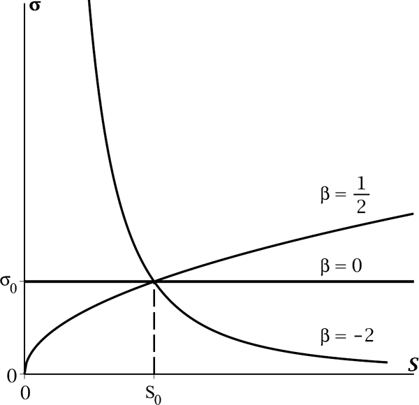
The local volatility function σ(S) = αSβ of the CEV model. The parameter α is chosen such that σ(S0) = σ0 is fixed.
The CEV process is a nonnegative process. To discuss its behaviour at the boundary points 0 and ∞, several definitions are required. For a diffusion process, {S(t)}t≥0, defined on an interval (a, b), we say that x = a and x = b are boundary points of the state space of the process. We say that point x ∈ {a, b} is
- (a) an entrance boundary if the process S can enter the state space starting from x but cannot reach x in finite time starting from the interior of the state space;
- (b) an exit boundary if the process S can reach x in finite time starting from the interior of the state space but cannot enter the state space starting from x;
- (c) a regular boundary if it is both an exit and an entrance boundary;
- (d) a natural boundary if it is neither an exit nor an entrance boundary.
We note that “entrance” really means entrance and not exit and “exit” means exit and not entrance. It is possible to impose a boundary condition for the diffusion S at a regular boundary. A regular boundary is called a killing (or reflecting) boundary when an instantaneously killing (or reflecting) boundary condition is imposed.
Given the CEV process satisfying (16.13), we can classify the boundary points 0 and ∞ according to the value of β. For β < 0, infinity is a natural boundary point. For , the origin is an exit boundary point. For , the origin is a regular boundary point. For β = 0, i.e., for GBM, both boundary points 0 and ∞ are natural boundaries. For β > 0, the origin is a natural boundary and infinity is an entrance boundary point.
16.1.2.2 Transition Probability Law
A combination of a change of variables and a scale and time transformation allows us to represent the CEV diffusion process {S(t)}t≥0 as a function of a squared Bessel (SQB) process {X(t)}t≥0, which has generator and hence satisfies the SDE
where μ is the so-called index of the process. The left-hand endpoint 0 is an entrance boundary if μ ≥ 0, a regular boundary if −1 < μ < 0, or an exit boundary if μ ≤ −1. The right-hand endpoint ∞ is a natural boundary. The state space of the SQB process is the interval [0, ∞) or (0, ∞) depending on the value of μ and the boundary condition at zero. The SQB diffusion is a time-homogeneous Markov process. The transition probability density function (PDF) is given by
where = μ if μ ≥ 0 or if μ ∈ (−1, 0) and 0 is specified as a regular reflecting boundary, and , μ < 0, if 0 is an exit or a regular killing boundary. Here, Iμ(z) denotes the modified Bessel function of the first kind, of order μ and argument z.
Let us find the transition PDF of the CEV process by reducing it to the SQB process as follows. First, a CEV process with a nonzero drift parameter ν is obtained from a driftless CEV process denoted {F (t)}t≥0 by means of a scale and time change:
Second, the change of variables via the monotonic mapping
gives us the SQB process X(t) := X(F (t)) = F (t)−2β /(α2 β2) with the index . Note that this mapping is strictly increasing for β < 0. Thus, the CEV diffusion can be expressed in terms of the SQB process as follows:
where the process {X(t)}t≥0 solves the SDE (16.14) with . Although the detailed mathematical proof of the representation (16.18) is left as an exercise for the reader, we briefly discuss the transformation. Two techniques are applied. First, the Itô formula is applied when transforming F (t) → X(t). Using the change of variables x = X(S) in the PDF (16.15) gives us the transition PDF of the driftless CEV process:
Second, the removal of drift is done with the use of the Kolmogorov PDE for the transition PDF. Denote the transition PDF of the CEV process with the drift parameter ν by p(ν)(t; S0, S). The function p(ν) solves the corresponding forward Kolmogorov PDE,
subject to the Dirac delta initial condition, p(ν)(0; S0, S) = δ(S − S0), and imposed homogeneous boundary conditions at the endpoints 0 and ∞. According to the transformation (16.16), the PDFs p(0) and p(ν) (with ν ≠ 0) relate to each other as follows:
The reader may check that p(ν) satisfies (16.20), assuming that p(0) solves Equation (16.20) with ν = 0. This proves that the process {S(t)}t≥0 in (16.16) satisfies the SDE (16.13) for the CEV process with drift. As a result, the PDF p(ν) is expressed in terms of the transition PDF pμ of the SQB process:
Assume that the parameter β is negative. Here, we consider the case when the endpoint S = 0 is a regular killing boundary (if β < −0.5) or exit (if −0.5 ≤ β < 0). The transition PDF p(0)(t; S0, S) with S0, S > 0 and t > 0 for the driftless CEV process F (t) takes the form
The density p(0)(t; S0, S) does not integrate (with respect to S) to 1, since S = 0 is an absorbing point. However, the driftless CEV diffusion process satisfies the martingale property:
For β < 0, the probability of absorption at zero (bankruptcy) is
where G(μ, a) is the complementary gamma function given by
Here, Γ(x) is the gamma function defined by .
Note that if the reflecting boundary condition is imposed at 0, then there is no absorption at the endpoint. The corresponding transition density (for the case with β < −0.5) is given by (16.23) with the replacement . The driftless process {F (t)}t≥0 becomes a strict submartingale.
16.1.2.3 Pricing European Options
We assume β < 0, so the driftless CEV process (with ν = 0) obeys the martingale property. Generally, we have
for all t, u ≥ 0. Therefore, the forward price process {e−νtS(t)}t≥0 is a martingale. Under the risk-neutral probability measure we set ν = r−q. The no-arbitrage price of a European call option (with expiry T and strike K) under the CEV process with the transition density in (16.19)–(16.23) is then given by
where
for the case when ν = r − q ≠ 0. If ν = 0, then and .
Proof
Using (16.23), we express the price of a European call under the CEV model as follows:
By changing variables defined by S′ = e−νT S, and then renaming the dummy variable S′as S,
Using (16.19) and applying the change of variables gives
where τ ≡ τT is given by (16.16), , , and . The formula (16.25) is deduced by applying (16.15) and changing variables in the above two integrals: , , and .
The two integrals in (16.25) can be computed numerically with the use of some quadrature rule. Alternatively, the call option pricing formula can be expressed in terms of the complementary noncentral chi-square distribution function. The latter can be represented as a series of elementary functions. When the call option price is calculated, the put option value can be obtained by using a put-call parity.
The noncentral chi-square distribution denoted is a continuous probability distribution with parameters υ ∈ (0, ∞) and λ ∈ [0, ∞) and with PDF
For integer υ, this distribution arises as a probability distribution of a sum of squared normal variables. Let Z1, Z2, ... , Zυ be independent standard normal random variables, and a1, a2, ... , aυ be some real constants, then is said to have the noncentral chi-square distribution with υ degrees of freedom and noncentrality parameter . If all aj = 0, then Y has the central chi-square distribution with υ degrees of freedom, which is denoted as usual by .
Since the integrands in (16.25) are both the noncentral chi-square PDFs of the form (16.26), the integrals in (16.25) can be expressed in terms of the complementary distribution function for :
Recall that the cumulative and complementary distribution functions, respectively denoted by F and Q, relate to each other as F (x) + Q(x) = 1.
The first integrand in (16.25) is the noncentral chi-square PDF with degrees of freedom and noncentrality parameter y0. Integrating with respect to y from m to infinity gives the corresponding complementary distribution function . The second integrand in (16.25) is equal to , where y is now the noncentrality parameter. The second integral is therefore equal to (see Exercise 16.4). Thus, the call option value is
The complementary noncentral chi-square distribution function Q(x; υ, λ) can be computed using the following formula:
where g(m, x) is a gamma PDF given by
16.1.3 The Heston Model
While in local volatility models a more realistic behaviour of asset prices is obtained by introducing a nonlinear volatility function, in the stochastic volatility framework, volatility changes over time according to another random process correlated with the asset price process. The volatility process is usually assigned through a suitable stochastic differential equation. Therefore, we deal with a two-dimensional SDE for asset price modelling. Let us denote the asset price by S(t) and the instantaneous variance (squared volatility) by v(t). In the Heston model, the asset price follows geometric Brownian motion and the variance is modelled as a square-root, mean-reverting diffusion with dynamics similar to the Cox–Ingersoll–Ross (CIR) model for interest rates. Thus, we consider the following two-dimensional model:
where the two Brownian motions are correlated, i.e., as dW1(t) dW2(t) = ρ dt. In reality, the correlation coefficient ρ is typically negative and can be close to −1. If ρ < 0, then volatility will increase when the asset price decreases. The parameters in (16.30)–(16.31) represent the following:
- μ is the rate of return on the asset.
- θ is the long variance, or long run average price variance; as t approaches infinity, the expected value of the variance v(t) goes to θ.
- κ is the rate at which v(t) reverts to θ.
- ξ is the volatility of the volatility; as the name suggests, this determines the variance of v(t).
To guarantee the positiveness of the instantaneous variance v(t), the model parameters satisfy
It is actually not easy to price derivatives under the Heston model. First, the joint distribution of the process (16.30)–(16.31) is not available in closed form. Therefore, the risk-neutral expectation of a payoff function is hard to compute. If the price process and volatility process are uncorrelated, then the price of a standard European option can be written as an integral over Black–Scholes prices. To develop derivative prices in the general case, one can use Monte Carlo simulations, PDE solutions, or transform methods. Stochastic-volatility models are quite popular among practitioners. Such models are able to produce pronounced volatility smiles. Since the model has two sources of uncertainty, namely, the movement of stock price S(t) and the movement of instantaneous variance v(t), the Heston model is incomplete. Further discussion of these techniques and the properties of the model is beyond the scope of this book.
16.2 Models with Jumps
16.2.1 The Poisson Process
Suppose that events of interest are occurring at random time moments. Let N(t) be the number of occurrences from time 0 to time t. By varying t ∈ ℝ+, we obtain a random process {N(t)}t≥0. Initially, we set N(0) = 0. Assume that only an individual event may occur at a time. Therefore, each possible realization (sample path) of N(t) is a nondecreasing step function that only changes by jumps of size 1. As a result, we obtain a fundamental pure jump process known as the Poisson process.
A Poisson process is an integer-valued stochastic process {N(t)}t≥0 with N(0) = 0 that satisfies the following properties.
- (a) The numbers of events that occur in disjoint time intervals are independent. That is, for all s1, s2, t1, t2 with 0 ≤ s1 < s2 ≤ t1 < t2 the random variables N(s2) − N(s1) and N(t2) − N(t1) are independent.
- (b) The distribution of the number of events that occur on a given time interval only depends on the length and does not depend on the location of the interval. That is, for all s and t with 0 ≤ s < t, the probability distribution of N(t) − N(s) depends on t − s and does not depend on t and s considered individually.
- (c) There exists a constant λ > 0 such that for any small interval of length δt, the probability of having one event occurring in a given small time interval, [t, t + δt], is approximately λ · δt plus an error of small order o(δt). That is,
whereas the probability to have two or more events occurring in [t, t + δt] is o(δt). That is,
Properties (a) and (b) mean that {N(t)}t≥0 is a process with independent and stationary increments. Additionally, as is shown just below, the above properties lead to the fact that all increments of the process {N(t)}t≥0 are Poisson distributed.
For all s and t such that 0 ≤ t < s,
Proof
The proof is left as an exercise for the reader.
Since N(0) = 0, Proposition 16.3 implies that the value N(t) for any t > 0 has the Poisson probability distribution Pois(λt). Therefore, the mean and variance of N(t) are equal,
respectively. In summary, the Poisson process is a process with independent, stationary, Poisson-distributed increments. The number λ is called the rate or intensity. For the Poisson process, the rate is equal to the average number of jumps per one unit of time, i.e.,
The Poisson process with rate λ is denoted by Nλ(t). Note that although we assume here that λ is constant, in general, the intensity can be a function of time t defined by
Let Ti be the occurrence time of the ith event or, equivalently, the moment when the Poisson process makes the ith jump. These random times T1, T2, ... form an increasing sequence of positive reals. Let us find the probability distribution of T1. The probability that T1 > t from some t > 0 is the same as the probability that no jumps occur in the interval [0, t]. So, we have
Therefore, the PDF of T1 is
for all t > 0, and zero otherwise, i.e., this is an exponential density where T1 ~ Exp(λ). Similarly, one can show that the increments Ti+1 − Ti are all Exp(λ) distributed. Additionally, one can show that all increments τi = Ti − Ti−1 with i = 1, 2, ... are independent.
This observation leads us to the second definition of the Poisson process presented just below. It is more constructive than the first one since it gives us a simple algorithm for generating sample paths.
Consider a sequence of i.i.d. exponentially distributed random variables, {τi}i≥1, having common mean . The Poisson process {N(t)}t≥0 is defined as
where for κ ≥ 1.
The process defined in (16.32) starts at zero; it makes a jump of size 1 at each time Ti, i.e., Ti is the moment of the ith jump. Each τi is a time lag between two successive jumps of the process. Note that the Poisson process {N(t)}t≥0 is a process with independent and stationary increments. Let us find the distribution of N(t) for t > 0. First, notice that for any κ ≥ 1 the occurrence time Tκ has the gamma distribution Gamma(κ, λ) with PDF
The probability of having at least κ jumps before time t is
Therefore, the probability of having κ jumps before time t is
Integration by parts gives
Therefore, for any κ = 0, 1, 2, ... That is, N(t) ~ Pois(λt). Similarly, using the memoryless property of the exponential distribution, one can show that N(t) − N(s) ~ Pois(λ(t − s)) for all t and s with 0 ≤ s < t. The result also follows from time stationarity where .
The Poisson process only changes its value at the time moments T1, T2, T3, ... forming a strictly increasing sequence 0 < T1 < T2 < T3 < .... The process is constant in between these jump times. According to the definition in (16.32), the sample paths are right-continuous, nondecreasing, piecewise-constant functions of time. A typical sample path is shown in Figure 16.2. The mean function of the Poisson process is a linear function of time: E[Nλ(t)] = λt. Finally, we define the compensated Poisson process {X(t) := Nλ(t)− λt}t≥0, which has zero mean function

16.2.2 Jump-Diffusion Models with a Compound Poisson Component
A standard Poisson process has deterministic jumps of size 1. A compound Poisson process is defined as a Poisson process with random jumps. Such a process is useful in insurance to model claims that arrive at time points generated by a Poisson process and the amounts claimed are positive random variables.
Let {N(t)}t≥0 be the Poisson process with intensity λ; let Y1, Y2, ... be a sequence of i.i.d. random variables with finite common mean E[Y]. Suppose that they are all independent of the Poisson process. The compound Poisson process, denoted {Q(t)}t≥0, is defined as
In the above example with claims made by policyholders to an insurance company, {Yκ}κ≥1 are the amounts claimed and N(t) is the number of claims made by time t. Then, Q(t) gives the total amount claimed by time t. The jumps in {Q(t)}t≥0 occur at the same time as the jumps in {N(t)}t≥0 but whereas the jumps in {N(t)}t≥0 are always of size 1, the jumps in {Q(t)}t≥0 are of random size. The κth jump that occurs at time Tκ is of size Yκ.
Properties of the compound Poisson process are similar to those of the standard Poisson process. The mean function of the compound Poisson process is linear in time as well:
Sample paths of the compound Poisson process are right-continuous, piecewise-constant functions of time. If the jumps Yκ are nonnegative (with probability one), then the sample paths are nondecreasing functions. Typical sample paths of a standard Poisson process and a compound Poisson process with jumps uniformly distributed in (0, 1) are given in Figures 16.3a and 16.3b, respectively.

The probability distribution of Q(t) can be derived by conditioning on the number of occurrences. Set for m ≥ 1. Then,
For example, it is not difficult to show that if all Yκ ~ Bin(1, p), 0 < p ≤ 1, then {Q(t)}t≥0 is a Poisson process with intensity λp.
Let us consider the following jump-diffusion model for asset prices. We assume that the log-price of the underlying asset follows Brownian motion with superimposed jumps:
where the standard Brownian motion {W (t)}t≥0 is independent of the compound Poisson component. Taking the exponential of both parts of (16.33) gives the asset price formula:
Since the exponential function takes strictly positive values, the price S(t) is strictly positive at every time t. As seen from (16.34), the asset price process follows geometric Brownian motion (with continuous paths) between the moments of jumps. At the moment of a jump, the asset price is multiplied by the exponential of the jump size, J ≡ eY . Thus, a sample path of S(t) is a piecewise continuous functions.
The asset price process (16.34) can be viewed as a solution to the stochastic differential equation with a Poisson component. The log-price, ln S(t), satisfies the SDE
As is seen, if no jump occurs, then the log-price simply evolves as a log-normal continuous process; if a jump occurs then the log-jump, Y ≡ ln J, is added to the log-price, i.e., the proportional change in the stock price is given by
When a jump occurs, the asset price S changes by S(J − 1), which is equivalent to multiplying S by J.
As we know, the asset price model is arbitrage free, if there exists an equivalent martingale measure (EMM). Under the EMM , the coefficient μ in (16.34) has to be selected such that holds for all t ≥ 0. Since W (t), N(t), and {Yi} are mutually independent, we have
where a := E[eY]. Therefore, under the EMM, the drift coefficient μ is given by
The jump size J ≡ eY can be taken to be a nonrandom number or a random variable. By assuming that J is log-normal (and hence the log-jump Y is normal), we obtain the Merton model. In the case of normal log-jumps, we can derive a closed-form pricing formula for standard (non-path-dependent) European options. Let all log-jumps Yi be independent normally distributed random variables with common mean α and variance β2. When the value of N(t) in (16.33) is fixed, the log-price ln S(t) becomes a sum of normal random variables and is therefore a normal variable as well. The distribution of the log-price ln S(t) conditional on the value of the Poisson process N(t) has mean
and variance
Thus, we have the conditional normal distribution
where Z ~ Norm(0, 1). Therefore, the value of S(t) conditional on N(t) = n can be rewritten as
Using the risk-neutral value of μ in (16.36) into (16.38) gives
where a ≡ E[eY] = eα+β2/2 since Y ~ Norm(α, β2). Hence, according to (16.37), the Merton asset price model (with fixed N(t) = n) can be reduced to the Black–Scholes model with an asset modelled as a GBM with an effective spot value and volatility .
The values of standard European options such as a call and put with strike K and expiry T are given by regular formulae. Let us denote the Black–Scholes (BS) option pricing function by . This is the pricing function for an underlying stock price following a GBM with spot value , volatility parameter , interest rate r, and stock dividend yield q. Now the option pricing function under the Merton jump-diffusion model, denoted υM , is obtained by taking the expectation of the BS option value with respect to N(T):
where and are given by (16.38) with t = T . Note that here we used the probability mass function of the Poisson random variable, .
16.2.3 The Variance Gamma Model
The variance gamma (VG) process is a three-parameter generalization of the Brownian motion model for the dynamics of the logarithm of the asset price. The VG process is obtained by evaluating the Brownian motion with drift at a random time given by a gamma process. The resulting process is a pure jump process.
Let {B(t; θ, σ) ≡ W(θ,σ)(t) = θt + σW (t)}t≥0 denote a scaled Brownian motion with drift rate θ and scale parameter σ, as defined in (10.23) of Section 10.3.1. Hence, this is a normal random variable,
The gamma process {G(t) ≡ G(t; μ, υ)}t≥0 with mean rate μ and variance rate υ is a random process starting at zero and with independent gamma distributed increments over nonoverlapping intervals of time. The increment ΔG = G(t + h) − G(t) over time interval [t, t + h] with 0 ≤ t < t + h has the gamma distribution with mean μh and variance υh. Its probability density is
Here, Γ(x) is the gamma function defined below Equation (16.24).
The VG process {X(t) ≡ X(t; σ, υ, θ)}t≥0 is obtained by evaluating the Brownian motion at a random time given by the gamma process with mean rate 1 and variance rate υ,
The process starts at zero: X(0) = 0. The PDF of the VG process at time t can be expressed by conditioning on the realization of the gamma time change G as a normal density function:
The unconditional probability density fX(t) of X(t) may then be obtained by employing the density (16.39), with h = t, for the time change g and integrating out g. This gives us the PDF in the following integral form:
The new specification for the stock price dynamics is obtained by replacing the role of Brownian motion in the original Black–Scholes geometric Brownian motion model by the variance gamma process. The stock price process is given by the geometric VG law with parameters σ, υ, and θ. The risk-neutral process for the asset price is given by
where r and q have the usual meaning, and the constant ω = ln(1 − θυ − σ2υ/2)/υ is chosen so that the discounted asset price process {e−(r−q)tS(t)}t≥0 is a martingale.
The price of a European-style derivative, υ(T, S) with spot S0 = S, time to maturity T , and payoff Λ, is given by the usual risk-neutral pricing formula, , where the expectation is taken under the risk-neutral measure. The evaluation of the derivative price proceeds by conditioning on the random time change G(T), which is independent of the Brownian motion. Conditional on the value of G(T), the VG process X(T) is normally distributed. Thus, the asset price S(t) conditional on time G(t) = g is log-normal:
where . Thus, the option value with the asset price S at the expiry time g is given by the Black–Scholes formula. Let υBS denote the Black–Scholes derivative pricing function. The derivative price with expiry T under the VG risk-neutral dynamics, denoted υVG, is then obtained by integrating this conditional Black–Scholes price with respect to the gamma time change:
The latter integral can be evaluated numerically.
16.3 Exercises
Exercise 16.1. Let the process {F (t)}t≥0 solve the SDE
Show that the process {X(t)}t≥0 defined by X(t) := (F(t))−2β/(α2 β2) is an SQB process with index , i.e., it satisfies the SDE (16.14).
Exercise 16.2. Suppose that p(0)(t; S0, S) solves the PDE
with σ(S) = αSβ+1. Show that the function p(ν) defined by
with and ν ≠ 0 satisfies the PDE
Exercise 16.3. Let {F(t)}t≥0 be a forward price process solving the SDE
with some nonlinear σ(F). Consider a transformed process S(t) = ertF(τt) with some strictly increasing smooth function τt such that
The function τ is a time change. The transition PDF p(r) for the process {S(t)}t≥ is given by
where p(0) is a transition PDF of the forward price F . Show the following.
(a) The PDF p(r) satisfies the forward Kolmogorov PDE
where is a time- and state-dependent function. The process {S(t)}t≥0 hence solves the time-inhomogeneous SDE
(b) Show that holds (hence is time homogeneous) only if τt solves the ordinary differential equation (ODE)
subject to the initial conditions (16.42).
(c) The solution to (16.43) is independent of S only if the function σ(F) satisfies
The only solution to this ODE is a power function: σ(F) = αFβ+1, where α and β are constants. The respective solution to (16.43) is .
Thus, the CEV process is the only model where the above scale and time change give a time-homogeneous diffusion with linear drift. Moreover, the transformation in this case is volatility preserving, i.e., .
Exercise 16.4. Prove the following property of the noncentral chi-square PDF:
Hint: Use the following identities:
where .
- Exercise 16.5. Prove that the compensated Poisson process, {Nλ(t) − λt}t≥0, is a martingale with respect to its natural filtration.
- Exercise 16.6. Consider the exponential process {exp(at + Nλ(t))}t≥0. For what value of a is this process a martingale with respect to its natural filtration?
Exercise 16.7. Apply the following integral representation of the modified Bessel function of the second kind (of order ν), denoted Kν, to find a closed-form nonintegral expression for the transition PDF of the VG process:
- Exercise 16.8. Consider the Heston model (16.30)–(16.31) with uncorrelated Brownian motions W1 and W2.
- (a) Show that the instantaneous variance v(t) in (16.31) can be expressed in terms of the SQB process by means of a suitable scale and time change.
- (b) Find the transition PDF of the variance process v(t).
- (c) Write the price of a standard European option with payoff Λ as an integral over the Black–Scholes prices.
1 In physics, elasticity is the ability of a deformed material body to return to its original shape and size when the forces causing the deformation are removed.