
Portfolio Management
3.1 Expected Utility Functions
3.1.1 Utility Functions
Suppose we have different investment opportunities to choose from. These investments may affect our future wealth. For example, the task is to allocate an initial capital among several risky assets to form an investment portfolio. Once we decide on such a risky investment, the future wealth becomes uncertain so it follows some probability distribution. The investment selection procedure can be reduced to the optimization of the probability distribution of the uncertain future wealth. If the outcomes from all alternatives were certain, then we would select the investment that produces the largest return. For the case with uncertain outcomes, we may be interested in minimizing the variance of the respective probability distribution but other criteria can be applied. So we need a systematic way to rank random wealth levels. In the case of alternatives with uncertain outcomes, we introduce some score function that is calculated as an expected value of a so-called utility function.
Suppose we are given a function u: ℝ → ℝ so that each possible investment can be assessed by computing the expected utility value E[u(V)] of the future wealth V . In other words, the value of an investment can be measured by the expected value of the utility of its consequences. To compare possible alternatives, we first compute E[u(V)] for each possible wealth function V and then choose an alternative with the greatest expected utility value. The specific utility function used depends on individual investment preferences, risk tolerance, and individual financial environment. The simplest example of a utility is the linear function u(x)= x. Whoever uses this utility function ranks uncertain wealths by their expected values.
Here are some of the most commonly used utility functions (see Figure 3.1):
- the logarithmic (log) utility function u(x) = ln x;
- the exponential utility function u(x) = −e−ax with a > 0;
- the power utility function u(x)= xa with 0 < a < 1;
- the quadratic utility function u(x)= x − ax2 with 0 < a defined for x<12a.

As you can see, some utility functions can take negative values. This negativity does not matter since an investor ranks investments using relative values. Moreover, the addition of a constant to a utility function and the multiplication of a utility function by a positive constant do not affect the rankings. If for some utility function u and two investments V1 and V2 we have that E[u(V1)] ≤ E[u(V2)], then for any a ∊ ℝ and b > 0 we obtain
E[a+bu(V1)]=a+bE[u(V1)]≤a+bE[V2]=E[a+bu(V2)].
In general, given a utility function u, we can define another utility function ˜u of the form
˜u(x)=a+bu(x)
with b > 0. This new utility function ˜u is said to be equivalent to u. Equivalent utility functions give identical rankings of investment opportunities.
Another example of a utility function is the linear utility u(x)= a + bx, b > 0. This function reflects expectations of a risk-indifferent investor. For any random wealth V we have
E[u(V)]=E[a+bV]=a+bE[V]=u(E[V]),
hence the linear utility function has no preference for a deterministic wealth or for a random wealth provided that expected wealths are the same.
Example 3.1.
An investor with total capital W can invest any amount between 0 and W . If an amount is invested, then the same amount is either won or lost with respective probabilities p and 1 − p. In other words, with probability p, the investor doubles the initial investment; with probability 1 − p, the investor loses all the invested money. What amount should be invested if the log utility function u(V) = ln V is utilized for ranking alternatives?
Solution. Let the amount of xW for some 0 ≤ x ≤ 1 be invested. The investor's final fortune V (x) is either W + xW or W − xW with respective probabilities p and 1 − p. Hence the expected utility of the final wealth is
E[u(V(x))]=ln(W+xW)p+ln(W−xW)(1−p)=ln((1+x)W)p+ln((1−x)W)(1−p)=ln(1+x)p+ln(1−x)(1−p)+lnW.
To find the optimal value of x, let us differentiate E[u(V (x))] with respect to x and then find zeros of the derivative obtained:
ddxE[u(V(x))]=ddx(pln(1+x)+(1−p)ln(1−x))=d1+x−1−p1−x=2p−(1+x)1−x2.
If p∈(0,12], then the derivative is strictly negative for all x ∊ (0, 1) and the expected utility attains its maximum value at x = 0. In this case, the risk to lose the invested amount is too high, and it is reasonable to invest nothing. If p∈(12,1), then the derivative is zero at x* = 2p − 1 ∊ (0, 1). The second derivative of the expected utility function is negative at x* , hence x = 2p − 1 ∊ (0, 1) is the point of maximum of V (x). Therefore, 100(2p − 1)% of the initial capital is to be invested. For example, for p = 70%, the investor shall invest 40% of the fortune.
Example 3.2.
The Saint Petersburg Paradox, originally proposed by Nicolaus Bernoulli, is a classical example of how utility functions are used in the decision making process. Consider a game of chance where a fixed fee is paid to enter, and then a fair coin will be tossed repeatedly until a head first appear ending the game. The payoff starts at $1 and then is doubled every time a tail appears. As a result, the player wins $2k−1 if a head first appears on the kth toss (k = 1, 2, 3,...). How much should the player be willing to pay to enter such a game?
Solution. First, let us find the expected value of the payoff. We deal with a sequence of independent trials where the probability of success (i.e., a head occurs) is 12. With probability p1=12, a head first appears on the first toss and the player wins $1; with = probability p2=14, a head first appears on the second toss and the player wins $2; with = probability p3=18, a head first appears on the third toss and the player wins $4, etc. The probability that a head first appears on the kth toss is pk = 2−k; the payoff is then $2k−1. Therefore, the expected payoff is then
E=12⋅1+14⋅2+18⋅4+⋯+12k2k−1+⋯=12+12+12+⋯=∞.
The expected win for the player of this game is an infinite amount of money. So no matter how large is the fee paid to enter this game, the player will eventually make a profit in the long run repeatedly playing this game. The classical solution to this “paradox” is to assume that one's valuation of money is different from its face value and depends on his or her wealth. Let us apply the logarithmic utility model to find a reasonable price c charged to enter the game. Let the initial wealth of the player be denoted V0. The expected log utility function of the total wealth V = V (c) after playing the game is
E[lnV]=∞∑k=1ln(V0+2k−1−c)12k<∞.

An outcome tree for the St. Petersburg game. The game consists of a series of coin tosses offering a 50% chance of winning $1, a 25% chance of $2, a 12.5% chance of $4, and so on. The gamble may continue indefinitely.
A rational player is willing to play the game only if the game will not decrease the expected utility of the wealth:
E[lnV]≥E[lnV0].
After plotting the expected change in utility,
E[lnV]−E[lnV0]=E[lnV−lnV0]=E[ln(V/V0)],
as a function of the cost c, we observe that E[ln(V (c)/V0)] is a strictly decreasing function of c and there exists a maximum cost c* so that any price c<c gives a positive expected change in utility. Such a cost c* depends on the initial capital V0 and can be found by solving E[ln(V (c)/V0)]=0 for c. For example, a person with $2 in his pocket is willing to pay up to $2, a person with $1000 is willing to pay up to $5.97, and a millionaire is willing to pay up to $10.94.
3.1.1.1 Risk Aversion
Utility functions are constructed based on the following principles.
Principle 1. Investors prefer more to less. If there are two certain wealths V1 and V2, then an investor prefers the larger one, i.e., V1 <V2 implies u(V1) <u(V2). Hence, u is an increasing function.
Principle 2. Investors are averse to risk. Positive deviations ΔV from average wealth V cannot compensate for equally large and equally probable negative deviations −ΔV from average wealth, i.e., u(V) − u(V − ΔV) > u(V +ΔV) − u(V). Therefore,
u(V)>u(V+ΔV)+u(V−ΔV)2. (3.1)
The inequality in (3.1) holds true for all V if u is a concave function. The left-hand side, u(x) − u(V − ΔV), is “the pain of losing ΔV dollars,” and the right-hand side, u(V + ΔV) − u(V), is “the joy of winning ΔV dollars.” The inequality says that the pain of losing outweighs the joy of winning, alternatively that we react more severely to a loss then we do to a gain of the same magnitude.
Suppose that there are two alternatives for future wealth: the first provides either x or y each with a probability of 12, the second gives 12x+12y with certainty. Although both alternatives have the same expected value, a risk-averse investor prefers the certain wealth of 12x+12y to a 50-50 chance of x and y: u(12x+12y)≥12u(x)+12u(y).
Recall that a function u defined on an interval [a, b] is said to be concave if for any α with 0 ≤ α ≤ 1 and any x, y ∊ ℝ there holds
u(αx+(1−α)y)≥αu(x)+(1−α)u(y).
A function u is said to be convex on [a, b] if the function −u is concave on [a, b]. That is, if for any α with 0 ≤ α ≤ 1 and any x, y ∊ ℝ there holds
u(αx+(1−α)y)≤αu(x)+(1−α)u(y).
A twice differentiable function u is concave (convex) on an interval [a, b] if its second derivative u″ is nonpositive (nonnegative) on [a, b]. A utility function is said to be risk-averse (on an interval [a, b]) if it is concave (on the interval [a, b]). A concave function is depicted in Figure 3.3. For a twice-differentiable utility function, the risk-averse condition means that the second derivative of the utility function is nonpositive.

The concave (or convex-upward) plot of a typical risk-averse utility function. As is seen, every curve segment of a concave plot lies above a chord connecting the endpoints of the segment.
Recall Jensen's inequality: let u be a concave function, then for any random variable V,
E[u(V)]≤u(E[V]). (3.2)
This means that a risk-averse investor prefers a certain wealth of W to an uncertain wealth V with the same expected value E[V]= W . This observation relates to the notion of the certainty equivalent.
The certainty equivalent of an uncertain wealth V is defined as the amount of a constant wealth C that has the utility level equal to the expected utility of V :
u(C)=E[u(V)]. (3.3)
Clearly, the certainty equivalent is the same for all equivalent functions. Combining (3.2) and (3.3) gives that the certainty equivalent is always less than the expected value of the wealth for a risk-averse investor with a concave utility function:
u(C)≤u(E[V])⇒C≤E[V].
Let us represent the uncertain return V in the form V = W + ∈ where W is the initial capital and ∈ is a zero-mean risk. A natural way to measure risk aversion is to ask how much an investor is ready to pay to get rid of the zero-mean risk ∈. This price, called a risk premium and denoted π, is defined implicitly by
E[u(W+∈)]=u(W−π). (3.4)
Let us consider a small risk ∈. Expanding the left-and right-hand sides of (3.4) in Taylor's approximations gives
E[u(W+∈)]≈E[u(W)+∈u′(W)+∈22u″(W)]=u(W)+E[∈]u′(W)+E[∈2]2u″(W)=u(W)+σ2∈2u″(W)
and
u(W−π)≈u(W)−πu′(W),
respectively, where σ2∈:=E[∈2] is the variance of ∈. Substituting these back into (3.4), we obtain
π≈σ2∈2Au(W),
where
Au(W):=−u″(W)u′(W)
is the Arrow–Pratt absolute risk aversion coefficient. We say that investor 1 (with utility function u1) is more risk averse than investor 2 (with utility function u2) if for the same initial wealth W and zero-mean risk ∈, the risk premium π1 paid by investor 1 is larger than the risk premium π2 of investor 2, or, equivalently, Au1(W)>Au2(W).
The degree of risk aversion can be viewed as a measure of the magnitude of concavity of the utility function: the stronger the bend in the function, the larger the risk aversion coefficient A. For example, the risk-aversion coefficient for a linear utility function, u(V)= a + bV, is zero. The coefficient A is normalized by the derivative u′ that appears in the denominator. This makes A independent of linear transformations of the utility function u. Indeed, for any reals a and b ≠ 0 we have
−(a+bu(x))''(a+bu(x))'=−bu″(x)bu′(x)=−u″(x)u′(x).
The coefficient function A(W) shows how risk aversion changes with the wealth level. It is usually argued that absolute risk aversion should be a decreasing function of wealth. That is, many investors are willing to take more risk when they are financially secure. For example, a lottery to gain or lose $100 is potentially life-threatening for an investor with initial wealth W = 101, whereas it is negligible for an investor with wealth W = 100,000. The former individual should be willing to pay more than the latter for the elimination of such a risk. Thus, we may require that the risk premium associated with any risk is decreasing in wealth. It can be shown that this holds if and only if the Arrow–Pratt absolute risk aversion coefficient is decreasing in wealth. This requirement means that
A′(W)=−u‴(W)u′(W)−u″(W)2u′(W)2<0.
A necessary condition for this to hold is u′″ (W) > 0.
As a specific example, consider the exponential utility function u(x)= −e−ax. Differentiate it to obtain
u′(x)=ae−axandu″(x)=−a2e−ax.
Therefore, we have A(x)= −u″ (x)/u′ (x)= a. In this case, the risk aversion remains constant as wealth increases. As another example, consider the power utility function u(x)= xa with 0 < a < 1. We have u′ (x)= axa−1 and u″ (x)= a(a−1)xa−2. Thus, A(x)= (1−a)/x. So risk aversion decreases as wealth increases. Similarly, for the logarithmic utility function u(x) = ln x, we have u′ (x)=1/x, u″ (x)= −1/x2, and A(x)=1/x.
3.1.2 Mean-Variance Criterion
Suppose that the optimal investment opportunity is chosen by maximizing the expected utility of the wealth. Let us show how the utility maximization method reduces to the mean-variance criterion when an optimal investment is selected by maximizing the expected wealth and minimizing the variance of the wealth. Suppose that the final wealth follows a normal probability distribution and the investor uses an exponential utility function u(x)= −e−ax with a > 0. Recall that the mathematical expectation of an exponential function of a normal random variable Z can be expressed in terms of the expected value and variance of Z as follows:
E[eZ]=eE[Z]+Var(Z)/2.
If the wealth V is normal, then −aV is normal as well with mean E[−aV]= −aE[V] and variance Var(−aV)= a2 Var(V). Therefore, the expected utility of the wealth V is
E[u(V)]=−exp(−aE[V]+a2Var(V)/2)=−exp(−a(E[V]−aVar(V)/2)).
The exponential function is increasing. Thus, the expected utility is maximized by choosing an investment that maximizes E[V] − a Var(V)/2. This means that alternative investments can be ranked by comparing their means and variances. If there are two investments so that E[V1] ≥ E[V2] and Var(V1) ≤ Var(V2), then the first investment results in a larger expected utility than does the second: E[u(V1)] ≥ E[u(V2)].
One can arrive at the same conclusion for the case of a quadratic utility function u(x)= x − ax2 with a > 0. Assuming that the wealth V satisfies V<12a, the expected utility E[u(V)] is maximized by selecting an investment with a larger expected wealth and smaller variance Var(V).
To deal with a general utility function u, let us consider the Taylor expansion of u about the point E[V]:
u(V)≈u(E[V])+u′(E[V])(V−E[V])+12u″(E[V])(V−E[V])2.
Taking expectations gives
E[u(V)]≈u(E[V])+u′(E[V])E[V−E[V]]+12u″(E[V])E[(V−E[V])2]=u(E[V])+u″(E[V])Var[V]/2. (3.5)
Here we use that E[V − E[V]] = E[V] − E[V] = 0 and E (V − E[V])2 = Var(V). Therefore, a reasonable approximation to the optimal investment is given by an investment that maximizes
u(E[V])+u″(E[V])Var[V]/2.
Suppose that u″ (x) is a nondecreasing function in x. Then, since u″ (x) ≤ 0, an optimal investment V can be again selected by both maximizing the expected value E[V] and minimizing the variance Var(V). Recall that the standard deviation σV=√Var(V) characterizes the risk associated with the investment V. Therefore, the mean-variance criterion tells us that the optimal investment is attained by maximizing the expected value of the wealth and minimizing the risk.
3.2 Portfolio Optimization for Two Assets
3.2.1 Portfolio of Two Assets
In a one-period setting, let us consider a model with two risky assets A1t and A2t, where t ∊{0,T}. Each asset, labelled by i = 1, 2, is characterized by its initial value Ai0 and the respective single-period return ri=AiT−Ai0Ai0. At that we have AiT=Ai0(1+ri). The risky returns r1 and r2 (as well as the terminal asset prices A1T and A2T) are random variables defined on a common probability space with state space and probability function ℙ.
Let us form a portfolio [x1,x2]Τ by purchasing x1 shares of asset 1 and x2 shares of asset 2. The initial wealth of such a portfolio is V0=x1A10+x2A20. The (one-period) rate of return rV is then given by
rV=VT−V0V0=x1(A1T−A10)+x2(A2T−A20)V0=x1(A1T−A10)A10A10V0+x2(A2T−A20)A20A20V0=x1A10V0r1+x2A20V0r2.
Introduce the following weights:
w1=x1A10V0andw2=x2A20V0
which are called the allocation weights of funds between the two underlying assets. In other words, 100wi% of the initial wealth is invested in asset i = 1, 2. By the definition of a wealth function, the weights add up to one: w1 + w2 = 1. If short selling is allowed, then one of the weights may be negative and, hence, the other weight is greater than one. For a portfolio without short selling, both weights are between zero and one. Being given the values of returns ri and weights wi, the total wealth at the end of the period is
VT=(1+rV)V0=(1+w1r1+w2r2)V0=(w1(1+r1)+w2(1+r2))V0.
A portfolio with weights [w1,w2]Τ can be characterized by the expected return and the variance of the return. Since rV = w1r1 + w2r2, we have that
E[rV]=E[w1r1]+E[w2r2]=w1E[r1]+w2E[r2] (3.6)
Var(rV)=Var(w1r1)+Var(w2r2)+2Cov(w1r1,w2r2)=w21Var(r1)+w22Var(r2)+2w1w2Cov(r1,r2)=w21Var(r1)+w22Var(r2)+2w1w2Corr(r1,r2)√Var(r1)√Var(r2). (3.7)
Here, we define the coefficient of correlation between two random variables as follows:
Corr(r1,r2)=Cov(r1,r2)√Var(r1)Var(r2)∈[−1,1].
Note that if the variance of one of the random variables is zero then the correlation coefficient is undefined.
The variance of the return on a portfolio without short selling (i.e., both w1 and w2 are nonnegative) cannot exceed the greater of the variances of the underlying asset returns:
0≤Var(rV)≤max{Var(r1),Var(r2)}.
Proof. Since the value of the correlation coefficient is always between −1 and 1, from (3.7) we obtain that
Var(rV)≤w21Var(r1)+w22Var(r2)+2w1w2√Var(r1)√Var(r2)≤(w1√Var(r1)+w2√Var(r2))2≤(w1+w2)2max{Var(r1),Var(r2)}=max{Var(r1),Var(r2)}.
On the other hand, the variance is always a nonnegative quantity.
Introduce the following notation for the expected returns, the variances of returns, and the correlation coefficient:
μi=E[ri],σ2i=Var(ri);(i=1,2);ρ12=Corr(r1,r2).
Moreover, denote μV=E[rV]andσ2V=Var(rV). In this notation, Equations (3.6) and (3.7) take the respective forms:
μV=w1μ1+w2μ2andσ2V=w21σ21+w22σ22+2ρ12w1w2σ1σ2. (3.8)
Consider two risky assets with the following probability distributions of their returns:
Scenario ω |
Probability ℙ(ω) |
Return r1 |
Return r2 |
|---|---|---|---|
ω1 |
0.1 |
−20% |
30% |
ω2 |
0.6 |
5% |
10% |
ω3 |
0.3 |
10% |
−20% |
Calculate the expected returns, μi, standard deviations, σi, and correlation coefficient of returns, ρ12.
Solution. To compute the mathematical expectation of a random variable X on a finite sample space Ω, we use the formula
E[X]=∑ω∈ΩX(ω)ℙ(ω).
The expected returns are
μ1=E[r1]=3∑i=1r1(ωi)ℙ(ωi)=(−0.2)⋅0.1+0.05⋅0.6+0.1⋅0.3=0.04=4%,μ2=E[r2]=3∑i=1r2(ωi)ℙ(ωi)=0.3⋅0.1+0.1⋅0.6+(−0.2)⋅0.3=0.03=3%.
Using the fact that Var(X) = E[(X − E[X])2] and Cov(X, Y) = E[(X − E[X])(Y − E[Y])], we similarly obtain:
Var(r1)=(−0.2−0.04)2⋅0.1+(0.05−0.04)2⋅0.6+(0.1−0.04)2⋅0.3=0.0069,Var(r2)=(0.3−0.03)2⋅0.1+(0.1−0.03)2⋅0.6+(−0.2−0.03)2⋅0.3=0.02610,Cov(r1,r2)=(−0.2−0.04)⋅(0.3−0.03)⋅0.1+(0.05−0.04)⋅(0.1−0.03)⋅0.6+(0.1−0.04)⋅(−0.2−0.03)⋅0.3=−0.0102.
The standard deviations are
σ1=√Var(r1)=√0.0069≅0.08307,σ2=√Var(r2)=√0.02610≅0.16156.
The correlation coefficient ρ12 is
ρ12=Cov(r1,r2)√Var(r1)Var(r2)≅−0.01020.08307⋅0.16156≅−0.76007≅−76%.
Example 3.4.
Find an optimal allocation of the initial wealth V0 = 1000 between two risky assets from Example 3.3 when attempting to maximize the expected value, E[u(VT)], of an exponential utility function u(x) = 1 − e−0.01x of the wealth VT.
Solution. Let the weights of a portfolio V in the two assets be w1 = x and w2 = 1 − x, respectively. The return on such a portfolio is rV (x)= xr1 + (1 − x)r2. At the end of the period, the portfolio value is VT = V0(1 + rV). Now we can find the optimal allocation by solving the following maximization problem:
E[u(VT)]=E[1−e−0.01VT]=E[1−e−0.01V0(1+rV)]=1−E[e−10(1+xr1+(1−x)r2)]→maxx.
It is equivalent to minimizing E[e−10(1+xr1+(1−x)r2)] w.r.t. x. Evaluate the mathematical expectation:
E[e−10(1+xr1+(1−x)r2)]=3∑i=1pie−10(1+xr1(ωi)+(1−x)r2(ωi))=0.1e−13+5x+0.6e−11+0.5x+0.3e−8−3x.
Differentiate the expected value w.r.t. x and equate the obtained derivative to zero:
0.5e−13+5x+0.3e−11+0.5x−0.9e−8−3x=0.
The resulting equation can be solved numerically to yield the optimal value x*≅0.67431, where the expected utility function attains its maximum value. Therefore, the optimal allocation weights are w1 ≅ 67.431% and w2 ≅ 32.569%.
3.2.2 Portfolio Lines
Consider two risky assets with respective returns r1 and r2. It is a typical situation when the joint probability distribution of the returns is unknown. However, it may be possible to estimate the moments of the returns from historical data. Suppose we only know the expected returns and variances of the returns, μi,σ2i,i=1,2, and the correlation coefficient ρ12. Every portfolio in these assets can be characterized by its expected return and variance of its return.
On the (σ, μ)-plane, a portfolio V with allocation weights [w1,w2]Τ is represented by a point whose coordinates (σV, μV) are calculated by (3.8). Let us find a set of points on the (σ, μ)-plane that describes all possible portfolios in the two underlying assets. Since w1 + w2 = 1, all portfolios can be parameterized by a single variable x ∊ ℝ: w1 = x and w2 = 1 − x. Therefore, the set of all possible portfolios can be represented by a portfolio line (which can shrink to a single point in some extreme cases). Equations (3.8) can be rewritten as follows:
μV(x)=xμ1+(1−x)μ2,σ2V(x)=x2σ21+(1−x)2σ22+2x(1−x)σ1σ2ρ12 (3.9)
with x ∊ (−∞, ∞). For portfolios without short selling (i.e., w1 ≥ 0 and w2 ≥ 0), we have that 0 ≤ x ≤ 1.
3.2.2.1 Case with |ρ12| = 1
First, let ρ12 = 1. Then from (3.9) we obtain that the variance of return on portfolio V is given by σ2V(x)=(xσ1+(1−x)σ2)2, and hence σV (x)= |xσ1 + (1 − x)σ2|. The portfolio line is described by
σV(x)=|x(σ1−σ2)+σ2|andμV(x)=xμ1+(1−x)μ2,x∈ℝ.
Let us assume that μ1 ≠ μ2 and σ1 ≠ σ2 (we leave the other cases as exercises for the reader). We can solve the second equation for x to obtain x=μV−μ2μ1−μ2. Substituting this expression in the formula for σV gives us the following relationship:
σV=|σ2+(σ1−σ2)μV−μ2μ1−μ2|⇒σV=|σ1−σ2σ1−μ2μV+σ2μ1−σ1μ2μ1−μ2|.
As we can see, the standard deviation σV is a piecewise-linear function of μV :
σV={aμV+bifμV≥−ba,−(aμV+b)ifμV<−ba,wherea:=σ1−σ2μ1−μ2andb:=σ2μ1−σ1μ2μ1−μ2.
The plot of σV as a function of μV is a broken line with two half-lines. It is interesting to observe that there is a portfolio with zero variance (i.e., a risk-free portfolio). Indeed, σV=0iffμV=σ2μ1−σ1μ2σ1−σ2. The weights w1 = x and w2 = 1 − x can be obtained by solving the equation xσ1 + (1 − x)σ2 = 0 for x. Hence, the weights of a risk-free portfolio are
ˆw1=σ2σ2−σ1andˆw2=σ1σ1−σ2. (3.10)
One of the weights is negative, hence short selling is necessary to construct a risk-free portfolio.
Now let us find what part of the portfolio line corresponds to portfolios without short selling. The portfolios with weights (0, 1) and (1, 0) are the endpoints of such a set. By changing x from 0 to 1, we continuously move the point along the line of portfolios without short selling from one endpoint to the other. Since the portfolio with σV = 0 has a negative weight, the no-short-selling line is a segment lying on one of two rays. The final result of our analysis is presented in Figure 3.4a.
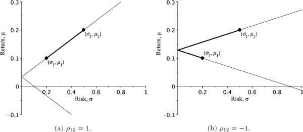
A typical portfolio line for the case with |ρ12| = 1. The bold part indicates portfolios without short selling.
Similarly, we can construct the portfolio line for the case with ρ12 = −1. The portfolio line is described by
σV(x)=|x(σ1+σ2)−σ2|andμV(x)=xμ1+(1−x)μ2withx∈ℝ.
By excluding x from the above equations, we obtain
σV=|σ1+σ2μ1−μ2μV−σ2μ1+σ1μ2μ1−μ2|.
Again, the plot of σV as a function of μV is a broken line. Now σV = 0 iff μV=σ2μ1+σ1μ2σ1+σ2.
The weights of the risk-free portfolio are
ˆw1=σ2σ1+σ2andˆw2=σ1σ1+σ2. (3.11)
Both weights are positive, so no short selling is required to construct a portfolio with a zero variance of return. The no-short-selling line is a broken line segment lying on both half-lines. The result of our analysis is given in Figure 3.4b.
3.2.2.2 Case with |ρ12| < 1
Excluding x from (3.9) and expressing σ2 as a function of μ gives
σ2=(μ−μ2)2(μ1−μ2)2σ21+(μ−μ1)2(μ1−μ2)2σ22−2(μ−μ1)(μ−μ2)(μ1−μ2)2σ12σ1σ2.
After doing some algebra, we can bring this equation to the form:
σ2=Aμ2−2Bμ+C,whereA=σ21−2ρ12σ1σ2+σ22(μ1−μ2)2,B=μ1σ22+μ2σ21−2ρ12σ1σ2(μ1+μ2)(μ1−μ2)2,C=(μ1σ2)2+(μ2σ1)2−2ρ12σ1σ2μ1μ2(μ1−μ2)2.
The curve defined by the above equation is a hyperbola. Indeed, let us rewrite the equation as follows: σ2=A(μ−BA)2+D, where D=C−B2A. By changing variables from (σ, μ) to (x=σ√D,y=√A√Dμ−B√AD), one can easily obtain the canonical equation of a hyperbola: x2 − y2 = 1. A typical portfolio line is given in Figure 3.5.
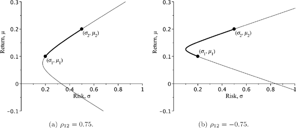
A typical portfolio line for the case with −1 < ρ12 < 1. The bold part indicates portfolios without short selling.
As is seen from Figures 3.4 and 3.5, the plot of a portfolio line is a hyperbola for the case with ρ12 ∊ (−1, 1) and a broken line for the extreme case with |ρ12| = 1. The evolution of a portfolio line when μ1,2 and σ1,2 are fixed and ρ12 is changing from −1 to 1 is represented in Figure 3.6.
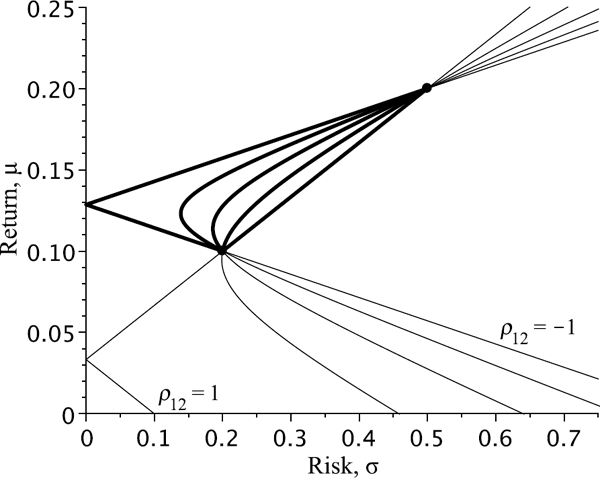
Portfolio lines for varying ρ12 and fixed μ's and σ's. The parameter ρ12 is changing from −1 to 1 with the step size of 0:5. The bold parts indicate portfolios without short selling.
3.2.2.3 Case with a Risk-Free Asset
Suppose that one of two assets (say, asset 2) in our portfolio is risk-free, that is, the variance of its return is zero: σ22=Var(r2)=0. Hence, the return r2 is constant: r2 ≡ r.
The formula of the variance in (3.9) reduces to σ2V(x)=x2σ21 or just σV(x)=|x|σ1. So the standard deviation σV of such a portfolio depends on the weight w1 of the risky asset as follows: σV = |w1|σ1. The portfolio line is described by a piecewise linear function: σV=σ1|μV−rμ1−r|. Thus, the portfolio plot is a broken line with its vertex at the point that corresponds to the risk-free asset (see Figure 3.7).
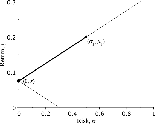
Portfolio line for one risky and one risk-free asset. The risk-free rate of return is r. The bold part indicates portfolios without short selling.
3.2.3 The Minimum Variance Portfolio
As is seen in Figures 3.4 and 3.6, there is always a portfolio with the smallest possible variance σ2V. We already found risk-free portfolios with zero variance for the case with |ρ12| = 1. Let us now find the general solution to this problem.
Suppose that |ρ12| < 1 or σ1 ≠ σ2 holds. The portfolio with the minimum variance is attained at
ˆw1=σ22−ρ12σ1σ2σ21+σ22−ρ12σ1σ2andˆw2=σ21−ρ12σ1σ2σ21+σ22−ρ12σ1σ2. (3.12)
The variance of the portfolio is
σ2mv=(1−ρ212)σ21σ22σ21+σ22−2ρ12σ1σ2. (3.13)
Proof. By differentiating the variance σ2V given by (3.9) w.r.t. x and equating the derivative to zero, we obtain the following linear equation for x:
dσ2Vdx=2(σ21+σ22+2ρ12σ1σ2)x−2(σ22−ρ12σ1σ2)=0.
The solution is
x0=σ22−ρ12σ1σ2σ21+σ22−2ρ12σ1σ2. (3.14)
Thus, for the weights ˆw1=x0 and ˆw2=1−x0, we immediately obtain (3.12). Since the second derivative of σV2 w.r.t. x is positive everywhere:
d2σ2Vdx2=2(σ21+σ22−2ρ12σ1σ2)>0,
the variance σV2 attains its smallest value at x0. Substituting x0 in (3.8) gives us Equation (3.13) for the minimum variance.
Clearly, the formulae in (3.12) and (3.13) work for both cases when |ρ12| = 1 or |ρ12| < 1. If |ρ12| = 1, then σmv2 = 0 in (3.13) and the formulae in (3.12) reduce to (3.10) or (3.11) depending on the sign of ρ12.
3.2.3.1 Case without Short Selling
While proving Theorem 3.2, we did not take into account whether short sells are allowed. Let us find the minimum variance portfolio without short sells, i.e., with nonnegative weights. The function σV2 in (3.9) attains its minimum value on [0, 1] either at one of the boundary points x ∊{0, 1} or at the point x0 given by (3.14) provided 0 <x0 < 1. Both weights ˆw1 and ˆw2 in (3.12) are positive iff ρ12σ2 < σ1 and ρ12σ1 < σ2, or, equivalently, if ρ12<min {σ1σ2,σ2σ1}. If that is the case, then it is possible to construct a portfolio without short selling with risk lower than that of any of the individual assets.
Otherwise, when ρ12≥min {σ1σ2,σ2σ1}, the minimum variance portfolio without short selling is composed of shares of only one of the assets. If σ1 < σ2 (hence x0 > 1), then the portfolio has only shares of asset 1 and its variance is σ12. If σ2 <σ1 (hence x0 < 0), then the portfolio has only shares of asset 2 and its variance is σ22. For the special case with σ1 = σ2 and ρ12 = 1, the variance is the same for any portfolio: σ2V=σ21=σ22.
3.2.4 Selection of Optimal Portfolios
A typical problem of a risk manager is the selection of an optimal portfolio. Let us consider a portfolio with two risky assets. Suppose that the returns r1 and r2 follow a bivariate normal distribution, which is characterized by five parameters, namely, the expected returns, μ1 and μ2, the variances of returns, σ12 and σ22 and the correlation coefficient ρ12 = Corr(r1,r2).
There are many criteria that can be used to select an optimal portfolio. We consider three examples: minimization of the risk, maximization of an expected utility function of the return, and minimization of the probability of loss. All examples will be illustrated with the following data:
μ1=10%,σ1=20%,μ2=15%,σ2=40%,andρ12=−20%. (3.15)
3.2.4.1 Minimum Variance Portfolio
The variance of the terminal portfolio value is
Var(VT)=Var(V0(1+rV))=V0(1+Var(rV)).
So, minimization of Var(VT) is equivalent to minimization of σ2V=Var(rV). Let us find the weights ˆw1=x0 and ˆw2=1−x0 that minimize the variance of the portfolio return:
x0=σ22−ρ12σ1σ2σ21+σ22−2ρ12σ1σ2=0.42−(−0.2)⋅0.2⋅0.40.22+0.42−2⋅(−0.2)⋅0.2⋅0.4≅0.7586.
Thus, ˆw1≅75.86% and ˆw2≅24.14%. The expected return and variance of return are, respectively,
μV=0.1⋅0.7586+0.15⋅0.2414≅0.1121=11.21%,σ2V=0.22⋅0.75862+0.42⋅0.24142+2⋅(−0.2)⋅0.2⋅0.4⋅0.7586⋅0.2414≅0.02648.
Thus, σV ≅ 0.1627 = 16.27%. Notice that μ1 <μV <μ2 but σV < min{σ1,σ2} = min{0.2, 0.4} = 0.2. We managed to decrease the risk by diversifying the portfolio.
3.2.4.2 Maximum Expected Utility Portfolio
Let us find a portfolio that maximizes the mathematical expectation of the exponential utility function, u(V) = 1 − eαV with α > 0, of the wealth VT = (1+ rV)V0 with some initial capital V0 > 0:
E[u(VT)]=E[1−e−αV0(1+rV)]→max. (3.16)
Choosing the fraction that maximizes utility is slightly more complicated. If we invest fraction x in the high-risk asset, then the terminal wealth will be VT (x) = (1+ rV (x))V0, where we recall that the rate of return rV (x) is normally distributed with mean μV (x) and variance σ2V(x). Using (3.9) gives μV (x)= μ2 + x(μ1 − μ2) and σ2V(x)=Ax2+2Bx+C, where
A=σ21+σ22−2ρ12σ1σ2,B=(ρ12σ1σ2−σ22),C=σ22.
The expected utility is
E[1−e−αVT(x)]=1−E[e−αVT(x)]=1−e−αV0E[e−αV0rV(x)]=1−e−αV0e−αV0μV(x)+α2V20σ2V(x)/2.
It therefore suffices to maximize the function
μV(x)−αV0σ2V(x)2.
Substituting the above expressions for μV and σV gives us the following target function to be maximized:
f(x):=μ2+x(μ1−μ2)−αV02(Ax2+2Bx+C).
Differentiate f with respect to x and equate the derivative to zero to obtain
f′(x)=(μ1−μ2)−αV0(Ax+B)=0.
The solution is
x*=−BA+1Aμ1−μ2αV0=(μ1−μ2)/(αV0)+σ22−ρ12σ1σ2σ21+σ22−2ρ12σ1σ2.
Since f″ (x)= −αV0A < 0, the function f is a concave function. Therefore, f attains its maximum at x*. Suppose that αV0 = 1. Now we can do computations for our problem with the data in (3.15). The optimal weights are
ˆw1=x*≅0.5431andˆw2=1−x*≅0.4569.
The expected return is μV (x0) ≅ 12.28%; the volatility of return is σV(x0) ≅ 19.30%.
One can consider other utility functions. However, in most cases we need to use a computational method to find the maximum of an expected utility function. The Taylor series approximation (3.5) can also be applied, as is demonstrated in the next example. Let us find an optimal portfolio when attempting to maximize the expected value of the square-root utility function of VT = (1+ rV) V0:
E[u(VT)]=V0E[√1+rV]→max. (3.17)
Expand √1+r in a Taylor series about the point r = μV (x) to obtain
E[√1+rV(x)]≈√1+μV(x)−18(1+μV(x))−3/2σ2V(x),
where rV (x)= xr1 + (1 − x)r2, and μV (x) and σ2V(x) are given by (3.9). Now the maximization problem (3.17) reduces to
f(x):=√1+xμ1+(1−x)μ2−x2σ21+(1−x)2σ22+2x(1−x)σ1σ2ρ128(1+xμ1+(1−x)μ2)3/2→maxx⋅
Equating the derivative of the function f to zero and solving numerically the equation obtained give the optimal weights: ˆw1≅25.64% and ˆw2≅74.36%. The resulting portfolio has the following expected return and volatility of return: μV = 13.72% and σV ≅ 29.16%.
Remark. Let us assume without loss of generality that σ1 <σ2. We would then expect that μ1 <μ2, otherwise no risk-averse investor would ever want to purchase the high-risk asset. To minimize the volatility σV we should invest x0=−BA in the low-risk asset. To maximize the expected exponential utility, we invest x*=−BA+1Aμ1−μ2αV0. Clearly, we have
x*=x0+1Aμ1−μ2αV0<x0,
since μ1 < μ2 holds. There are several important insights here. First, we see that maximizing expected utility is not the same as minimizing volatility, even for a risk-averse investor. Risk-averse investors are willing to take on a certain amount of risk provided they are adequately compensated. To see this, note that the difference x0 − x* is increasing in μ2 − μ1; the greater the compensation being offered the more the risk-averse investor will allocate to the riskier asset. Risk aversion is therefore not the same as complete risk avoidance. Finally, if V0 is large, then x0 − x* will be small; the increase in wealth is simply not worth the possibility of losing large sums when marginal returns to wealth are small (as they are for wealthy individuals). Finally, we can observe that if σ2 is large, then A is large, and the difference x0 − x* is small.
3.2.4.3 Minimum Loss-Probability Portfolio
Suppose we wish to find the allocation weights when attempting to minimize the probability that the return on the portfolio is less than a certain threshold r0:
ℙ(rV≤r0)→min.
Given that r1 and r2 follow a bivariate normal distribution, the probability distribution of rV is Norm(μV(x),σ2V(x)). Therefore,
ℙ(rV(x)≤r0)=ℙ(rV(x)−μV(x)σV(x)≤r0−μV(x)σV(x))=ℙ(Z≤r0−μV(x)σV(x))=N(r0−μV(x)σV(x)),
where Z denotes a standard normal random variable and N is a standard normal CDF. Since a normal CDF is a strictly increasing function of its argument, it is sufficient to solve
μV(x)−r0σV(x)→maxx. (3.18)
In fact, Equation (3.18) relates to the so-called Sharpe ratio. The Sharpe ratio is a measure of the excess return (or risk premium) per unit of risk in an investment portfolio. It is named after William Forsyth Sharpe. The Sharpe ratio is defined as
E[rV−r0]√Var(rV−r0), (3.19)
where r0 is the return on a benchmark asset, such as the risk-free rate of return, E[rV − r0] is the expected value of the excess of the portfolio return rV over the benchmark return, and Var(rV − r0) is the variance of the excess return. Since r0 is constant, we have
E[rV−r0]=E[rV]−r0=μV−r0andVar(rV−r0)=Var(rV)=σ2V.
The Sharpe ratio is used to characterize how well the return of a portfolio compensates the investor for the risk taken. When comparing two portfolios against the same benchmark asset, the portfolio with the higher Sharpe ratio gives more return for the same level of risk. Investors are often advised to pick investments with high Sharpe ratios.
The solution to (3.18) can be obtained by using standard methods of calculus: differentiate the left-hand side of (3.18) w.r.t. x, equate the derivative to zero, and then solve the obtained equation for x. As a result, we obtain the following allocation weights:
ˆw1=(μ1−r0)σ22−(μ2−r0)ρ12σ1σ2(μ1−r0)σ22+(μ2−r0)σ21−(μ1+μ2−2r0)ρ12σ1σ2,ˆw2=(μ2−r0)σ21−(μ1−r0)σ1σ2ρ12(μ1−r0)σ22+(μ2−r0)σ21−(μ1+μ2−2r0)σ1σ2ρ12. (3.20)
Let the risk-free rate be r0 = 5%. Substituting (3.15) into (3.20) gives us the following solution: ˆw1=23 and ˆw2=13. The expected return and volatility of the portfolio return are μV ≅ 11.67% and σV ≅ 16.87%, respectively.
3.3 Portfolio Optimization for N Assets
3.3.1 Portfolios of Several Assets
Consider a market model with N different assets A1t,A2t,...,ANt, where t ∊{0,T}. The return on the ith asset is ri=AiT−Ai0Ai0. Suppose a portfolio is constructed from these base assets. Let xi be the number of shares of asset i with i = 1, 2,...,N. The time-t portfolio value is Vt=∑Ni=1xiAit for t ∊{0,T}. The return on the portfolio is a linear combination of the returns on the assets:
rV=VT−V0V0=N∑i=1xi(AiT−Ai0)V0=N∑i=1xiAi0V0AiT−Ai0Ai0=N∑i=1xiAi0V0ri.
Define the allocation weights wi=xiAi0V0 with i = 1, 2,...,N of funds between the N base assets. The formula for the return rV takes the following compact form:
rV=w1r1+w2r2+⋯+wNrN=N∑i=1wiri.
Let us denote
W:=[w1w2...wN]Τ∈ℝN.
Clearly, the sum of the weights is one. This fact can be written in vector form:
uΤw=1,whereu:=[11...1]Τ∈ℝN. (3.21)
Here xΤ denotes the transpose of a vector x. Here, we operate with column vectors.
We denote μi = E[ri]—the expected return on asset i, σ2i=Var(ri)—the variance of the return on asset i, and cij = Cov(ri, rj)—the covariance between returns ri and rj for i, j = 1, 2,...,N. The expected returns and covariances between returns can be respectively arranged into an N × 1 column vector and an N × N matrix:
m:=[μ1μ2⋮μN]andC:=[c11c12...c1Nc21c22...c2N⋮⋮⋱⋮cN1CN2...cnn].
The matrix C is called a covariance matrix. The covariance σXY ≡ Cov(X, Y) of two random variables X and Y can be factorized into a product of the standard deviations, σX and σY , and the coefficient of correlation between X and Y denoted by Corr(X, Y) ≡ ρXY as follows:
σXY=σXρXYσY.
Therefore, the covariance matrix C can be represented as a product of a diagonal matrix filled with standard deviations of returns, σi:=√Var(ri), and a correlation matrix whose entries are coefficients of correlation between returns, ρij ≡ Corr(ri, rj), i, j = 1, 2....,N:
C=[σ10...00σ2...0⋮⋮⋱⋮00...σN][1ρ12...ρ1Nρ211⋯ρ2N⋮⋮⋱⋮ρN1ρN2...1][σ10⋯00σ2⋯0⋮⋮⋱⋮00...σN].
Here, we use the fact that Corr(X, X) = 1 for every random variable X, hence ρii = 1 for all i = 1, 2,..., N.
The covariance matrix is symmetric (i.e., C = CΤ) and positive definite, i.e., wΤ Cw > 0 for every nonzero vector w ∊ ℝN. Since C is positive definite, it is a nonsingular matrix and hence its inverse matrix C−1 exists. There exist several necessary and sufficient criteria to determine if a symmetric real matrix C is positive definite, including the following.
All eigenvalues of C are positive.
All the leading principal minors are positive. The kth leading principal minor of C is the determinant of the upper-left k-by-k corner of C, where k = 1, 2,...,N. This criterion is known as Sylvester's criterion.
There exists a unique lower triangular matrix L, with strictly positive diagonal elements, that allows the factorization of C into C = LLΤ. Such a factorization is called the Cholesky factorization.
Note that in general C can be a semi-positive definite matrix, meaning that wΤ Cw ≥ 0 for all w ∊ ℝN.
Let us find the mathematical expectation and variance of rV by applying well-known equations for the mathematical expectation and variance of a sum of (dependent) random variables. The expected return on the portfolio V with weights w is
μV=E[rV]=E[N∑i=1wiri]=N∑i=1E[wiri]=N∑i=1wiμi; (3.22)
the variance of rV is
σ2V=Var(rV)=Var(N∑i=1wiri)=Cov(N∑i=1wiri,N∑j=1wjrj)=N∑i=1N∑j=1Cov(wiri,wjrj)=N∑i=1N∑j=1wiwjcij. (3.23)
The above equations can be written in matrix-vector form:
μV=mΤw; (3.24)
σ2V=wΤCw. (3.25)
Note that we do not assume any probability distribution for the vector of returns. Our analysis of portfolios is entirely based on the knowledge of the vector of expected returns m and covariance matrix C.
In the next sections, we shall solve the following two problems.
Find a portfolio with the minimum variance. It will be called the minimum variance portfolio.
Find a portfolio with the minimum variance among all portfolios whose expected return is fixed and equal to a given number. We may obtain different solutions for portfolios with or without short sells. The set of such portfolios parameterized by the expected return is called the minimum variance (portfolio) line.
3.3.2 The Minimum Variance Portfolio
To find the minimum variance portfolio, we need to solve
f(w):=wΤCw→min w (3.26)
subject to the constraint
uΤw=1. (3.27)
Let us use the method of Lagrange multipliers. First, we find the critical points of the function
F(w,λ):=wΤCw−λ(uΤw−1).
The partial derivatives of F with respect to wi for i = 1, 2,...,N are
∂F∂wi(W,λ)=∂∂wi(N∑i=1N∑j=1wiwjcij−λN∑i=1wi+λ)=2N∑j=1wjcij−λ.
Equating them to zero gives us the following linear equations:
2N∑j=1wjcij−λ=0foralli=1,2,...,N.
Let cΤ j denote the jth row of matrix C. Then the above equations can be rewritten in vector form:
2cΤjw−λ=0fori=1,2,...,N.
Finally, we have 2Cw − λu = 0. Multiplying both parts by the inverse matrix C−1 from the left gives
2C−1Cw−λC−1u=2w−λC−1uandC−10=0⇒2w−λC−1u=0.
Solve this equation for w to obtain that w=λ2C−1u. The only missing variable is λ. Substitute the expression for w in the constraint (3.27) to obtain
1=λ2uΤC−1u⇒λ=2uΤC−1u.
Finally, we obtain the weight vector for the minimum variance portfolio:
wmv=C−1uuΤC−1u. (3.28)
Since the matrix of second derivatives of the function f(w) is 2C (which is positive definite), the function F (w, λ) is a concave function of w for every value of λ. Therefore, the function f(w) has a minimum at wmv. The minimum variance can be computed by putting the weights wmv in (3.23):
σ2mv=wΤmvCwmv=1uΤC−1u.
As an example, let us consider the case of two assets. The covariance matrix C and its inverse can be written using √Var(ri),i=1,2, and ρ12 = Corr(r1,r2):
C=[σ21ρ12σ1σ2ρ12σ1σ2σ22]andC−1=11−ρ212[1σ21−ρ12σ1σ2−ρ12σ1σ21σ22].
The weight vector is then
WTmv=[w1,w2]=11σ21−2ρ12σ1σ2+1σ22[1σ21−ρ12σ1σ2,1σ22−ρ12σ1σ2]=[σ22−ρ12σ1σ2σ21−2ρ12σ1σ2+σ22,σ21−ρ12σ1σ2σ21−2ρ12σ1σ2+σ22].
The resulting expression is identical to that of (3.12).
3.3.3 The Minimum Variance Portfolio Line
Now, we consider a set of portfolios with fixed expected return μ, i.e., mΤ w = μ. To find the minimum variance portfolio in such a set, we need to minimize f(w) := wΤ Cw subject to the constraints
uΤw=1andmΤw=μ. (3.29)
As a result, we obtain a family of minimum variance portfolios w=ˆw(μ) parameterized by μ. On the risk-return plot, such a family is represented by a continuous line called the minimum variance line.
Again, to find the equation of the minimum variance line we apply the method of Lagrange multipliers. Introduce the function
G(w,λ1,λ2):=wΤCw−λ1(uΤw−1)−λ2(mΤw−μ),
where λ1 and λ2 are Lagrange multipliers. Differentiate G w.r.t. weight wi and equate the derivative to zero:
∂G∂wi=2N∑j=1wjcij−λ1−λ2μi=0fori=1,2,...,N.
The above simultaneous linear equations can be expressed in matrix-vector form:
2Cw−λ1u−λ2m=0.
By solving for the weights w, we obtain:
w=C−1(λ12u+λ22m)=λ12C−1u+λ22C−1m. (3.30)
The constraints (3.29) are revealed from equations ∂G∂λi=0 for i = 1, 2. Now substitute this expression for w into the constraints (3.29) to obtain the following system of equations:
{12uΤC−1uλ1+12uΤC−1mλ2=1,12mΤC−1uλ1+12mΤC−1mλ2=μ. (3.31)
Recall that a 2-by-2 system of linear equations
{a11x1+a12x2=b1,a21x1+a22x2=b2
admits a unique solution x1=1D|b1a12b2a22|andx2=1D|a11b1a21b2|withD:=|a11a12a21a22| provided D ≠ 0. Here, |abcd|=ad−bc denotes the determinant of a 2-by-2 matrix. Solve the system (3.31) for λ1 and λ2 and then plug the solution into (3.30) to obtain the final formula for the portfolio weights:
ˆw=1D|1uΤC−1mμmΤC−1m|C−1u+1D|uΤC−1u1mΤC−1uμ|C−1m (3.32)
with D:=|uΤC−1uuΤC−1mmΤC−1umΤC−1m|≠0. The determinants in (3.32) are linear functions of μ. Therefore, the weights of portfolios on the minimum variance line depend on μ linearly as well: ˆw=μa+b with
a:=uΤC−1uC−1m−uΤC−1mC−1uD,b:=mΤC−1mC−1u−mΤC−1uC−1mD.
This observation allows us to describe the shape of the minimum variance line. Let us select two different portfolios with respective weights w′ and w″ on the line. Then the minimum variance line consists of portfolios with weights w = xw′ + (1 − x)w″ for x ∊ ℝ. Indeed, the weights of the two chosen portfolios satisfy w′ = μ′a + b and w″ = μ″a + b for some μ′ ≠ μ″. Every linear combination of the weights w′ and w″ satisfies the same equation:
w=xw′+(1−x)w″=(xμ′+(1−x)μ″)a+(x+(1−x))b=μxa+b
with μx = xμ′ + (1 − x)μ″. Conversely, for every μ ∊ ℝ there exist x ∊ ℝ so that μ = xμ′ + (1 − x)μ″. Therefore, the portfolios with weights xw′ + (1 − x)w, x ∊ ℝ, exhaust the whole minimum variance line. This result means that the minimum variance line has the same shape as that describing a set of portfolios constructed from two assets. The shape of the line (which is a hyperbola) does not depend on the number of assets. The set of admissible portfolios is represented by a planar domain bounded by the minimum variance line. The shape of this domain is known as the Markowitz bullet. All elementary portfolios consisting of individual assets lie inside the bullet, as shown in Figure 3.8.
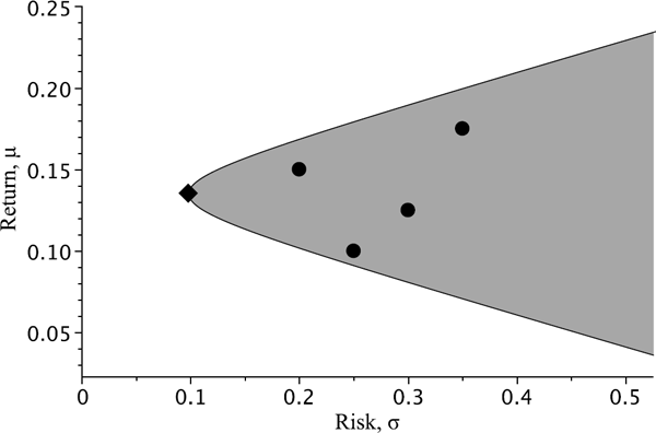
The set of admissible portfolios (the Markowitz bullet) in four underlying assets (which are marked by solid circles) bounded by the minimum variance line. The minimum variance portfolio is marked by a diamond.
Let us consider a portfolio in three underlying assets whose expected returns, standard deviations of returns, and correlations between returns are as follows:
μ1 = 0.1, |
σ1 = 0.2, |
ρ12 = ρ21 = −0.2, |
μ2 = 0.15, |
σ2 = 0.3, |
ρ23 = ρ32 = 0.2, |
μ3 = 0.3, |
σ3 = 0.4, |
ρ31 = ρ13 = −0.4. |
Solution. First, to apply the formulae in (3.28) and (3.32), we arrange the expected returns μi in a vector m and construct the covariance matrix C with entries Cij = σiσj ρij:
m=[0.100.150.30],C=[0.040−0.012−0.032−0.0120.0900.024−0.0320.0240.160].
The matrix C is positive definite, hence the inverse matrix C−1 exists:
C−1≅[30.30302.52525.68182.525211.7845−1.26265.6818−1.26267.5758].
The weights of the minimum variance portfolio are
wmv=uΤC−1uΤC−1u≅[0.60600.20530.1887]Τ.
The expected return μmv and standard deviation (the risk) of the return σmv of the minimum variance portfolio are
μmv=mΤwmv≅0.1480andσmv=√wΤmvCwmv≅0.1254.
To describe the minimum variance line, we need to find the weight vectors for two portfolios on the line. We found one of them—the minimum variance portfolio. Since μmv ≠ 0, the other portfolio on the minimum variance line to be selected can be a portfolio with zero expected return. To find its weights, apply E quation (3.32) where we put μ = 0 to obtain
w0=mΤC−1mDC−1u−mΤC−1uDC−1m≅[1.14590.4721−0.6180]Τ.
Now the portfolios with weights xwmv + (1 − x)w0, x ∊ ℝ, exhaust the minimum variance line.
Since w3 = 1 − w1 − w2, all portfolios in three basis assets from the above example can be described by the weights w1 and w2. On the (w1, w2)-plane, every portfolio line is represented by a straight line. For example, the line given by the equation w1 = 0 represents all portfolios in the basis assets 2 and 3 only; the line w1 + w2 = 1 represents all portfolios in the basis assets 1 and 2 only, etc. Figure 3.9 visualizes the set of admissible portfolios from Example 3.5 on the (w1,w2)-plane (the left plot) and on the (σ, μ)-plane (the right plot). The bold line represents the minimum variance line; the minimum variance portfolio is marked by a diamond.

The minimum variance line from Example 3.5 is plotted as a bold line. The minimum variance portfolio is marked by a diamond. The basis assets are represented by solid circles. The dashed lines represent portfolio lines.
3.3.4 Case without Short Selling
The case without short selling is very similar to that considered in the previous section. No short selling means that all positions in an investment portfolio have to be nonnegative. We can find the minimum variance portfolio line and the minimum variance portfolio by solving respective quadratic programming problems that have one additional condition: the weights wi are now nonnegative. To find the minimum variance portfolio, we need to solve (3.26):
f(w):=wΤCw→minw
subject to the constraints
uΤw=1,w≥0. (3.33)
Here, the meaning of w ≥ 0 is that all wi ≥ 0. To obtain a family of minimum variance portfolios parameterized by the expected return μ, we need to minimize f(w) subject to the constraints
uΤw=1,mΤw=μ,andw≥0. (3.34)
The constraints in (3.33) and (3.34) are almost the same as are in (3.27) and (3.29), respectively. The quadratic problems can be solved numerically. Computer systems such as MAPLETM, MATHEMATICATM, and MATLABTM can be applied to solve the minimization problems (3.26)–(3.33) and (3.26)–(3.34).
Let us consider the case with three assets from Example 3.5. The weights can be parameterized by two real variables w1,w2 ∊ [0, 1] with w1 + w2 ≤ 1 and hence w3 = 1 − w1 − w2 ≥ 0. On the (w1,w2)-plane, the set of admissible portfolios is represented by a triangle with vertices (0, 0), (0, 1), and (1, 0). Clearly, the expected return on a portfolio with nonnegative weights w is bounded above and below by max μi and min μi, respectively. Therefore, the minimum variance line is a bounded curve on the (σ, μ)-plane. It connects two points corresponding to the assets with the lowest μ and highest μ, respectively. The set of admissible portfolios (with nonnegative weights) is represented by a planar domain bounded by the minimum variance line and portfolio lines (without short selling) corresponding to different pairs of the underlying assets (see Figure 3.10).

3.3.5 Efficient Frontier and Capital Market Line
Given the choice between two risky assets, a rational investor will choose an asset with higher expected return μ and lower risk σ.
An asset with (μ1,σ1) is said to dominate another asset with (μ2,σ2) whenever μ1 ≥ μ2 and σ1 ≤ σ2. A portfolio in risky assets is called efficient if there is no other portfolio, except itself, that dominates it. The set of efficient portfolios among all attainable portfolios is called the efficient frontier.
In particular, an efficient portfolio has the highest expected return μ among all attainable portfolios with the same level of risk σ and has the lowest σ among all attainable portfolios with the same μ.
Let us consider the case with two risky assets. The set of admissible portfolios is represented by a portfolio line on the (σ, μ)-plane. The line is passing through the two base assets (σ1,μ2) and (σ2,μ2). As was proved in the previous section, there is a portfolio with the minimum possible variance σmv2 given in (3.13). For every σ>σmv, there are two portfolios on the portfolio line, (σ, μ1) and (σ, μ2), with μ1 <μ2. A rational investor would choose the portfolio (σ, μ2) with a higher expected return. Therefore, in the case of two risky assets, the efficient frontier is the upper half of the portfolio line with the minimum variance portfolio (σmv,μmv) as an endpoint. If one of the two assets is risk-free, then the portfolio line is a broken line with its vertex at the risk-free asset. The efficient frontier is the upper half-line. Both cases are represented in Figure 3.11.

In the situation with multiple risky assets (N > 2), the set of admissible portfolios (the Markowitz bullet) is a planar domain on the (σ, μ)-plane bounded by the minimum variance line. Fix the value of σ ≥ σmv and consider all admissible portfolios V with the standard deviation σV = σ. On the (σ, μ)-plane, this set is a segment enclosed by the minimum variance line. By maximizing the expected return, we find that the efficient portfolios are all lying on the upper half of the minimum variance line (see Figure 3.12a).

Finally, let us assume that one risk-free asset labelled B with the rate of return r is available in addition to N risky assets. Let 100α% of the capital be allocated in the risk-free asset and 100(1 − α)% is a risky portfolio:
rV=αr+(1−α)N∑i=1︸=:rℳwiri=αr+(1−α)rℳ,
where w1,...,wN are the allocation weights for the risky assets (so that w1 + ... + wN = 1 holds).
As is shown in Subsection 3.2.2, all portfolios with rV = αr + (1 − α)rℳ consisting of one risk-free and one risky asset (the risky portfolio Vℳ of an investment portfolio can be considered as a new asset) form a broken line having upper and lower half-lines with the common vertex at the point with coordinates (0,r). The efficient frontier constructed from such portfolios is the upper half-line like that in Figure 3.11. By taking a risky portfolio Vℳ anywhere in the Markowitz bullet, we can construct the set of admissible portfolios that is represented on the (σ, μ)-plane by a cone bounded by two half-lines, as is shown in Figure 3.13.

The set of admissible portfolios constructed from four risky assets and one risk-free asset.
The efficient frontier of the portfolios containing a risk-free asset in addition to N risky ones is the upper half-line which is passing through the point representing the risk-free asset and tangent to the minimum variance line. Indeed, to minimize the risk, the portfolio Vℳ in risky assets has to be selected on the minimum variance line. To maximize the return, the portfolio Vℳ has to be selected so that the upper half-line has the largest possible slope. If the risk-free return r is not too high, the largest possible slope is achieved when the upper half-line is tangent to the Markowitz bullet. If r is too high, then the efficient frontier is obtained in the limiting case as the portfolio Vℳ selected on the upper half of the minimum variance line goes to infinity. The efficient frontier is no longer tangent to the Markowitz bullet, but is parallel to its asymptote (recall that the shape of the bullet is a hyperbola). The tangency point with coordinates (σℳ,μℳ) is the so-called market portfolio. The efficient frontier is called the capital market line. Every rational investor forming her portfolio with a risk-free asset with return r and risky assets available on the market selects the portfolio on this line. Figure 3.12b shows the market line for portfolios with one risk-free and several risky assets.
The weights of the market portfolio are
wℳ=(mT−ruT)C−1uTC−1(m−ru).
The expected return, μℳ, and variance of return, σ2ℳ, of the market portfolio can be found by using (3.24) and (3.25). The capital market line that starts at the risk-free asset (represented by the point (0,r) on the (σ, μ)-plane) and passes through the market portfolio with expected return μM and standard deviation of return σℳ satisfies the equation
μ−rμℳ−r=σ−0σℳ−0⇔μ=r+μℳ−rσℳσ.
3.4 The Capital Asset Pricing Model
The Capital Asset Pricing Model (CAPM) attempts to relate ri, the return on asset i, to rM, the return of the entire market, which can be measured by some index such as Standard and Poor's index of 500 stocks (S&P500). In the Markowitz portfolio model, the market portfolio can be used as a good approximation to such a market index. Indeed, every rational investor will select a portfolio on the capital market line since it is the efficient frontier constructed from a risk-free asset and several risky assets. Therefore, every investor will be holding a portfolio with the same relative proportions of risky assets. This means that for each risky asset its weight in the market portfolio is equal to the relative share of the asset in the whole market.
The CAPM assumes that the dependence between ri and rℳ takes the following form:
ri=r+βi(rℳ−r)+∈i, (3.35)
where βi is a constant called the beta factor for asset i, r is a risk-free rate of return, and ∈i is a residual random variable having a normal distribution with mean zero. The residual ∈i is assumed to be independent of rℳ.
There are several ways to compute beta factors.
(1) Suppose that the joint probability distribution of ri and rℳ is given. Compute the covariance of ri and rℳ by employing (3.35) and using the independence of rℳ and ∈i:
Cov(ri,rℳ)=Cov(r,rℳ)︸=0+βiCov(rℳ,rℳ)︸=Var(rℳ)−βiCov(r,rℳ)︸=0+Cov(∈i,rℳ)︸=0=βiVar(rℳ).
Therefore, the beta factor of asset i is given by
βi=Cov(ri,rℳ)Var(rℳ). (3.36)
(2) Consider a market model with a set of market scenarios Ω. Suppose that for each market scenario ω ∊ Ω, the values of returns on asset i and the market portfolio ℳ are given. We can plot the value of ri(ωj) against rℳ(ω) for each ω ∊ Ω and then find the line of best fit, also known as the regression line. Employ the model ri = α + βrℳ + ∈i. So the residual random variable ∈i :Ω → ℝ is the difference between the actual return ri and the predicted return α + βrℳ. The line of best fit is defined by
E[∈2i]→minα,β.
The expected value of ∈2i is given by
E[∈2i]=E[r2i]−2βE[rirℳ]+β2E[r2ℳ]+α2−2αE[ri]+2αβE[rℳ].
A necessary condition for a minimum of E[∈2i] as a function of α and β is that the partial derivatives w.r.t. α and β should be zero at the point of minimum, (αi,βi):
∂∂αE[∈2i]=0⇔α+βE[rℳ]=E[ri],∂∂βE[∈2i]=0⇔αE[rℳ]+βE[r2ℳ]=E[rirℳ].
As a result, we obtain a system of linear equations that can be solved to find
βi=Cov(ri,rℳ)Var(rℳ),αi=E[ri]−βiE[rℳ].
Note that for the beta factor we obtained the same expression as that in (3.36).
(3) Suppose that historical data of returns on some portfolio V and the market portfolio M,{r(j)V,r(j)ℳ}j=1,2,...,N, are available. Let us find the line of best fit by minimizing the sum of squared residuals:
N∑j=1(r(j)V−(α+βr(j)ℳ))2→minα,β⋅
The solution to this minimization problem is
βi=N∑jr(j)Vr(j)ℳ−(∑jr(j)V)(∑jr(j)ℳ)N∑j(r(j)ℳ)2−(∑jr(j)ℳ)2,αi=∑jr(j)V−βi∑jr(j)ℳN.
The beta factors for individual assets can be computed by (3.36) or from historical data. The beta factor of a portfolio V in N assets with weights w1,...,wN is given by
βV=w1β1+⋅⋅⋅+wNβN.
Indeed, the covariance function is bilinear; therefore
βV=Cov(rV,rℳ)Var(rV)=Cov(w1r1+⋯+wnrN,rℳ)Var(rV)=w1Cov(r1,rℳ)+⋯+wNCov(rN,rℳ)Var(rV)=w1β1+⋯+wNβN.
Clearly, the beta factor of the market portfolio is equal to one.
By taking the mathematical expectation of both parts of (3.35), we obtain
μi=r+βi(μℳ−r),
where μi = E[ri] and μℳ = E[rℳ]. The expected return plotted against the beta factor of any portfolio will form a straight line on the (β, μ)-plane, called the asset market line.
3.5 Exercises
- Exercise 3.1. Show that the functions u1(x) = ln x and u2(x) = 1 − e−ax with a > 0 both satisfy the definition of a utility function, i.e., each of them is an increasing, concave function.
Exercise 3.2. Show that the functions u3(x) = xawith 0 <a < 1 and u4(x)= x − bx2 with b > 0 and x<12b both satisfy the definition of a utility function, i.e., each of them is an increasing, convex-upward function.
Exercise 3.3. An investor with capital W can invest an amount V = aW for some 0 ≤ a ≤ 1. If V is invested, then after one year the invested amount is doubled with probability p or lost with probability 1 − p. Suppose that the remaining capital W − aW can be put in a risk-free bank account to earn interest at an annual rate of interest r. How much should be invested by an investor using:
(a) a log utility function u(V) = ln V,
(b) an exponential utility function u(V) = 1 − e−0.1v?
Exercise 3.4. Consider an investment of $1000 in two risky assets whose returns follow a bivariate normal distribution with the following expected values and standard deviations:
μ1=0.1,σ1=0.2,μ2=0.15,σ1=0.3.
The correlation coefficient between the returns is ρ = −0.5.
(a) Suppose that the allocation weights of an investment portfolio for assets 1 and 2 are, respectively, w1 = x and w2 = 1 − x for some x ∊ ℝ. Show that the terminal value VT of a portfolio is normal. Find the expected value and variance of VT.
(b) Find the optimal portfolio when employing the utility function
u(V)=1−e−0.01V.
Exercise 3.5. Consider a market model with three scenarios {ω1,ω2,ω3} and two risky assets with returns r1 and r2. Let the probabilities of the scenarios and values of the returns be as follows:
ω
ℙ(ω)
r1(ω)
r2(ω)
ω1
0.5
10%
5%
ω2
0.3
5%
10%
ω3
0.2
15%
−5%
Find the expected values and standard deviations of the returns. Find the coefficient of correlation between r1 and r2.
Exercise 3.6. Show that the optimal allocation weights {wi} of one's investment portfolio Vt=∑Ni=1wiAit,t∈{0,T}, that correspond to amounts invested in each asset do not depend on the initial capital V0 when attempting to maximize the mathematical expectation of:
(a) a log utility function u(VT) = ln VT,
(b) a power utility function u(VT)=(VT)a with 0 < a < 1.
In other words, the maximization of E[u(VT)] reduces to the maximization of E[u(VTV0)].
Exercise 3.7. Plot portfolio lines with and without short selling for the case with two assets if
(a) |ρ12| = 1, μ1 = μ2, and σ1 ≠ σ2,
(b) |ρ12| = 1, μ1 ≠ μ2, and σ1 = σ2,
(c) μ1 = μ2, and σ1 = σ2.
Exercise 3.8. Consider three assets whose returns have the following standard deviation and correlation coefficients:
σ1=0.2,σ2=0.25,σ3=0.15,ρ12=−0.4,ρ13=0.3,ρ23=0.7.
Obtain the covariance matrix C.
- Exercise 3.9. Compute the weights in the minimum variance portfolio constructed using the assets in Exercise 3.7. Also compute the expected return and standard deviation of the minimum variance portfolio.
-
C = [10.75−0.30.7510.5−0.30.51]
cannot be a covariance matrix.
- Exercise 3.11. Suppose that the risk-free return is r = 3%. Find the weights in the market portfolio constructed from the three assets in Example 3.5. Compute the expected return and standard deviation of the return of the market portfolio.