
Replication and Pricing in the Binomial Tree Model
7.1 The Standard Binomial Tree Model
By combining the probabilistic framework in Chapter 6 with the main formal concepts of derivative asset pricing presented for the single-period model in Chapter 5, we are now ready to formally discuss derivative asset pricing within the multi-period binomial tree model. Let us begin by recalling the salient features of the standard T-period (recombining) binomial tree model on the space (Ω,ℙ,ℱ,F) with two assets, namely, a risky stock S and a risk-free asset B, such as a bank account or zero-coupon bond. The model is specified as follows.
- The time is discrete: t ∊ {0, 1, 2, ..., T}.
There are 2T possible market scenarios:
Ω≡ΩT={ω=ω1ω2⋯ωT:ωt∈{D,U},t=1,2,...,T},
where each scenario can be represented by a path in a multi-period recombining binomial tree.
- The set of events is the power set ℱ = 2Ω.
The probability function ℙ: ℱ → [0, 1] is given by
ℙ(E)=∑ω∈Eℙ(ω),E∈ℱ,whereℙ(ω)≡ℙ({ω})=p#U(ω)(1−p)#D(ω), (7.1)
and p ∊ (0, 1) is a probability of the event {ωt = U} = {ω ∊ Ω : ωt = U} for every t = 1, 2, ..., T.
The flow of information is described by the filtration F={ℱt}0≤t≤T, where ℱ0 = ∅ and ℱt is generated by the first t market moves ω1, ..., ωt for every t = 1, 2, ..., T, i.e., ℱt = σ(Pt), where the partition Pt is a collection of atoms of the form
Aω*1,ω*2,...,ω*t={ω∈Ω:ωn=ω*nforalln=1,2,...,t},ω*1,ω*2,...,ω*t∈{D,U}
(in particular, ℱT ≡ ℱ = 2Ω).
The stochastic stock price process, {St}0≤t≤T, which is adapted to the filtration F, is given by the recurrence
St(ω)=St−1(ω)u#U(ωt)d#D(ωt),t=1,2,...,T,
or, equivalently, by the relationship
St(ω)=S0uUt(ω)dDt(ω),t=0,1,2,...,T,
where Ut(ω) = #U(ω1, ω2, ..., ωt) and Dt(ω) = #D(ω1, ω2, ..., ωt) count, respectively, the number of downward and upward market moves; d and u are, respectively, downward and upward market movement factors which satisfy 0 < d < u; and ω ∊ ΩT is a market scenario. The initial price of the stock, S0 > 0, is known.
The deterministic price process, {Bt}0≤t≤T, for the risk-free asset is given by
Bt=B0(1+r)t,t=0,1,2,...,T,
where r > 0 is a one-period return. With loss of generality, we assume that we deal with a bank account such that B0 = 1. Note that for a unit zero-coupon bond paying $1 at time T, the initial value is B0 = (1 + r)−T.
Recall that a single-period binomial-tree model admits no (static) arbitrage portfolios in base assets iff there exists an equivalent martingale measure (EMM) ˜ℙ(g) for numéraire g ∊ {B, S}. An EMM ˜ℙ(g) is defined so that it is equivalent to the real-world measure ℙ (which is also called an actual or physical probability measure) and the base asset price processes discounted by g are ˜ℙ(g)-martingales. Let us extend this idea to the multi-period case. The probability function in (7.1) is specified by a single probability p = ℙ(U) of an upward move over a single period. The respective risk-neutral probability of an upward move, ˜p(g)=˜ℙ(g)(U), for either choice g = B or g = S, is
˜p≡˜p(B)=1+r−du−dor˜q≡˜p(S)=˜p⋅u1+r=1+r−du−d⋅u1+r.
In either case, the probability ˜p(g)∈(0,1) exists iff
d<1+r<u. (7.2)
By replacing in (7.1) the probability p by a risk-neutral probability ˜p(g), we can construct a risk-neutral probability measure ˜ℙ(g) defined on the σ-algebra ℱ = 2Ω. As is proved below, the base assets process discounted by numéraire g are ˜ℙ(g)-martingales. In other words, according to Definition 5.9, the probability measures ˜ℙ(B) and ˜ℙ(S) are equivalent martingale measures for the multi-period binomial model.
The discounted base asset price processes
{ˉSt:=Stgt}0≤t≤Tand{ˉBt:=Btgt}0≤t≤T
are ˜ℙ(g)-martingales for g ∊ {B, S}, i.e.,
˜E(g)t[ˉSt+1]=ˉStand˜E(g)t[ˉBt+1]=ˉBt
holds for all t = 0, 1, ..., T − 1, iff the condition (7.2) holds.
Proof. Let us consider the case with g = B (the other case is treated similarly). The discounted risk-free asset price process ˉBt is equal to 1 for all times t and hence the process ˉBt is a martingale. We now show that the process {ˉSt} is a martingale relative to ˜ℙ≡˜ℙ(B). Fix arbitrarily t ∊ {0, 1, ..., T − 1}. We have
˜Et[St+1Bt+1]=˜Et[Stu#U(ωt+1)d#D(ωt+1)(1+r)Bt]=StBt˜E[11+ru#U(ωt+1)d#D(ωt+1)]=StBt(u1+r˜p+d1+r(1−˜p)).
The last expression is equal to StBt and hence the martingale condition for the discounted stock price process is fulfilled iff ˜p=1+r−du−d. The condition ˜p∈(0,1) is equivalent to (7.2).
The EMM ˜ℙ(g) for g ∊ {B, S} exists iff (7.2) holds. Thus, according to the fundamental theorem of asset pricing (proved for the one-period case), there are no arbitrage portfolios iff d < 1 + r < u, i.e., the return on the risk-free asset is strictly between the downward and upward returns on the stock: d − 1 < r < u − 1. In the next sections, we will introduce the notion of an arbitrage portfolio strategy and will prove the fundamental theorems in the multi-period case. Apparently, the condition (7.2) guarantees the absence of arbitrage strategy in the binomial tree model as well.
7.2 Self-Financing Strategies and Their Value Processes
Consider an investor who begins with an initial capital to be invested in base securities. Suppose that injecting or withdrawing funds is not allowed in the future time, although the investor can modify the investment portfolio by changing the positions in base assets. For example, the investor may sell some stock shares and invest the proceeds without risk. As a result, a sequence of investment portfolios in the base assets indexed by time is constructed. Recall from Section 2.2.4 in Chapter 2 that such a sequence of portfolios that does not allow for injecting or withdrawing funds is called a self-financing strategy. A self-financing strategy allows the investor to create a portfolio with a target probability distribution or hedge a cash flow during a period of time. Self-financing strategies are important for the no-arbitrage pricing of derivative securities when combined with replication in the multi-period setting where trading (i.e., portfolio re-balancing) in the base assets is allowed at times t = 0, 1, ..., T. The simplest example of a self-financing strategy is a static portfolio in the base assets that does not change in time.
For the binomial model there are only two base assets, namely, a risky stock S and a risk-free bank account B. Thus, any investment (or trading) strategy Φ is a sequence of portfolios in the two base assets:
Φ={φt}0≤t≤T−1,whereφt=(βt,Δt).
Throughout we shall use βt and Δt to denote the respective positions in assets B and S at time t. For each t = 0, 1, ..., T − 1, the portfolio φt is formed at time t and held until time t + 1, i.e., φt = (βt, Δt) is the portfolio held in the time period [t, t + 1). At time t + 1 the investor can re-balance the portfolio to form the new portfolio φt + 1 = (βt + 1, Δt + 1), which is held in the time period [t +1, t + 2), and so on. At each trading time, we will insist that the re-balancing of the positions must satisfy the self-financing condition.
Let us begin with time t = 0. The investor begins with a given initial capital or wealth Π0 which completely finances the initial portfolio with positions φ0 = (β0, Δ0) in the base securities, i.e., with acquisition value
∏0=∏0[φ0]:=Δ0S0+β0B0.
We use the notation Πt[φ] to denote the time-t value of a portfolio φ = (β, Δ) in the base assets B and S:
∏t[φ]≡∏t[(β,Δ)]:=ΔSt+βBt.
By the above self-financing of the initial portfolio, the initial position Δ0 in the stock determines the initial investment in the risk-free asset:
β0=∏0−Δ0S0B0⇒∏0=Δ0S0+(∏0−Δ0S0B0)B0.
The investor holds this portfolio until a time just prior to time t = 1, and at time t = 1 the investor liquidates it to form a new one. The liquidation value is the value of the portfolio with the positions being those at time 0 but with the prices of the base assets being those at the present time t = 1:
∏1:=∏1[φ0]=Δ0S1+β0B1=Δ0S1+(∏0−Δ0S0)B1B0=Δ0S1+(∏0−Δ0S0)(1+r).
These proceeds are used entirely to finance the formation of a new portfolio φ1 = (β1, Δ1) with the same acquisition value Π1 = Π1[φ1] = Δ1S1 + β1B1. This is the self-financing condition applied at time t = 1, giving
β1=∏1−Δ1S1B1⇒∏1=Δ1S1+(∏1−Δ1S1B1)B1.
The position Δ1 is determined based on the information available at time 1, i.e., Δ1 = Δ1(ω1). By repeating the same procedure at every time step, we obtain general formulae for the equivalent liquidation and acquisition values Πt, t = 1, ..., T, for any self-financing strategy:
∏t:=∏t[φt−1]=Δt−1St+(∏t−1−Δt−1St−1)(1+r), (7.3)
where φt = (βt, Δt) is a portfolio in the base assets B and S formed at time t = 0, 1, ..., T − 1. Since the liquidation value and the acquisition value of a self-financing strategy are the same at every date t ≥ 0, we will only speak of the value Πt of a self-financing strategy.
At every time step t ≥ 0, the positions Δt and βt are determined based on the market information available at time t. In other words, Δt and βt depend on the first t market moves and we express this as
Therefore, the portfolio process {φt}0≤t≤T − 1 is adapted to the natural filtration , i.e. Δt and βt are ℱt-measurable random variables for all t ≥ 0.
Clearly, any self-financing strategy in the binomial tree model is fully described by the process {Δt}0≤t≤T − 1 of stock positions (i.e., the delta positions) and the initial value Π0. The positions βt can be calculated with the use of the self-financing condition:
Since the delta process is adapted to the natural filtration , the value process is expected to be adapted to , as is proved in the next proposition.
Let {Δt}0≤t≤T − 1 be a process adapted to the natural filtration of a binomial tree model, and let Π0 be the initial known capital. Then the value process {Πt}0≤t≤T defined recursively by the wealth equation
is adapted to the natural filtration as well, i.e., Πt = Πt(ω1ω2 ... ωt) for all 0 ≤ t ≤ T.
Proof. Let us prove the assertion by induction. The initial value Π0 is an ℱ0-measurable constant. For any 1 ≤ t ≤ T, the value Πt = Δt−1St + (Πt−1 − Δt−1St−1)(1 + r) is ℱt-measurable since Πt is a linear combination of ℱt-measurable variables St, St−1, and Πt−1. The latter is measurable w.r.t. ℱt−1 ⊂ ℱt.
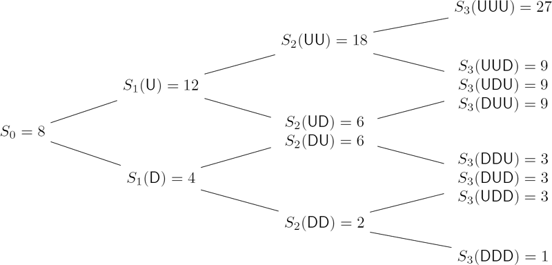
Consider a three-period recombining binomial tree model with S0 = 8, B0 = 1, , , and . Find the terminal value of a self-financing strategy with the initial value Π0 = 10 and stock positions Δt given as the number of upward moves in the first t market movements for each t = 0, 1, 2.
Solution. The recombining binomial tree for the stock price process is given in Figure 7.1. Now construct the self-financing strategy and calculate its value step by step going forward in time. Note that the positions Δ0 = 0, Δ1 = #U(ω1), Δ2 = #U(ω1ω2) are ℱ0-, ℱ1-, and ℱ2-measurable, respectively. The self-financing investment strategy is therefore adapted to the natural filtration. Construct the strategy for each t = 0, 1, 2 as follows.
t = 0: Since Δ0 = 0, at time 0 all the capital is invested in the bank account with .
t = 1: There are no shares of stock in our investment portfolio so far. Therefore, its value is independent of ω1 and by the above wealth equation:
If ω1 = D, Δ1(D) = 0 and β1(D) = 10. If ω1 = U, then Δ1(U) = 1 and
t = 2: The self-financed portfolio has value Π2(ω1ω2) = β1(ω1)B2 + Δ1(ω1)S2(ω1ω2) for each of four scenarios: ω1ω2 ∊ {DD, DU, UD, UU}. Let us calculate the respective liquidation values of Δ2 and β2 in each case.
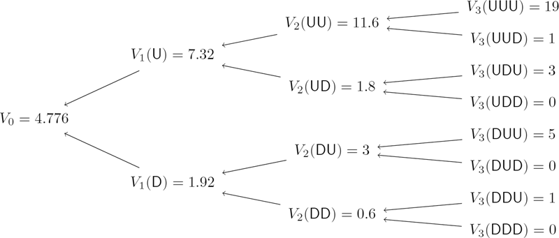
The terminal value Π3 of the strategy is calculated by
The full details of this three-period strategy, for every scenario, are summarized in Figure 7.2.

7.2.1 Equivalent Martingale Measures for the Binomial Model
As mentioned at the start of this chapter, we fix the filtration to be the one generated by the market moves (i.e., the scenarios in the binomial tree); hence, the filtration also corresponds to the natural filtration generated by the stock price process. Since our main interest is in pricing derivative assets, the martingale property will be relevant under risk-neutral probability measures. We already referred to these measures as so-called equivalent martingale measures (EMMs). In the next chapter we shall define an EMM for the general case of N basic securities within the multi-period setting. At this point we need only to deal with the binomial multi-period model with two basic securities: the risk-free bank account B (or money market account, or zero-coupon bond) and the risky stock S. Hence, given a numéraire asset g, a corresponding EMM is defined such that the discounted value processes of the risk-free asset and the stock are both -martingales (see Theorem 7.1).
Recall Chapter 5, where we proved that for a single-period (Arrow–Debreu) model the value process of any static portfolio in the base securities, discounted by a numéraire asset g ∊ {B, S}, is a -martingale, i.e., the discounted portfolio value process is a martingale under the measure . We are now ready to extend such a result for the binomial tree model to the multi-period setting in the case of dynamic self-financing portfolio strategies.
Suppose that an equivalent martingale measure for a numéraire asset g (e.g., the bank account B or stock S) exists. Let {Δt}0≤t≤T − 1 be a process adapted to the natural filtration of the binomial tree model. Let {Πt}0≤t≤T be generated recursively by the wealth equation (7.6). Then the value process discounted by g, , is -martingale.
Proof. Note that, for every 0 ≤ t ≤ T, the value is clearly ℱt-measurable and integrable, i.e., . It then suffices to prove the single-step martingale expectation property under the -measure: , for every 0 ≤ t ≤ T − 1. We now use the fact that the discounted stock price and risk-free asset price processes, and , are -martingales and that Δt, , , are ℱt-measurable. From the wealth equation (7.6) with Bt+1/Bt = 1 + r we have:
Hence, the process is a -martingale.
Suppose that the interest rate r is fixed and that the risk-free bank account (or zero-coupon bond) is used as numéraire. Then we obtain the following well-known result for the risk-neutral expectation (and risk-neutral growth rate) of the self-financing portfolio value process.
Corollary 7.4.
Let be the EMM for the numéraire g = B, i.e., and since Bt + 1 = (1 + r)Bt for all t ≤ 0. Then,
and hence for all t ≥ 0.
Verify that the self-financed portfolio value process in Example 7.1, discounted by the risk-free asset price process, is a martingale under the measure .
Solution. The risk-neutral probabilities for the up and down moves are
It is sufficient to verify that for t = 0, 1, 2.
Another corollary of Theorem 7.3 is the first fundamental theorem of asset pricing (FTAP). It states that there are no arbitrage opportunities iff there exists an EMM for a numéraire g. So far, such an assertion has been proved for static portfolios in the one-period or multi-period setting. However, one can create an arbitrage opportunity by manipulating with a portfolio in base assets without injecting or withdrawing funds. In other words, a specially constructed self-financing strategy can be an arbitrage. Let us prove that there are no self-financing arbitrage strategies in a binomial tree model iff there exists an EMM. First, we need to have a formal definition of an arbitrage in a multi-period trading model as follows.
An arbitrage strategy in a multi-period model is a self-financing strategy with nonnegative value process and zero initial value Π0 such that P(Πt > 0) > 0 holds at some time t ∊ {1, 2, ..., T}.
Suppose that a binomial tree model admits no arbitrage. In particular, there are no static (i.e., with constant positions in base assets as in any single-period setting) arbitrage portfolios. Then, as was proved before, there exists an EMM. To complete the proof of the FTAP for the binomial tree model we only need to prove the following converse statement.
Suppose that an EMM for a numéraire g exists. Then there are no self-financing arbitrage strategies.
Proof. Suppose that a self-financed arbitrage strategy with initial value zero and delta positions {Δt}t≥0 exists. The value process for such a strategy must satisfy the wealth equation in (7.6) such that (by the arbitrage assumption) Πt(ω) ≥ 0 for all ω ∊ Ω and t ≥ 0. Moreover, arbitrage implies that there exists a time m ∊ {1, 2, ..., T} and market scenario ω* ∊ Ω such that Πm(ω*) > 0. Therefore,
This contradicts Theorem 7.3, since .
7.3 Dynamic Replication in the Binomial Tree Model
7.3.1 Dynamic Replication of Payoffs
A key idea in modern finance is the replication of a financial claim with the use of portfolios in other (base) assets. The two most important applications of replication is the no-arbitrage pricing of derivative securities and hedging their liabilities. Consider a derivative security with maturity at time T and payoff function X : ΩT → ℝ. Recall that ℒ(ΩT) denotes the collection of all payoff functions on the sample space ΩT. The structure of a payoff can be quite general. It can depend on the whole path ω, or on a quantity calculated along the stock price path such as an average of the stock prices over some time window, or only on the terminal stock price ST. For example, the payoff of a non-path-dependent derivative, such as a standard European call or put option, with exercise only at maturity T, is a function of only the terminal stock price ST and is given by X(ω) = Λ(ST (ω)) with function Λ : ℝ+ → ℝ, where ℝ+ := [0, ∞). Hence, in what follows we allow for generally path-dependent payoffs where the random variable X is ℱT-measurable, i.e., the payoff is determined by possibly the entire sequence of market moves ω ≡ ω1 ... ωT ∊ ΩT.
Let {Vt}0≤t≤T denote the price process of the derivative security, i.e., Vt is the price of the derivative security at time t. At maturity time, the derivative price is given by the payoff function VT = X, where X : ΩT → ℝ. The writer of a derivative needs to calculate the no-arbitrage current price, V0, of the contract. As we saw in great detail in Chapters 2 and 5, in the single-period model, the price of a derivative security must equal the initial value of a portfolio replicating the derivative payoff at maturity. In the multi-period setting, such a replication can only be done dynamically with the use of self-financing strategies. It is possible to construct such a strategy that replicates the whole derivative price process from time 0 until maturity T. Knowledge of the derivative price process is required for hedging the writer's liabilities.
A self-financing strategy {φt}0≤t≤T − 1 is said to replicate the payoff X at maturity T if its value at maturity T, given by ΠT = ΠT [φT −1], equals the payoff value for all possible scenarios, i.e.,
According to the law of one price, the initial value Π0 of a strategy that replicates the payoff X of a derivative maturing at time T must equal the initial value V0 of the derivative, or else an arbitrage opportunity exists. Moreover, we shall prove that in the absence of arbitrage opportunities, the price of the derivative, Vt is equal to the value Πt ≡ Πt[φt] of the replicating strategy at every time t.
To construct a self-financing strategy that replicates a derivative with payoff X, we proceed as follows. First, we construct a no-arbitrage derivative price process {Vt}0≤t≤T recursively backward in time starting from maturity time T. Second, we obtain a sequence of (delta) positions in the stock, {Δt}0≤t≤T − 1, corresponding to the price process. Finally, we show that the process {Δt} is nothing more than a replicating strategy for the derivative price process so that the value process {Πt}0≤t≤T generated by the strategy coincides with the derivative price process at all intermediate dates and at maturity, i.e., Πt(ω) = Vt(ω) for all 0 ≤ t ≤ T and all scenarios ω ∊ Ω. Note that ΠT (ω) = VT(ω) = X(ω) holds at maturity by the definition of a replicating strategy. Before we prove a general result, let us study how this procedure works for the simple one-and two-period cases.
(The cases with T = 1 and T = 2). Assume that the binomial tree model admits no-arbitrage, i.e. d < 1 + r < u holds. Let be the usual risk-neutral measure (for the numéraire asset g = B). Construct the replicating strategy and find the no-arbitrage prices for an arbitrary derivative with maturity time (a) T = 1 and (b) T = 2.
Solution.
Case with T = 1. In the one-period case, the replicating portfolio is static and formed at time 0, as we already saw in Chapter 2. The initial value Π0 is invested in Δ0 shares of stock, leaving us with the risk-free asset position with value Π0 − Δ0S0. At time 1, the portfolio value is Π1(ω) = Δ0S1(ω) + (Π0 − Δ0S0)(1 + r). Let us choose Π0 = V0 and Δ0 such that Π1(ω) = V1(ω) for ω ∊ Ω1 = {D, U}. Since there are two possibilities for ω1, we obtain the linear system of two equations in two unknowns Δ0 and V0:
This system has a unique solution with Δ0 obtained by simply subtracting the first and second equations in (7.7):
Substituting this expression for Δ0 into either of the equations in (7.7) gives the current price of the derivative in terms of known (payoff) values V1(U) and V1(D):
Note that the last expression corresponds to the discounted expected value of the derivative payoff with risk-neutral probabilities with asset B as numéraire:
Case with T = 2. Let us construct a replicating strategy {Δt}t = 0, 1 with the time-2 value satisfying Π2(ω) = V2(ω) for all ω ∊ Ω2 = {DD, DU, UD, UU}. At time 0, the strategy is already specified above, i.e., take a position Δ0 in shares of stock and a position in the risk-free bank account with value Π0 − Δ0S0. This gives Δ0 and V0, respectively, as in (7.8) and (7.9). At time 1, we liquidate the old portfolio and form a new portfolio having value Π1(ω1) = V1(ω1) and with new position Δ1(ω1) in the stock for any given market scenario with first move ω1. At time 2, the value of this new portfolio, as given by the wealth equation for t = 2, becomes
By replication, Π2(ω1ω2) must equal V2(ω1ω2) for all four possible market scenarios ω1ω2. Hence, we obtain a system of four linear equations which are grouped into two pairs of equations. The first pair (for ω1 = U) gives two equations in two unknowns Δ1(U), V1(U):
and the second pair (for ω1 = D) in the two unknowns Δ1(D), V1(D):
At this point it is important to observe that both of these pairs of equations are of the same form as (7.7) and hence are solved in the same manner. In particular, solving (7.10) gives
and
Similarly, solving (7.11) gives
and
Combining both expressions for the derivative prices at t = 1 gives
We hence see from this last equation, and Equation (7.9), that the derivative prices at times t = 0 and t = 1 are given by the discounted (risk-neutral) expected value of the derivative price at time t + 1. Hence, by the tower property, the initial price of the derivative is expressible as an expectation of the payoff at time t = T = 2, discounted back by two periods:
Now, we consider the general case for any finite number of T ≥ 1 periods. Assume the absence of arbitrage opportunities. Let us define recursively backward in time the price process {Vt}0≤t≤T of a derivative with maturity time T and given payoff function X ∊ ℒ(ΩT). Fix arbitrarily time t ∊ {0, 1, ..., T − 1} and market moves ω1, ω2, ..., ωt ∊ {D, U}. The stock price St+1 conditional on ω1, ω2, ..., ωt follows a binomial single-period sub-tree: St+1 = Stu or St+1 = Std if ωt+1 = U or ωt+1 = D, respectively. Applying the single-step discounted expectation formula (e.g., as in Equation (7.9)) to the sub-tree originated at St(ω1ω2 ... ωt) gives
where and are risk-neutral probabilities given above. At maturity, we set
Define the strategy {Δt}0≤t≤T − 1 as follows:
Now, let us prove that the derivative price process {Vt}0≤t≤T and the value process for the self-financing strategy {Δt}0≤t≤T − 1 have the same value at all times t = 0, 1, ..., T, i.e., the portfolio value process with (delta hedging) strategy {Δt}0≤t≤T − 1 replicates the derivative price process.
Consider a derivative security with ℱT-measurable payoff X, at maturity T. Define the derivative price process {Vt}0≤t≤T by (7.16)–(7.18) and the self-financing portfolio strategy {Δt}0≤t≤T − 1 by (7.19). Set Π0 = V0 and construct recursively forward in time the value process {Πt}0≤t≤T via the wealth equation (7.6). Then, the strategy replicates the derivative price process at every time, i.e.
holds for all t = 0, 1, ..., T and all market moves ω1, ω2, ..., ωt ∊ {D, U}.
Proof. We prove the assertion by induction. For t = 0, the equality Π0 = V0 follows trivially by the definition of the initial price. Now assume that (7.20) holds for some time t and show that it holds for time t + 1. Fix an arbitrary sequence of moves ω1ω2 ... ωt. By the induction assumption, Πt(ω1ω2 ... ωt) = Vt(ω1ω2 ... ωt), and since ωt+1 = U or D, we need to prove that
Let us only consider the case with ωt+1 = D and St+1 = Std, since the case with ωt+1 = U is treated similarly. The wealth equation (7.6) then gives
where Δt is given by (7.19):
Substituting this into (7.21), cancelling out St, and using and Πt = Vt gives
(and by using Equation (7.16))
Remarks.
Applying the tower property of conditional expectations to (7.17) gives us the (multistep ahead) risk-neutral pricing formula for any derivative with payoff VT = X ∊ ℒ(Ω) at maturity T:
or, in short,
In particular, the initial derivative price is
- Theorem 7.6 is a particular case of a more general result presented below in Section 7.3.2, where here we take Xt = 0 for all t = 0, 1, ..., T − 1 and XT = X ≠ 0, i.e., the derivative has a payoff (i.e., a cash flow) only at maturity T.
A corollary of Theorems 7.3 and 7.6 is the property that, in the measure where g ∊ {B, S}, the discounted derivative price process is a martingale:
Note that this is consistent with the fact that, within the measure , the growth rate of the portfolio value is given by the interest rate, i.e., Bt = (1 + r)t−s Bs gives .
Theorem 7.6 can be generalized to the case with an arbitrary numéraire asset g. Equation (7.17) is rewritten as follows:
or, equivalently,
where denotes the expectation conditional on ℱt and w.r.t. the risk-neutral probability measure . Applying the tower property to (7.26) gives
That is, the time-t derivative price Vt discounted by the numéraire gt is given by the mathematical expectation (in the risk-neutral measure ) of the discounted payoff VT/gT. Note how this more general result recovers Equation (7.22) when we choose the bank account as numéraire, i.e., when gt = Bt we obtain the usual discount factor .
In a model with a finite number of states, the conditional mathematical expectation in (7.22) or (7.27) can be calculated as a sum over ω ∊ Ω. In particular, (7.22) can be written using Equation (6.33) of Chapter 6 where t = n, T = N, and X ≡ VT:
where and ω = ω1 ... ωT, 0 ≤ t ≤ T. If, instead, we choose the stock as numéraire, i.e., gt = St, then (7.27) gives us yet another equivalent formula for the derivative price:
where now .
In summary, we have derived two methods for calculating derivative prices. The first method involves the use of a single-step recurrence formula as in (7.16) or (7.26), which is used to calculate the prices one by one recursively backward in time. The second method employs a multi-step pricing formulas as in (7.27), (7.28), or (7.29). It allows us to calculate the derivative price at any intermediate date by averaging the values of the payoff function weighted by the risk-neutral probabilities of all the (T − t)-step paths ωt+1 ... ωT.
The replicating strategy {Δt}t≤0 is also called a delta hedging strategy. It allows the writer of a derivative contract to hedge perfectly the contract until the expiration date. Suppose that the writer sells one derivative contract for V0 dollars and uses the proceeds to form a replicating portfolio, (β0, Δ0), in the bank account and the stock. As a result, the total value of the investment portfolio of one short derivative, Δ0 shares of stock, and β0 units of the risk-free asset is zero. At the end of each period, the investor changes (i.e., re-adjusts) the positions in the stock using (7.19) and (7.5). According to Theorem 7.6, the total value of the portfolio remains equal to zero. At maturity, the investor closes the positions in the stock and bank account to pay out the premium (if any) to the holder of the derivative contract. The proceeds cover the payoff in full. The whole situation is a zero sum game without any risk involved.
The next question arising naturally is whether the binomial tree model is complete, that is, every claim can be replicated. Recall that a single-period model is said to be complete if every payoff can be replicated by a portfolio in base assets.
A multi-period model is said to be complete if every ℱT-measurable payoff X : ΩT → ℝ can be replicated by a self-financing trading strategy in base assets.
Theorem 7.6 states that every payoff can be replicated by a self-financing strategy. Thus, the binomial tree model is indeed complete. To illustrate this important result, we will find the price process and replication strategy for a path-dependent derivative in the following example.
Consider a binomial tree model from Example 7.1. Determine the prices and replicating strategy for a lookback call option with payoff
Solution. First, we shall construct a tree of possible scenarios. To calculate the payoff function at maturity T = 3 we need to know the minimum price
for all market scenarios ω ∊ Ω3. The sampled minimum mt = min0≤n≤t Sn, t = 0, 1, 2, 3, can be calculated simultaneously with stock prices using the formula mt = min{mt−1, St}, t = 1, 2, 3, where m0 = S0. Since the value of mt depends on the historical path of the stock price process (i.e., a market scenario ω), the result can be represented using a nonrecombining scenario tree, as given in Figure 7.3. As is clearly seen from Figure 7.3, the tree cannot be reduced to a recombining one since m2(DU) ≠ m2(UD), m3(UUD) ≠ m3(UDU) ≠ m3(DUU), etc.

A binomial tree with stock prices S and sampled minimum values m calculated for each node. There are |Ω3| = 8 distinct paths from time 0 to 3.
To calculate the derivative prices Vt, t = 0, 1, 2, we first evaluate the payoff function
for all eight possible scenarios ω ∊ Ω3. After that, using the backward recursion (7.16) with and , we compute derivative prices as follows:
where ω1, ω2 ∊ {D, U}. The results of our computations are summarized in Figure 7.4.
A scenario tree with derivative prices calculated for each node of a three-period nonrecombining tree.
We can now also obtain the replicating strategy using the delta hedging formula in (7.19) for Δt, t = 0, 1, 2:
The alternative method for computing the derivative prices is to use (7.28). For example, the initial price can be computed by the following discounted expectation:
7.3.2 Replication and Valuation of Random Cash Flows
Consider a financial contract whose payoff is spread over all T periods. Let the time-t payment be Xt for all t ∊ {0, 1, ..., T}. In general Xt is an ℱt-measurable random variable. In other words, Xt is a function of the first t market moves ω1, ω2, ..., ωt. So we deal with a stream of random cash flows {Xt}0≤t≤T adapted to the filtration . We allow these payments to be negative as well as positive. If a payment is positive (negative), then the holder, who is long on the contract, receives (makes) the payment.
Such a stream of cash flows can be replicated by a self-financing strategy in the base securities S and B. Start with the capital Π0 = V0. At time t = 0, we make the payment X0 and form a portfolio (β0, Δ0) with the total cost of Π0 − X0. At time t = 1 its value is
At every time t ∊ {1, ..., T}, we liquidate the portfolio (βt−1, Δt−1) whose total value (before the payment Xt is made) is governed by the following wealth equation:
Consider a derivative security with the payoff process {Xt}0≤t≤T adapted to the filtration . Define the derivative price process {Vt}0≤t≤T by the following backward-in-time recursion:
and the strategy {Δt}0≤t≤T − 1 by (7.19). Then the value process {Πt}0≤t≤T given by the wealth equation (7.30) coincides with the derivative price process:
for all 0 ≤ t ≤ T and all ω1, ω2, ..., ωt ∊ {D, U}. In other words, {Δt}0≤t≤T − 1 is a replicating strategy for the derivative security with the payoff process {Xt}0≤t≤T.
Proof. The proof is analogous to that of Theorem 7.6 and is left as an exercise for the reader.
Equation (7.32) can be written in a compact form using the risk-neutral mathematical expectation:
Applying this formula successively and using the tower property gives
In other words, the value Vt of the stream of cash flows at time t is given by the sum of the time-t risk-neutral values of all present and future payments. Here, we assume the risk-neutral measure .
7.4 Pricing and Hedging Non-Path-Dependent Derivatives
Equation (7.28) allows us to calculate the current derivative price by averaging the discounted payoff values calculated for all market scenarios. However, it is time and memory consuming to tabulate the payoff function for 2T scenarios. For example, a naive implementation of (7.28) for a 100-period binomial tree leads to a large amount of computation with 2100 ≅ 1.268 × 1030 market scenarios!
We know that in a recombining binomial tree many market scenarios lead to the same prices of S. For example, there are only T + 1 different time-T stock prices: ST = S0undT − 1 for n = 0, 1, ..., T. Consider a non-path-dependent derivative. At maturity, the payoff is a function of the stock price, X = Λ(ST) (recall that Λ is used here to denote a known payoff function of the price ST of the underlying asset). Thus, we expect that the derivative price is a function of the spot price for any time t preceding the maturity: Vt = Vt(St). The number of possible values of St is t + 1, which is significantly less than 2t. Therefore, we may organize the computation in a more efficient manner by computing derivative values on the recombining binomial tree.
To prove that the time-t derivative price Vt is only a function of the current spot St, we use the Markov property of the stock price process within the risk-neutral expectation pricing formula. Recall the definition of a discrete-time Markov process from Chapter 6. From the tower property, we have that if the Markov property holds for one period of time then it holds for any multiple time periods. Clearly the stock price process {St}t≥0 is a Markov process since, given any (Borel) function g,
[Note that the Markov property holds in any equivalent probability measure.] Therefore, from the multi-step Markov property of the stock price process applied to the risk-neutral expectation of the discounted payoff function Λ(ST), the time-t derivative price must be given by a function of t, St, say f(t, St):
This is an equation stating the equivalence of two random variables. On any given ω ∊ Ω we have Vt(ω) = f(t, St(ω)). Given a numerical value S for the stock price for a given outcome ω, i.e., St(ω) = S, then the derivative price function f(t, S) is an ordinary function of ordinary variables t, S. Note that below we shall also write Vt(S) to denote the time-t derivative price for St = S.
The possible values of S correspond to the nodes of the binomial tree and the derivative value can be calculated recursively backward in time on all these nodes:
and VT(ST, n) ≡ Λ(ST, n), where St, n : = S0undt − 1 for all n = 0, 1, ..., t and t = 0, 1, ..., T. Hence, this recovers the backward recurrence formula in Equation (4.12) of Chapter 4.
On the other hand, we can derive a direct formula for Vt(S) at t = 0, 1, ..., T − 1, given as the discounted mathematical expectation of the payoff function. Applying (7.22) to a European-style derivative with payoff Λ(ST) gives
The price St is ℱt-measurable. The ratio is independent of ℱt, since it is a function of ωt+1, ..., ωT, i.e. for all ω = ω1 ... ωT we have
Here, HT −t(ω) := #U(ωt+1, ..., ωT) = UT(ω) − Ut(ω), where Ut is defined in Equation (6.3) of Chapter 6. The variable HT −t counts the number of upward moves in the sequence ωt+1, ..., ωT. Hence, under . The random variable HT −t is independent of ℱt; the variable St is ℱt-measurable. Therefore, by using Proposition 6.7, we obtain
As is seen from the above equation, Vt is a function of St. By setting t = 0, we can recover the risk-neutral pricing formula (4.13) from Chapter 4 for the initial price V0 of a European-style derivative.
Using (7.34), we can compute derivative prices for each node of the recombining binomial tree. As a result, we obtain the derivative pricing function, Vt(S),, which is a function of calendar (actual) time t ≤ 0 and stock price (spot) S > 0. It is defined for every node of the binomial tree and hence can be represented in a tree form as well (see Figure 7.5).

A recombining binomial tree with stock prices S, derivative prices V, and replication stock positions Δ given for each node.
The stock positions of the replication strategy {Δt}0≤t≤T − 1 given by (7.19) are functions of derivative and stock prices. Therefore, the position Δt does not explicitly depend on ω1, ..., ωt, but it is a function of only St = St(ω1, ..., ωt) and given by
Equation (7.5) takes the following form:
Hence the computation of the replication strategy reduces to the calculation of stock positions for each node of the recombining binomial tree. As a result we obtain a binomial tree where three quantities are computed for each node (t, n), where t = 0, 1, ..., T and n = 0, 1, ..., t: the stock price St, n : = S0undt−n, the derivative price Vt, n := Vt(St, n), and the replication position Δt,n : = Δt(St, n) (see Figure 7.5).
The recurrence formulae (7.34) and (7.37) can now be written in a more compact form:
The terminal condition is VT,n = Λ(ST, n) for 0 ≤ n ≤ T.
Consider the three-period recombining binomial tree model from Example 7.1 with S0 = 8, B0 = 1, , , and . Determine the option prices and replication strategy for a standard European call with maturity time T = 3 and strike price K = 8 (i.e., the call option is at the money).
Solution. We first calculate the payoff values and then the call option prices Ct(St, n) at t = 0, 1, 2 using the backward-in-time recursion (7.34), which takes the following form:
where St, n = S0undt−n = 8 · 1.5n · 0.5t−n for n = 0, 1, ..., t.
t = 3: At maturity T = 3, calculate the payoff values C3(S3) = (S3 − 8)+, where S3 ∊ {1, 3, 9, 27}:
t = 2: Calculate the option prices at time t = 2:
t = 1: Calculate the option prices at time t = 1:
t = 0: The initial option price is
Now, compute the replication strategy {(βt, Δt)}t = 0,1,2 using the formulae (7.37) and (7.38):
The results are summarized in Figure 7.6.

Call option prices and replication portfolio positions β and Δ calculated for each node of the recombining binomial tree.
7.5 Pricing Formulae for Standard European Options
The formula (7.36) allows us to price any non-path-dependent derivative with a given payoff function Λ including nonlinear functions of the stock price. However, the option price formula (7.36) can be written in a simpler form for the standard European call and put payoff functions. In Chapter 4 we present the binomial pricing formulae (4.17) and (4.18) for initial (time-0) prices of the European call and put options. Those formulae are given in terms of the binomial CDF B. Let us generalize that result and derive a closedform formula of the time-t derivative price (with arbitrary t) for a class of derivatives with piecewise linear payoffs.
According to the pricing formula (7.35), the derivative price is given by the risk-neutral expectation of the payoff function. First, we observe that the European call, put, and chooser option payoffs, which are, respectively, given by (S − K)+, (K − S)+, and S ∧ K, can be represented as a linear combination of functions from the list
Indeed, the call and put payoffs admit the following respective representations:
Using the linearity of the mathematical expectation in (7.35) and the martingale property for the discounted stock price process gives the following formulae for time-t prices of the standard European call and put options:
As is seen, the evaluation of European call and put options reduces to computation of the conditional expectations and . The expectation of the indicator function, , is equal to the conditional probability of the event {ST ≤ K}:
Recall that the ratio ST/St can be expressed in terms of a binomial random variable:
where is independent of St. Dividing both parts of the inequality ST ≤ K by St and using (7.42) allows for reducing the event {ST ≤ K} to an equivalent event for the binomial random variable HT −t:
where mT − t(St) ≡ m(K, St, u, d, T − t) is given by
Here we assume that the strike price K lies in the interval [StdT − t, StuT − t], which includes all possible stock prices ST conditional on St. If K < StdT − t holds, i.e., the strike price is less than the minimum value of ST conditional on St, then we set mT − t = −∞. If K >StuT − t holds, i.e., the strike price is greater than the maximum value of ST conditional on St, then we set mT − t = T − t. Now, the conditional expectation in (7.41) is written as
where B(m; n, p) is the CDF of X ~ Bin(n, p) given by
Note that if K < StdT − t holds, then holds, then .
Similarly, we calculate the conditional expectation of a product of the stock price ST and indicator function as follows:
The summation in (7.44) can also be written as a binomial CDF. Consider the probability
which is the risk-neutral probability of an upward market move in the EMM . The probability of a downward market move is
Thus, we have and . Hence,
Substituting this into (7.44) gives
By combining (7.39) or (7.40) with (7.43) and (7.45), we obtain a binomial pricing formula for the European call or put option:
Note the option price in (7.47) and (7.48) satisfy the put-call parity:
That is, a portfolio of a long call and a short put is equivalent to a long forward contract with the same strike price and expiry date. As a result, the put (call) option value can be computed by combining the put-call parity and the call (put) pricing formula.
7.6 Pricing and Hedging Path-Dependent Derivatives
As the name implies, the payoff function of a path-dependent derivative depends on some quantity calculated along a trajectory (sample path) of the underlying security price process. The options or derivatives with path-dependent payoffs are called exotic since their features are more complex than commonly traded “vanilla” derivatives such as standard European and American put and call options. Examples of such path-dependent quantities include the observed maximum and minimum values of a security price process, the arithmetic and geometric averages, etc. By themselves, such quantities are generally not Markovian. However, when coupled with the underlying security price process, the combination forms a Markov vector process. By the Markov property, it then follows that we can price such path-dependent European-style derivatives by a backward recurrence method involving only derivative prices at the relevant nodes corresponding to the joint values of the underlying (stock) and whatever path-dependent quantities make up the payoff. The backward recurrence pricing formula involves derivative prices on a lattice with nodes specified by the stock price and path-dependent values.
7.6.1 Average Asset Prices and Asian Options
Asian options are typical examples of exotic options where the payoff functions depend on some form of averaging of the underlying asset price over the life of the option. By considering different types of averaging, such as arithmetic or geometric, one can generate different types of options. So the payoff of an Asian option maturing at time T depends on the arithmetic average, AT, or the geometric average, GT, of the prices of the underlying asset S. The averages At and Gt, observed from time 0 to t, are, respectively, defined by
As follows from (7.49), at time 0 we have A0 = G0 = S0. Let us only consider the case with the arithmetic average. The results for the geometric average can be obtained by replacing A with G in the payoff functions and formulae below.
Clearly, the average price process {At}t≤0 is, by itself, not Markovian since we cannot calculate At by using only At−1. However, the vector process {(St, At)}t≤0 is Markovian. The evolution of this process from time t − 1 to time t for t ≥ 1 is given by the following equation:
where the random variable depends only on ωt. Hence, given knowledge of the vector process (St−1, At−1) at time t − 1, we obtain the vector process (St, At) at time t given only the information of the outcome ωt. That is, the pair St−1, At−1 is ℱt−1-measurable and Yt is independent of ℱt−1 so that we may use the appropriate multidimensional version of Proposition 6.7 (with random vector (St−1, At−1) and random variable Yt). Hence, given any (Borel) function f : ℝ2 → ℝ,
We note that this same result also follows directly by applying Equation (6.33) of Chapter 6, giving
This proves that the above vector process is Markovian.
For the geometric average we have
By itself, the process {Gt}t≤0 is not Markovian. However, the vector (Gt, St) is determined by (Gt−1, St−1) and Yt where Gt−1 and St−1 are ℱt−1-measurable and Yt is independent of ℱt−1. Hence, by the same steps as above, it follows that the vector process {(St, Gt)}t≤0 is Markovian.
In general, the payoff function of an Asian-style option exercised at maturity time t = T is a function of the terminal price and the average price of the underlying asset: Λ(ST, AT) (or Λ(ST, GT)). There are two main examples of Asian options: a floating price (denoted AFP) and a floating strike (denoted AFS). Sometimes, these options are also called an average price option and an average strike option, respectively. The payoff functions of Asian calls (denoted C) and puts (denoted P) at maturity time T are as follows:
Here K is a fixed strike price for the average price options. Note that the payoff of a floating price option is obtained by replacing the terminal asset price ST with the average value AT in the payoff function of the respective standard European option. The average strike options do not have a fixed strike price. Their payoffs can also be deduced from the standard European options by replacing the fixed strike with the average value AT.
7.6.2 Extreme Asset Prices and Lookback Options
Lookback options are another example of path-dependent options that we consider. Their payoffs depend on the maximum or minimum value of the underlying asset price attained during the life of the option. The option allows the holder to “look back” over time to determine the payoff. Recall from Chapter 6 that, in the discrete time setting, the maximum and minimum prices of asset S are, respectively, defined by:
As in the case with the average process, the sampled maximum process, {Mt}0≤t≤T, and sampled minimum process, {mt}0≤t≤T, are not Markovian by themselves. To update the extreme value for a single-period transition, we use the following recurrences:
for t = 1, 2, ..., T, where St−1, Mt−1, mt−1 are ℱt−1-measurable random variables and Yt is independent of ℱt−1. Hence, the pair of vector processes {(St, Mt)}t≤0 and {(St, mt)}t≤0 are Markovian.
There exist two kinds of lookback options: with floating strike and with floating price. For the floating strike lookback (denoted LFS), the option's strike price is floating and determined at maturity. The payoff of an LFS option is the maximum difference between the market asset's price at maturity and the floating strike. An LFS call gives its holder the right to buy at the lowest price recorded during the option's life. An LFS put gives the right to sell at the highest price recorded during the option's life. The payoffs to the holder are given by
respectively, for the LFS call and the LFS put. At maturity, the LFS options are never out of the money since mT ≤ ST ≤ MT by definition of the extreme values.
As for the floating price lookback (denoted LFP) options, their payoffs are the maximum differences between the optimal (maximum or minimum) underlying asset price and fixed strike. The payoff functions are given by
respectively, for the lookback call and the lookback put: In other words, the LFP options are structured so that the call (put) option has payoffs given by the underlying asset price at its highest (lowest) realized level during the lifetime of the option. Note that LFP options have the possibility of expiring worthless.
7.6.3 Recursive Evaluation of Path-Dependent Options
The risk-neutral pricing formula (7.22) allows us to compute the price of any path-dependent derivative. First, we simply need to calculate the path-dependent payoff for each possible path in the nonrecombing binomial tree (recall that there are 2T possible paths). Second, we compute the sum of payoff values multiplied by respective risk-neutral probabilities. Third, we multiply the result obtained by a discounting factor.
As in the case with non-path-dependent European-style options, the computational cost may be reduced by calculating the derivative prices recursively backward in time for every possible value of the spot price and path-dependent quantity. Consider a lookback option where the payoff Λ(ST, mT) is a function of only ST and mT or only mT . This includes any of the above mentioned lookback options on the minimum. Since {(St, mt)}t≤0 is a Markov process, we have that the option price at any time t is given as a function of only random variables St and mt, i.e., Vt = Vt(St, mt) where Vt(ω1, ..., ωt) = Vt(St(ω1, ..., ωt), mt(ω1, ..., ωt)). Then, by using (7.56) within (7.17) we have
We use the standard notation a∧b : = min{a, b} and a∨b : = max{a, b}. Hence, the derivative price at each node (St, mt) = (S, m) can be computed by employing the backward recurrence relation
for all t = 1, ..., T − 1 and for t = T : VT (S, m) = Λ(S, m). Note that if u > 1, then we may simply replace the argument m ∧ (Su) by m.
By a very similar analysis, due to the fact that {(St, Mt)}t≤0 is Markov, we can derive a backward recurrence pricing formula for a lookback option whose payoff Λ(ST, MT) is a function of only ST and the maximum MT (or only MT). In particular, by using (7.55) within (7.17), the derivative price at each node (St, Mt) = (S, M) satisfies
for all t = 1, ..., T −1 and VT (S, M) = Λ(S, M). If d < 1, then the argument M ∨ (Sd) = M.
In the more general case of a lookback option, the payoff function can depend on both the terminal maximum and the minimum values of the stock, and possibly the terminal stock price, i.e., Λ(ST, mT, MT). Then, since the triplet {(St, mt, Mt)}t≤0 is a vector Markov process, it follows that the option price process is a function Vt = Vt(St, mt, Mt). That is, the option price at any time t = 0, 1, ..., T is given by the (ordinary) function Vt(S, m, M) at each node St = S, mt = m, and Mt = M. The above analysis leads to the backward recurrence formula:
for t = 0, 1, ..., T − 1 and VT (S, m, M) = Λ(S, m, M). Again, if d < 1, then M ∨ (Sd) = M and if u > 1, then m ∧ (Su) = m.
Consider the three-period model in Example 7.1 with S0 = 8, B0 = 1, , , , T = 3. Find prices for the floating strike lookback call option with payoff as in Example 7.4.
Solution. The nodes (S, m) at each time t = 0, 1, 2, 3 are displayed in Figure 7.3. Beginning with time t = 3, we have seven distinct pairs of values:
The derivative price at those nodes is simply the payoff value, V3(S, m) = Λ(S, m) = S − m:
The nodes at time t = 2 are (S2, m2) = (S, m) ∊ {(18, 8), (6, 6), (6, 4), (2, 2)}. Equation (7.59) with now reads
Applying this equation for t = 2 to all four nodes and using the above payoff values gives
Applying again the recurrence formula for t = 1 to the two nodes (S1, m1) = (S, m) ∊ {(12, 8), (4, 4)}:
Finally, the price at current time t = 0 is calculated for (S0, m0) = (S0, S0) = (8, 8):
Note that this agrees with the price V0 in Example 7.4 which was computed by two other methods.
The delta hedging strategy for the above path-dependent European-style options can also be computed based on the fact that option prices are given as functions whose arguments correspond to the nodal values. Consider the above first type of lookback options where Vt = Vt(St, mt). Then, Δt = Δt(St, mt) in (7.19). Hence, the corresponding hedging position in the stock at time t, given St = S, mt = m, is given by
Similarly, the delta hedging position for a lookback option with price Vt = Vt(St, Mt) at time t, given St = S, Mt = M, is
For the more general lookback options where Vt = Vt(St, mt, Mt), the hedging position at time t, given St = S, mt = m, Mt = M, is
7.6.3.1 Pricing Lookback Options on a Two-Dimensional Lattice
Let us construct a complete computational scheme for pricing a lookback derivative whose payoff Λ(S, m) depends on the terminal and minimum asset prices. The case when the payoff is a function of the maximum asset price is considered similarly. For simplicity, assume that ud = 1 (i.e., we deal with a symmetric stock lattice) to reduce the range of possible values of St and mt. At time t ∊ {0, 1, ..., T − 1}, the stock price can take one of t + 1 values:
The minimum price process {mt}t≤0 is nonincreasing. Thus, the value of mt does not exceed S0 at any time t. Let us find the range of values of mt. At time t = 0, there is only one value of m0, namely, m0 = S0. At time t = 1, there are two possible values: m1 ∊ {S0, S0u−1}. At time t = 2, there are three possible values: m2 ∊ {S0, S0u−1, S0u−2}. By induction, we can show that mt has t + 1 possible values:
Thus, at time t, the random vector [St, mt] may have at most (t + 1)2 values:
The time-t lookback derivative value is a function of St and mt, i.e., Vt = Vt(St, mt). Let Vt,n,k denote the time-t derivative value at the node [St, mt] = [S0u2n−t, S0uk−t]. Using the backward recurrence formula (7.61), we construct a scheme for computing the look-back derivative prices on a two-dimensional lattice of values of St and mt. Since not all combinations in (7.65) are possible, we first find the range for the minimum price mt conditional on St = St, n = S0u2n−t. The node (t, St, n) of a binomial tree is attained by a path ω1ω2 ... ωt with n upward moves and t − n downward moves. Considering all such paths, we find that the lowest value of mt is attained on the path with ω1 = ··· = ωt−n = D and ωt−n+1 = ··· = ωt = U. It is equal to S0un−t. The largest value of mt attained on a path with n upward moves is equal to min{S0, S0u2n−t} = S0umin{t,2n}−t. It is achieved on the path with ω1 = ··· = ωn = U and ωn+1 = ··· = ωt = D. Thus, there are min{t − n, n} +1 possible values of mt given that St = St, n:
We now derive a backward-in-time recursion scheme for evaluation of the lookback derivative prices for every attainable value of [St, mt]. At maturity, the derivative values are equal to the respective values of the payoff function. For t < T , using the one-period risk-neutral pricing formula (7.59) with St = S0u2n−t and mt = S0uk−t (where 0 ≤ n ≤ t and n ≤ k ≤ min{t, 2n}) gives
Therefore, we obtain the following recursion scheme:
To compare the scheme (7.66)–(7.67) with the general approach (7.17)–(7.18), we find and compare the total number of derivative values to be calculated by using each method. The general method is implemented on a nonrecombining binomial tree with nodes. The scheme (7.66)–(7.67) needs to compute derivative prices for distinct pairs of values of [St, mt] for each t = 0, 1, ..., T. If t is even, then . If t is odd, then . Therefore, there are values to be calculated. For large values of T, the scheme (7.66)–(7.67) with a polynomial computational cost is much more efficient than the general approach whose cost is an exponential function of T. Note that pricing of a non-path-dependent option on a recombining binomial tree with T periods requires arithmetic operations.
7.7 American Options
Recall that an American call (put) option gives the right to buy (to sell) the underlying asset for the strike price agreed in advance at any time from the time the option is written (which is time t = 0) to the expiry time t = T. The holder of an American option may exercise the option at any time up to and including the expiry date. In the discrete time setting, the option can only be exercised at times 0, 1, ..., T.
7.7.1 Writer's Perspective: Pricing and Hedging
Let us review the pricing of an American derivative in a recombining binomial tree model. Let Λ(St) be a non-path-dependent European-style payoff to the holder of an American derivative at time t ∊ {0, 1, ..., T}. For example, the call and put payoffs are Λ(St) = (St − K)+ and Λ(St) = (K − St)+, respectively, if the option is exercised at time 0 ≤ t ≤ T. Let Vt(St) denote the time-t value of the non-path-dependent American derivative for spot St that has not been exercised yet. At expiry time T, the value of the derivative is
Given the American derivative has not been exercised before time t ∊ {0, ..., T − 2, T − 1}, the holder has the choice to exercise the derivative immediately at time t with payoff Λ(St) or wait until the next time moment t + 1 when the derivative will be worth Vt+1(St+1). The value Λ(St) is called the intrinsic value (at time t). The time-t value of the latter alternative, called the continuation value, is given by a one-step derivative pricing formula:
where . Since the holder of the option may choose either alternative, the time-t value of the derivative is the maximum of the intrinsic value and continuation value:
for t = 0, 1, 2, ..., T − 1. Equations (7.68)–(7.69) allow us to evaluate American derivative prices on a recombining binomial tree starting from the expiry date and then proceeding backward in time. As we have seen in the European case, option prices can be used to construct a delta hedging (self-financing) portfolio process that perfectly replicates the European option prices. Let us study whether an American option can be replicated by a self-financing strategy.
Consider the three-period recombining binomial tree model in Example 7.1 with S0 = 8, , , and . Find and compare the prices of the standard European and American put options with common strike K = 8 and expiration T = 3.
Solution. The risk-neutral probabilities are and . For every stock price node, we apply recurrence formulae (7.34) and (7.69) to evaluate the respective prices of the European and American put options. Let PtE and PtA, respectively, denote the time-t prices of the European and American put options for t = 0, 1, 2, 3. At the expiration date, the option value must equal the payoff function:
To determine the price for the times before expiration, use the following recurrences:
As a result, we obtain the option prices given in Figure 7.7. The values of the American put are boxed at those nodes of the tree where the intrinsic value is greater than or equal to the continuation value:

So the holder of the American put should exercise the option early when the continuation value is strictly less than the intrinsic value, which happens when S1 = 4, or S2 = 6, or S2 = 2. The price of the American option is strictly larger than that of the European put for those cases. Therefore, the initial price of the American put is strictly larger than that of the European put.
Construct a hedging strategy for the American put in Example 7.7.
Solution. t = 0: The initial value, Π0, of the hedging strategy is the same as that of the option price: Π0 = P0A(8) = 1.04. We calculate the number of shares of stock, Δ0, and the position in the risk-free account, β0B0, so that the hedging portfolio replicates the option prices at time 1. From (7.19), obtain the hedging position in the stock:
From the self-financing condition, the amount in the bank account is given by β0B0 = Π0 − Δ0S0 = 1.04 + 0.45 · 8 = 4.64.
t = 1: At time t = 1, the stock price is either at S1 = S1(U) = 12 (ω1 = U) or at S1 = S1(D) = 4(ω1 = D). Consider the case with ω1 = U. There are two possible values of P2A(S2(Uω2)). The portfolio that hedges against these two possibilities has
shares of stock. In case ω1 = D, the value of the hedging portfolio is
The holder may exercise the option at time 1. If this is the case, then as writer we liquidate the hedging portfolio and deliver the premium (K − S1(D))+ = (8 − 4)+ = 4 to the holder. If the option is not exercised (i.e., is kept alive) then we continue hedging. At time t = 2, the option may be worth P2A(6) = 2 if ω2 = U or P2A(2) = 6 if ω2 = D. To hedge against these two possibilities, we need a portfolio whose value is given by the continuation value a time t = 1:
So we can consume the surplus $4 − $2.4 = $1.6 and continue hedging with the remaining $2.4. This means that, under scenario ω1 = D, the holder of the American put missed out on what would have been an optimal exercise opportunity at time 1. The writer's hedging position in this case is
t = 2: There are three possibilities to consider. First, assume that S2 = 18. The option is out of the money and the payoff value is zero regardless of the value of ω3. The value of the hedging portfolio is zero. The position in stock changes to Δ2(18) = 0. Second, consider the case that S2 = 6. Again, if the holder exercises the option, then we liquidate the hedging portfolio, which is worth $2, and use the proceeds to pay out the premium. Otherwise, we consume $2 − $1 = $1 and use the remaining $1 to hedge against two possibilities: P3A(9) = 0 and P3A(3) = 5. We set
The last case is when S2 = 2. The value of the hedging portfolio is $6, which is sufficient to cover our liabilities if the holder decides to exercise. If the holder declines to exercise the option, then we consume $6 − $4.4 = $1.6 and use the remaining $4.4 to construct a hedging portfolio with shares of stock.
As we can see, an American derivative can be replicated by means of a delta hedging portfolio strategy and a consumption process. If the holder of the derivative does not exercise at the optimal time, then all excess value due to delayed optimal exercise is consumed by the writer. The above example is a special case of a general algorithm for no-arbitrage pricing and hedging of a (path-independent) American derivative for a binomial model with parameters 0 < d < 1 + r < u. That is, assuming a given payoff function Λ(S), let the prices Vt(S), t = T, T − 1, ..., 1, 0 at every node (St, t) = (s, t) satisfy the recurrence relations in (7.68) and (7.69). Moreover, let the hedging position Δt = Δt(St) in the stock be given by
and the corresponding consumption be given by the difference of the derivative value and the continuation value,
for t = 0, 1, 2, ..., T − 1. If we begin with a portfolio having initial capital Π0 = V0(S0) and having time-t value Πt given recursively forward in time by the (modified wealth equation due to consumption),
then the portfolio process will replicate the American derivative value for any scenario, i.e.,
for every ω ∊ ΩT and t = 0, ..., T. It should be noted that Equation (7.69) guarantees that the consumption is nonnegative, i.e., Ct ≥ 0 for every t ≥ 0. Moreover, the derivative prices are always as valuable as the intrinsic (early payoff) value, VtA(St) ≥ Λ(St), and by replication this also implies Πt ≥ Λ(St), for all t ≥ 0.
The above assertion of replication can be proven using similar steps as in the proof of Theorem 7.6. By assumption, the claim is obviously true for t = 0. We now give a compact version of a proof of replication that may be instructive. By induction, we assume ΠtA = (St) and show Πt+1 = Vt+1A(St+1) for t = 0, 1, ..., T − 1, as follows. Equation (7.71) gives
Then, using this expression and (7.70) within (7.72) gives
Here we made use of the random variable representation for the stock price at time t +1 in terms the stock price at time t: .
Although we do not consider any applications of path-dependent American derivatives, we point out that the above equations for the pricing algorithm and replication strategy (by delta hedging and consumption) are the same in structure within the standard binomial model. The payoff Λ(ST) is replaced by ΛT, which is any ℱT-measurable random variable (not necessarily given as a function of ST) that evaluates to a number ΛT(ω) for every ω ∊ ΩT. There is a sequence of ℱt-measurable random variables, {Λt}t = 0, 1, ..., T, representing the intrinsic values at times t = 0, 1, ..., T. The derivative prices Vt, at time t, are ℱt-measurable random variables that evaluate to a number Vt(ω) = Vt(ω1 ... ωt) for every sequence ω1 ... ωt, t = 0, 1, ..., T. The backward recurrence relation in Equation (7.69) is then a special case of the following relation:
for t = 0, 1, ..., T − 1 and VT (ω1 ... ωT) = max {ΛT (ω1 ... ωT), 0}. The above delta hedging and consumption relations, (7.70) and (7.71), are replaced in the obvious manner by
and
Finally, the wealth equation is defined exactly as in (7.72), which leads to replication, i.e., Πt(ω1 ... ωt) = Vt(ω1 ... ωt) for all scenarios ω1 ... ωt and times t = 0, 1, ..., T.
7.7.2 Buyer's Perspective: Optimal Exercise
Let us assume we are dealing with a non-path-dependent American derivative. The analysis and equations extend in the obvious manner, as pointed out in the previous section.
An American derivative (with assumed payoff function Λ(S)) can be exercised by its holder at any time t ∊ {0, 1, 2 ..., T} before the expiry date T. To decide when to exercise the derivative, the holder needs to follow a certain strategy, which is simply a rule that tells if the derivative should be exercised at a particular time t based on the information revealed up to that point. An exercise strategy can be described by a function that maps the set of scenarios Ω to the set of dates. Given the state of the world ω ∊ Ω, the holder exercises at time t = τ(ω) and receives the payoff Λ (Sτ(ω)(ω)). In a discrete-time model, we have τ : Ω → {0, 1, ..., T, ∞}. If τ = ∞, then the derivative should not be exercised (for example, the option is out of the money). Since the decision to exercise at time t (i.e., τ(ω) = t) only depends on the information revealed up to that time, the function τ is adapted to the filtration . That is, for all 0 ≤ t ≤ T we have {ω ∊ Ω : τ(ω) ≤ t} ∊ ℱt. In other words, τ is a stopping time. Let St, T be the set of all stopping times τ such that τ : Ω → {t, t + 1, ..., T, ∞}, where t = 0, 1, ..., T. In particular, S0, T contains every stopping time in the T-period model.
Let us come back to Example 7.7. As follows from the solution, the holder should exercise the option as soon as the intrinsic value exceeds the continuation value. In particular, if the stock price goes down at time t = 1 (i.e., ω1 = D), then the option should be exercised at time t = 1. If the stock price goes up at time t = 1 (i.e., ω1 = U), then there is no advantage to exercising at time t = 1 and the holder should wait until time t = 2. If the stock price goes down at time t = 2 (i.e., the scenario observed so far is ω1ω2 = UD), then it is beneficial to exercise the option. If the stock price goes up, then the option is out of the money and there is no advantage to an early exercise of this American put. The exercising rule obtained is summarized in Figure 7.8, i.e., τ*(AD) = 1, τ*(AUD) = 2, τ*(AUU) = ∞ where AD = {DUU, DUD, DDU, DDD}, AUD = {UDU, UDD}, AUU = {UUU, UUD}.

Recall from Chapter 6 that, given a stochastic process {Xt}t≤0 and stopping time τ , we can define a stopped process Yt(ω) : = Xt∧τ, i.e.,
For example, consider the three-period binomial model with choice τ = τ*. Then, for t = 0 we have Y0 = X0. For t ≥ 1 we have the following:
Consider the American price process {PtA}0≤t≤3 constructed in Example 7.7. Show that (a) the discounted process is a supermartingale under the risk-neutral measure ; (b) the discounted stopped process , where the stopping time τ* is the optimal exercising strategy presented in Figure 7.8, is a -martingale.
Solution. First, let us construct the discounted derivative price process . Each American put time-t value in Figure 7.7 is divided by (1 + r)t = 1.25t. The result is presented in Figure 7.9.

To verify whether the American put price process is a -supermartingale, we only need to check if the inequality holds for each t = 0, 1, 2 and every possible price St. If we have a strict inequality in at least one case, then the process is a supermartingale but not a martingale. Checking this condition for each time step we have:
Since every conditional expectation satisfies the above inequality, the discounted American put price process is indeed a supermartingale. Finally, consider the stopped process defined by where the optimal stopping time τ* is given in Figure 7.8. The dynamics of the stopped process can be represented by a scenario tree of all market moves, as in Figure 7.10. It is not difficult to verify that this stopped process is a -martingale. Indeed, for every choice of market moves ω1, ω2 ∊ {D, U} we have that

A full scenario tree for the three-period binomial model with values of the stopped derivative price process for the standard American put.
As is seen from the above example, not exercising an American option at the optimal time is equivalent to the option being an unfavorable game for its holder. An interesting fact is that stopping at the optimal time may turn a supermartingale into a martingale. In general, a stopped (super-)martingale is a (super-)martingale, as was proved in the Optional Sampling Theorem from Chapter 6.
Now let us come back to the problem of pricing of an American derivative at time t = 0 based on an optimal exercise strategy. Suppose that the buyer follows a certain exercise strategy τ ∊ S0, T, which is not necessarily an optimal one. If τ(ω) ≤ T for scenario ω ∊ Ω, then the holder exercises the derivative at time τ(ω) to realize the payoff Λτ(ω)(ω) or Λ(Sτ(ω)(ω)) for the non-path-dependent case. If τ(ω) = ∞, then the derivative is not exercised at all and the terminal payoff is zero. Therefore, the holder's payoff at time t = T ∧ τ is a product of the payoff function and the indicator function of the event {τ ≤ T}. Generally, for any ℱt-measurable intrinsic value Λt the payoff at time τ is . If the payoff is only dependent on the stock price (i.e., non-path-dependent American options where Λt = Λ(St)), then the time-τ payoff will be given by . To find the time-0 risk-neutral value, denoted by v0(τ), of this payoff under the exercise rule τ, we can apply the risk-neutral pricing formula for the random cash flow (see Section 7.3.2):
Here, we use the fact that .
At time t = 0 it is unknown what strategy is the optimal one. Moreover, the writer of the derivative has no control on what exercise strategy will be used by the buyer, who can choose any one from the set S0, T. Therefore, it is reasonable to set the fair price V0 of the American derivative equal to the maximum over all values of v0(τ) for all possible exercise strategies:
The optimal exercise strategy (the optimal stopping time random variable) is defined as the stopping time τ* ∊ S0, T which maximizes the expected final payoff under the risk-neutral measure. Hence, the price of the American claim is given in terms of an optimal stopping time τ* by
Let us see that selling the American derivative for an amount other than V0 leads to arbitrage. Suppose that the holder of the derivative does not withdraw the proceeds at time t = τ* from the market, but allows them to grow at the risk-free rate r from time τ* to time T. The final payoff is
Let a self-financing strategy Φ* replicate this payoff at time T. Hence the initial value Π0[Φ*] is equal to V0 in (7.77). Note that in reality neither the seller of the American derivative nor the buyer knows in advance what strategy will be optimal and what the final payoff will be. Hence, at time t = 0 such a replicating strategy Φ* is unknown. As we saw in Example 7.8, an American derivative can be replicated by two processes, namely, a portfolio process and a consumption process. The worst case scenario for the seller of the derivative is when the buyer follows the optimal stopping strategy and he or she will exercise at the optimal time, leaving nothing to the writer to consume for free.
Now, suppose that the American derivative can be purchased for an amount less than V0 = Π0[Φ*]. Then an arbitrage opportunity can be created by purchasing the cheaper derivative and selling short the more expensive strategy Φ*. If the initial price of the American derivative is larger than V0, then an arbitrage opportunity is available to the seller of the option, who can invest the proceeds in Φ*. So we may conclude that the no-arbitrage price of the American derivative is equal to Π0[Φ*] = V0.
The next example gives an explicit implementation of Equations (7.77) and (7.78).
Find values v0(τ) for each exercise rule τ ∊ S0, 3 for the American put option from Example 7.7. Find an optimal stopping time τ* such that v0(τ*) is a maximum value. Compare v0(τ*) with the no-arbitrage price P0A calculated in Example 7.7. Moreover, compare the optimal stopping time τ* with the exercise rule given in Figure 7.8.
Solution. Without loss of generality we can assume that the option has to be exercised before or at the expiry time but with a possibly zero payoff to the holder if the option is out of the money or it is not optimal to exercise the option. In this case it is sufficient to only consider finite stopping times of the form τ : Ω → {0, 1, 2, 3}, i.e., , while calculating the maximum in (7.77). Then, (7.77) simplifies as follows:
Using the definition of a stopping time, we can find all elements of . For example, Table 7.11 defines all 26 finite stopping times of for a three-period model. We denote these random variables by .
Stopping times of .
ω |
||||||||||||||||||||||||||
|---|---|---|---|---|---|---|---|---|---|---|---|---|---|---|---|---|---|---|---|---|---|---|---|---|---|---|
UUU |
0 |
1 |
1 |
1 |
1 |
1 |
2 |
2 |
3 |
3 |
2 |
2 |
2 |
2 |
3 |
2 |
2 |
2 |
3 |
3 |
3 |
3 |
3 |
3 |
2 |
3 |
UUD |
0 |
1 |
1 |
1 |
1 |
1 |
2 |
2 |
3 |
3 |
2 |
2 |
2 |
2 |
3 |
2 |
2 |
2 |
3 |
3 |
3 |
3 |
3 |
3 |
2 |
3 |
UDU |
0 |
1 |
1 |
1 |
1 |
1 |
2 |
3 |
2 |
3 |
2 |
2 |
2 |
3 |
2 |
2 |
3 |
3 |
2 |
2 |
3 |
3 |
3 |
2 |
3 |
3 |
UDD |
0 |
1 |
1 |
1 |
1 |
1 |
2 |
3 |
2 |
3 |
2 |
2 |
2 |
3 |
2 |
2 |
3 |
3 |
2 |
2 |
3 |
3 |
3 |
2 |
3 |
3 |
DUU |
0 |
1 |
2 |
2 |
3 |
3 |
1 |
1 |
1 |
1 |
2 |
2 |
3 |
2 |
2 |
3 |
3 |
2 |
2 |
3 |
2 |
3 |
2 |
3 |
3 |
3 |
DUD |
0 |
1 |
2 |
2 |
3 |
3 |
1 |
1 |
1 |
1 |
2 |
2 |
3 |
2 |
2 |
3 |
3 |
2 |
2 |
3 |
2 |
3 |
2 |
3 |
3 |
3 |
DDU |
0 |
1 |
2 |
3 |
2 |
3 |
1 |
1 |
1 |
1 |
2 |
3 |
2 |
2 |
2 |
3 |
2 |
3 |
3 |
2 |
2 |
2 |
3 |
3 |
3 |
3 |
DDD |
0 |
1 |
2 |
3 |
2 |
3 |
1 |
1 |
1 |
1 |
2 |
3 |
2 |
2 |
2 |
3 |
2 |
3 |
3 |
2 |
2 |
2 |
3 |
3 |
3 |
3 |
The mathematical expectation is calculated for each stopping time of Table 7.11.
0 |
0.8 |
0.48 |
0.416 |
0.36 |
0.296 |
1.04 |
0.92 |
1.04 |
0.92 |
0.72 |
0.656 |
0.6 |
0.6 |
0.72 |
0.536 |
0.48 |
0.536 |
0.656 |
0.6 |
0.6 |
0.48 |
0.536 |
0.536 |
0.416 |
0.416 |
For each stopping time of Table 7.11, we can calculate the risk-neutral expectation of the discounted payoff as follows:
For example, for :
The results are presented in Table 7.12. As is seen, the maximum is equal to P0A = 1.04 and it is attained for stopping times and . The exercise rules and of Table 7.11 and the optimal exercise rule τ* of Figure 7.8 are all equivalent since
holds for all ω ∊ Ω3.
In the above three-period example, we considered all conceivable stopping times (i.e., stopping rules) and respectively computed the set of all discounted expected values of the put payoff. The fair value of the American put was then given by taking the maximum over all such computed values. Underlying all of this is a method (i.e., a rule) for choosing the optimal exercise time. As depicted in Figure 7.8, the rule corresponds to defining an optimal stopping time, τ*. It turns out that this is given by the random variable:
We note that, in the case that this set is empty, we define the minimum to be ∞. That is, we put τ* = ∞ if PtA(St(ω)) > (8 − St(ω))+ for all t ≤ 0, ω ∊ Ω3. Given a scenario ω, then τ*(ω) is the nonnegative integer corresponding to the first time at which the American price equals the intrinsic value, i.e., the smallest integer t ∊ {0, 1, 2, 3} such that PtA(St(ω)) = (8 − St(ω))+:
It is simple to verify that this produces the optimal stopping time. For instance, take the outcome ω ∊ AUU. For t = 0, P0A(S0) = P0A(8) = 1.04 > (8 − 8)+ = 0. For t = 1, P1A(S1(ω)) = P1A(S1(U)) = P1A(12) = 0.4 > (8 − 12)+ = 0. For t = 2, P2A(S2(ω)) = P2A(S2(UU)) = P2A(18) = 0 = (8 − 18)+ = (8 − S2(UU))+. Hence, τ*(ω) = 2. Similarly, the reader can verify that τ*(ω) = 2, for ω ∊ AUD, and τ*(ω) = 1, for ω ∊ AD. Therefore, the above method generates an optimal stopping time where .
The following proposition now justifies the above for a generally path-dependent American option on the standard T-period binomial model. Here, it suffices to consider an optimal stopping τ* ∊ S0, T which corresponds to the optimal stopping time in (7.78) for the time-0 no-arbitrage price the Amercian option. Again, we note that in Equation (7.79) below, if min{t ∊ {0, 1, ..., T} : Vt(ω) = Λt(ω)} = ∅ then we put τ*(ω) = ∞ for any such ω ∊ ΩT.
The stopping time defined by
maximizes the expectation on the right-hand side of (7.77). That is, the time-0 American option price is given by V0A in (7.78) with optimal stopping time τ* given by (7.79).
Proof. The proof is rather immediate once we use the fact that the stopped discounted American option value process defined by is a -martingale. This is shown by considering the backward recurrence relation in (7.73). In particular, arbitrarily fix the first t market moves and consider the two possible mutually exclusive events whose union is : (i) and (ii) .
For case (i): τ*(ω) ∧ t = t and hence the American option price is given by the continuation value at time t. The latter is greater than the intrinsic value, i.e., VtA(ω) > Λt(ω). Therefore, Equation (7.73) implies
where we used τ*(ω) ∧ (t +1) = t + 1 since τ*(ω) ≥ t + 1. Moreover, we then have , which implies the martingale expectation property:
For case (i) we have τ*(ω) ∧ t = τ*(ω), giving
for all t > τ*(ω). Hence, for t > τ*(ω) the discounted process is a constant and therefore satisfies the martingale property.
By using the -martingale property of the discounted stopped price process T-steps forward, and the fact that , we finally obtain the required pricing formula:
Here we also used the fact that where since the event of never exercising the option amounts to zero payoff.
In a similar way, we can define the value process {vt}0≤t≤T. Fix t ∊ {0, 1, ..., T}. Assuming that the derivative has not been exercised before time t, the holder may exercise it any time from t until T. Let the holder follow an exercise strategy τ ∊ St, T . The no-arbitrage time-t value (relative to the rule τ) is given by the risk-neutral expectation of the discounted payoff conditional on the information available at time t: . The fair price of the American derivative, Vt, which is independent of the exercise rule used by the holder of the derivative, is given by the largest possible value Vt(τ):
where τ* ∊ St, T is an optimal exercise time, which maximizes the expected final payoff in (7.80).
7.7.3 Early-Exercise Boundary
An American option should be exercised according to the optimal stopping rule τ* given in (7.79), i.e., as soon as the value Vt(St) becomes equal to Λt(St), for maximal gain. As a result, the binomial lattice is divided into two parts: a continuation domain for which the option is not exercised,
and a stopping domain whereby the option is exercised early,
The structure of the stopping domain may be quite complicated, and it is defined by the payoff function Λ and whether the underlying asset pays dividends. However, for the standard monotonic piecewise call and put payoffs, the stopping domain turns out to be simply connected. The early-exercise boundary, which separates the continuation and stopping domains, is a connected path in the binomial tree given by
where
for a call and
for a put. Note that since the American option value is always nonnegative, the superscript + signs are omitted in (7.83) and (7.84).

The early-exercise boundary for an American put option. The black nodes correspond to the stopping domain.
A typical early exercise boundary for an American put option is shown in Figure 7.13. The stopping domain is marked with black nodes. As follows from the definition of the stopping domain, the optimal exercise time τ* defined in (7.79) is also the first hitting time of the stopping domain DS. That is, τ* is the first time when the stock price process reaches the early-exercise boundary S*:
7.7.4 Pricing American Options: The Case with Dividends
Using a nonarbitrage argument, we have proved earlier that the price of a standard American call (with intrinsic value Λt = (St − K)+, 0 ≤ t ≤ T) is the same as that of the standard European call paying (ST − K)+ at expiration T. Note that the situation is different for a dividend-paying asset. If this is the case, then, as is demonstrated below, the American call can have a larger initial value than the European call.
Consider a dividend-paying asset that follows the binomial model between the dividend payment times. We assume that at each time t = 1, 2, ..., T, the dividend payment at time t denoted Dt is equal to qtSt* for some nonrandom qt ∊ [0, 1), where St* denotes the
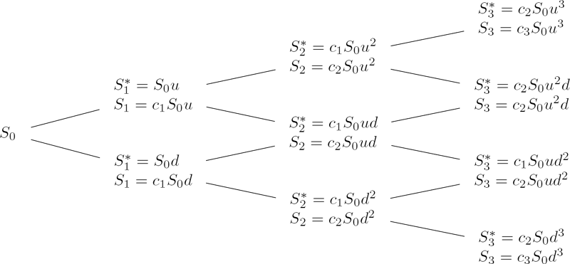
A three-period recombining tree for the asset price process with dividend payments Dt = qtSt*. Here ct = (1 − q1)(1 − q2) ··· (1 − qt) is the cumulative after-dividend factor.
asset price just prior to the dividend payment. The no-arbitrage asset price just after the dividend payment is
In the binomial model, the asset prices satisfy the following recurrence relation:
where the factor equals u with probability p or d with probability 1 − p, and it is independent of St−1. Applying the relation sequentially at times t, t − 1, ..., 1 gives
where ct is the cumulative after-dividend factor defined by
The evolution of the asset price process can be represented by a recombining binomial tree (see a three-period tree presented in Figure 7.14).
In the general case, where the dividend payments, {Dt}1≤t≤T, are not given as a percentage of the asset price, the recurrence formula for the asset price takes the form:
In general, the price dynamics of such an asset cannot be represented by a recombining binomial tree. In the case of rare dividend payments, we have a partly recombining tree.
Consider the three-period binomial tree model in Example 7.1 with S0 = 8, , , and . Assume the stock pays dividends at times t = 2 and t = 3 and each dividend payment is 10% of the stock price. That is, q1 = 0 and q2 = q3 = 0.1.
- (a) Construct the binomial tree with prior-and post-dividend stock prices.
- (b) Find and compare the prices of the standard European and American call options with common strike K = 6 and expiration T = 3.
Solution. The recombining binomial tree for the stock price process is given in Figure 7.1. The risk-neutral probabilities are and . At each node of the tree, we apply recurrence formulae (7.34) and (7.69) to evaluate the respective prices of the European and American call options. Let CtE and CtA, respectively, denote the time-t prices of the European and American put options for t = 0, 1, 2, 3. At the expiration date, the option value must equal the payoff function: C3E(S) = C3A(S) = (S − 6)+ for S ∊ {0.9, 2.7, 8.1, 24.3}. To determine the price for the times before expiration, use the following recurrences:
As a result, we obtain the option prices given in Figure 7.16. The values of the American put are boxed at those nodes of the tree where the intrinsic value is greater than or equal to the continuation value. Therefore, the American call option should be exercised at time t = 2 when the stock price is S2 = 16.2, or at time t = 3 when the price S3 exceeds the strike K = 6. Note that the initial price of the American call, C0A, is strictly larger than that of the European call, C0E.
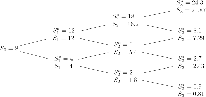
A three-period recombining binomial tree for the stock paying the dividend of 0.1 St* at times t = 1, 2.
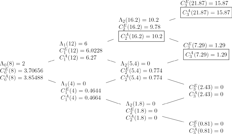
Prices of the standard European call, CtE, and American call, CtA, on the dividend-paying stock.
7.8 Exercises
- Exercise 7.1. Consider a T-period binomial tree model with stock price St, n = S0undt−n at each node (t, n) of the binomial tree for every n = 0, 1, ..., t and every t = 0, 1, ..., T.
- (a) Let v, t ∊ {0, 1, ..., T} be two dates such that v < t. Find the joint probability ℙ(St = St, n, Sv = Sv, m), n = 0, 1, ..., t, m = 0, 1, ..., v.
- (b) Find the conditional probability ℙ(St = St, n | Sv = Sv, m) using the result of (a).
- Exercise 7.2. Consider a three-period binomial model with S0 = 100, u = 1.15, and d = 0.9.
- (a) Find the distribution of S3 conditional on S1 = 115.
- (b) Find the distribution of S3 conditional on S1 = 90.
- Exercise 7.3. Consider a three-period binomial tree model with S0 = 8, u = 1.5, d = 0.5, and r = 0.25. Consider a European put option that expires at T = 3 and provides payoff (10 − S3)+. Let Pt, n be the price of this option at time t given that St = St, n.
- (a) Compute recursively backward in time the prices Pt, n, t = 3, 2, 1, 0, n = 0, 1, . . . , t. Present the prices calculated in a recombining binomial tree diagram.
- (b) Construct a hedging strategy {Δt}t = 0, 1, 2. Represent it using a recombining binomial tree diagram.
- Exercise 7.4. Complete the proof of Theorem 7.6 by showing that
- Exercise 7.5. Prove Theorem 7.7.
- Exercise 7.6. Find the initial risk-neutral value of a contract that pays $1 at the first time t when #U(ω1, ω2, ..., ωt) = n for some nonrandom n ∊ {1, 2, ..., T}.
Exercise 7.7. Consider a T-period binomial tree model. For t ≥ 0, define to be the geometric average of stock prices between times zero and t. Consider an Asian call option that expires at time T and provides payoff (GT − K)+ with strike price K. Let Vt(S, G) denote the price of this option at time t ≥ 0 given that St = S and Gt = G. In particular, VT (S, G) = (G − K)+.
- (a) Develop a one-step pricing formula for Vt = Vt(S, G) in terms of Vt+1, S, and G.
- (b) Develop a formula for Δt(S, G), the number of shares of stock held in a replicating portfolio during the period [t, t + 1], given that St = S and Gt = G.
- Exercise 7.8. Consider a three-period binomial model with S0 = 8, u = 1.5, d = 0.5, and r = 0.25. Consider an Asian call option that expires at time three and provides payoff (G3 − 8)+.
- (a) Compute the prices Vt for each t = 3, 2, 1, 0, using a backward-time recursion. Write these prices on a nonrecombining binomial tree diagram.
- (b) Construct a hedging strategy {Δt}t = 0, 1, 2. Represent it on a nonrecombining binomial tree diagram.
- Exercise 7.9. Consider a binomial-tree arbitrage-free model with T periods and arithmetic floating-price (Asian) call and put options with respective payoff functions
where K > 0 is a strike price and .
- (a) Find the risk-neutral conditional expectation .
- (b) Using the result of (a), find the put-call parity for the Asian options at time 0. That is, express the difference of initial prices C0 − P0 in terms of S0, K, T, and r.
- Exercise 7.10. Consider a T-period arbitrage-free binomial model and floating-price look-back call and put options with fixed strike K > 0 defined by the respective payoffs
where Mt : = max0≤n≤t Sn for 0 ≤ t ≤ T.
- (a) Prove (or argue) whether the floating-price lookback call and put option prices Ct and Pt at arbitrary time 0 ≤ t ≤ T are functions of the pair of values (Mt, St) or whether they are just functions of Mt.
- (b) Assume ud = 1 (i.e., a symmetric stock lattice) and T = 3 (i.e., a three-period model). Determine the arbitrage-free present values C0 and P0. Leave your answers as expressions in terms of the parameters S0, r, u, d.
Exercise 7.11. Consider the T-period binomial model with dividend-paying stock where the stock price process {St}0≤t≤T follows
with and . In this case the wealth equation takes the form
where r is a constant interest rate and Bt = (1 + r)t is the value at time t = 0, 1, ..., T of one dollar initially invested in the bank account at time 0.
- (a) Show that the discounted wealth process is a martingale under the risk-neutral measure . Hence, w.r.t. this measure, state the risk-neutral pricing formula for the price of a derivative claim at time n with payoff ΠT at terminal time T.
- (b) Show that the discounted stock price process is not a martingale but a strict supermartingale under the -measure, i.e., show that .
- (c) Denote ct = (1 − q1)(1 − q2) ··· (1 − qt). Clearly, ct is ℱt-measurable. Show that the process is a -martingale.
- Exercise 7.12. Consider the T-period binomial model with stock price St, n = S0undt−n each node (t, n) with t = 0, 1, ..., T and n = 0, 1, ..., t. Let Vt,n = Vt(St, n) denote the (no-arbitrage) price of any standard (non-path-dependent) European option at the node (t, n); let the relative derivative prices be defined by . Determine α and β (explicitly in terms of the model parameters) in the recurrence relation:
- Exercise 7.13. Consider a standard T-period binomial model and an Arrow–Debreu derivative security that pays one dollar if the single particular sequence of T market moves occurs and pays zero otherwise. Hence, this is a derivative with payoff given by the indicator function random variable :
- (a) Derive a formula for the no-arbitrage derivative value, Et, for time t = 0, 1, ..., T.
- (b) Consider the self-financed replicating portfolio strategy for this derivative. Derive a formula for the delta hedging position in the stock, Δt(ω1ω2 ··· ωt), for time t = 0, 1, ..., T − 1.
- Exercise 7.14. (The Law of One Price for the Binomial Tree Model). Consider two securities with respective discrete-time price processes {Xt}0≤t≤T and {Yt}0≤t≤T adapted to the binomial filtration . Suppose that XT(ω) = YT(ω) for all ω ∊ ΩT. Prove that Xt(ω1 ... ωt) = Yt(ω1 ... ωt) for all 0 ≤ t ≤ T and ω1, ..., ωt ∊ {D, U}, or else an arbitrage opportunity exists.
Exercise 7.15. Consider a T-period binomial arbitrage-free model and a chooser option expiring at time T with payoff
Derive the risk-neutral pricing formula in terms of the cumulative probability mass function of the binomial distribution Bin(n, p) given by
- Exercise 7.16. Consider a T-period binomial arbitrage-free model and a European-style derivative expiring at time T, namely,
(a) an asset-or-nothing call option with payoff
(b) a bear spread with payoff
(c) a strangle with payoff
Assume that K1 < S0 < K2 in (b) and (c). Derive the risk-neutral pricing formula in terms of the cumulative probability mass function of the binomial distribution.
- Exercise 7.17. Let σ > 0 and r∞ ≥ 0 be, respectively, an annual volatility and annual rate of interest compounded continuously. Consider the following parameterization of an N-period binomial model with the length of each period equal to :
Show that the binomial model is arbitrage free iff holds.
Exercise 7.18. Consider a 3-month call option on a dividend-paying stock with spot price S0 = $50 and strike price K = $51. The dividend is due at the end of month 1 and is equal to $2.50. Use a three-period binomial model with annual interest rate r∞ = 5% and annual volatility σ = 12% parametrized as in Exercise 7.17. Find the no-arbitrage initial values of
- (a) the European derivative,
- (b) the American derivative.
- Exercise 7.19. In the three-period binomial model with S0 = 8, u = 1.5, d = 0.5, and 1 + r = 1.25, determine the derivative prices, the delta hedging strategy, the consumption process, and the optimal stopping time for the American straddle that expiries at T = 3 and has intrinsic value Λ(S) = (8 − S)+ +(S − 8)+.
- Exercise 7.20. In the three-period binomial model with S0 = 8, u = 1.5, d = 0.5, and 1 + r = 1.25, determine the derivative prices, the delta hedging strategy, the consumption process, and the optimal stopping time for the American-Asian put that expiries at time three and whose intrinsic value at each time t = 0, 1, 2, 3 is
- Exercise 7.21. Consider the American derivative of Example 7.20. Find the optimal exercise policy (optimal stopping time) τ*. Verify that the initial derivative price is equal to