Chapter 14

American Options

In this chapter we briefly present the theory for pricing early-exercise (American) options in continuous time. Recall that American options were first introduced in Chapter 4, and the discrete-time case was dealt with in Chapter 7. Let us recall some of the properties of early-exercise options. The key difference between European-style and American-style options is that a holder of an American option can exercise her rights any time before the expiration date. This additional early exercise privilege should not be worthless. Thus, an American option is expected to be worth more than its European analogue. The extra premium paid on top of the price of the European option is called the early-exercise premium. We mainly focus our discussion on standard American call and put options with respective payoffs (S − K)+ and (K − S)+, although the theory can also be applied to other types of options. Throughout this chapter, we assume that we deal with only one underlying whose asset price process, {S(t)}t≽0, follows the standard geometric Brownian motion model, the risk-neutral dynamics of which is given by

$S\left(t\right)=S\left(0\right){\text{e}}^{\left(r-q-{\sigma }^2/2\right)t+\sigma \tilde{W}\left(t\right)},t\succcurlyeq 0.\text{ (14.1)}$

Here, r ≽ 0 is the risk-free interest rate, q ≽ 0 is the continuous dividend yield, σ > 0 is the asset price volatility, and ${\left\{\tilde{W}\left(t\right)\right\}}_{t\succcurlyeq 0}$ is a Brownian motion considered under the risk-neutral probability measure $\tilde{\mathbb{P}}$ with the bank account as the numéraire asset.

14.1 Basic Properties of Early-Exercise Options

Let t0 ≽ 0 be the contract inception time. American call and put options struck at K with expiration time T > t0 are claims to payoffs (S(t)−K)+ and (K −S(t))+, respectively, that the holder can exercise at any intermediate time t ∊ [t0, T]. As in previous chapters, the time-t value of an option with expiration date T is denoted by V (t, S), where S is the current asset (spot) price and t ∊ [t0, T] is the calendar time. It is also convenient to express the option value as a function of the time to expiration $\mathcal{T}$ = T − t when the asset price model is assumed to be a time-homogeneous stochastic process; the option value therefore depends on $\mathcal{T}$ and, as in previous chapters, we also denote the pricing function as v($\mathcal{T}$,S), where v(T − t, S) = V (t, S).

An American option cannot be worth less than its corresponding intrinsic value, which is the payoff associated with immediate exercise. In contrast to the case of European calls and puts, whose no-arbitrage values satisfy a put-call parity, there exists a put-call estimate for American options, which gives lower and upper bounds on the difference of call and put values (see Equation (4.8) and Exercise 4.8):

$S{\text{e}}^{-qT}-K\preccurlyeq C\left(T,S\right)-P\left(T,S\right)\preccurlyeq S-K{\text{e}}^{-rT},$

where C and P denote the prices of the American call and put options, respectively, with spot S and time to maturity τ . In the absence of dividends on the underlying asset, there is no advantage in exercising an American call prior to the expiry date. Hence, the American call being exercised at the expiration date is equivalent to its European counterpart (with the same strike and expiration). As a result, the American and European calls on a stock without dividends have the same value. If the stock pays dividends, the arguments above are not valid. The optimal exercise date depends on the dividend process. If dividends occur occasionally at certain dates, it may be optimal to exercise an American call option right before a dividend payment that is large enough. Therefore, in the presence of dividends, the American call can be worth more than the European call. Recall that this situation was studied for a binomial tree model in Chapter 7. Let us generalize our findings about relationships between American and European call/put options in the following propositions.

Proposition 14.1.

Let VE and V, respectively, denote the values of European and American options having the same payoff Λ(S) and expiration date T . The following two conditions are equivalent:

1. (i) VE (t, S) ≽ Λ (S) for all S > 0 and all t ∊ [t0, T];
2. (ii) V (t, S) = VE(t, S) for all S > 0 and all t ∊ [t0, T].

That is, if the corresponding European price is always above the intrinsic value during the contract lifetime, then it is never optimal to exercise the American option at any time earlier than expiry, i.e., there is no early-exercise premium and V ≡ VE.

Proof. For any time t, the value VE (t, S) is the arbitrage-free price of a contract exercised at the expiry time T. Condition (i) implies that it is not optimal to exercise earlier for a lower value. For every time t, it is more beneficial to wait until expiration. The optimal exercise (stopping) time is therefore at expiry T. Hence, (i) implies (ii). To prove the converse, observe that the American option value is always above the intrinsic value, i.e., V(t, S) ≽ (S) for all (t, S). Hence, condition (ii) implies (i). This result is essentially a statement of the fact that an early-exercise opportunity (and premium) arises if and only if the corresponding European option value falls below the intrinsic (payoff function) value.

As a corollary of Proposition 14.1, we have the rather well-known result:

Proposition 14.2.

1. (1) An American call has a nonzero early-exercise premium if and only if q > 0.
2. (2) An American put has a nonzero early-exercise premium if and only if r > 0.

This result follows from an arbitrage-free argument. However, a simple and instructive proof goes as follows.

Proof. Recall the put-call parity relation for European call and put options with common expiry T and strike price K:

$C^E\left(t,S\right)-P^E\left(t,S\right)={\text{e}}^{-q\left(T-t\right)}S-{\text{e}}^{-r\left(T-t\right)}K.$

Using the fact that PE(t, S) ≽ 0 gives

$C^E\left(t,S\right)=P^E\left(t,S\right)+{\text{e}}^{-q\left(T-t\right)}S-{\text{e}}^{-r\left(T-t\right)}K\succcurlyeq {\text{e}}^{-q\left(T-t\right)}S-K.\text{ (14.2)}$

Then, for q = 0, (14.2) gives CE(t, S) ≽ S − K. Hence the European call value is always above its payoff function. From Proposition 14.1, we conclude that the European call value, CE(t, S), is equal to the American call value, C(t, S), so that the early-exercise premium is zero. For the case q > 0, we use (14.2) and note that since the European put is a decreasing function of S, there exist large enough values of S such that PE(t, S) + e−q(T −t)S−e−r(T −t)K < 0, i.e., CE(t, S) < S−K for some S > K. From the previous result we therefore have C(t, S) > CE(t, S) and hence conclude that the early-exercise premium is nonzero for q > 0. This proves (i), while statement (ii) is proved in a similar fashion by reversing the roles of S and q with K and r, respectively, and is left as an exercise.

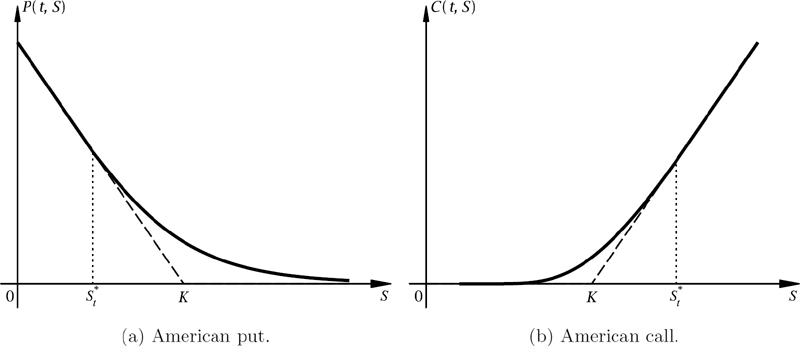
Statements (i) and (ii) are illustrated in Figures 14.1 and 14.2, respectively. If q > 0 (r > 0), then the graph of the call (put) option value function intersects the payoff diagram at some positive point Sc. For values of S greater (less) than Sc, the call (put) option price is strictly less than the payoff value. Note that P(t, 0) = e−r(T −t)K, which equals K if r = 0 and is less that K if r > 0, for all T − t > 0.

When we considered the no-arbitrage valuation of options under the binomial tree model, we analyzed the pricing of American options from both holder’s and writer’s points of view. The writer sells an option in exchange for some initial capital which can be used to hedge the short position in the derivative. This initial capital should provide the writer with sufficient funds to fulfil her obligations when the option is exercised. It is possible to find the best time for the holder (which is the worst time for the writer) to exercise the option. This time is called the optimal exercise time. The fair initial price of an American option is then defined as the smallest initial capital required to be hedged against exercise at the optimal time. Although the optimal exercise is not known in advance, the holder wishes to exercise the option as optimally as possible. Because the writer has no control over what exercise policy will be used by the buyer, the initial fair value of an American derivative with intrinsic value Λ(S) is defined as the maximum of ${\tilde{\text{E}}}_0\left[{\text{e}}^{-r\mathcal{T}}\Lambda \left(S\left(\mathcal{T}\right)\right)\right]$ over all possible exercise polices $\mathcal{T}\in \left[t_0,T\right]$. It can be shown that both approaches give the same value. In the next section, we carry out this analysis in continuous time.

14.2 Arbitrage-Free Pricing of American Options

14.2.1 Optimal Stopping Formulation and Early-Exercise Boundary

Consider an American option issued at time t0 ≽ 0 with payoff (intrinsic) value function Λ and expiration time T > t0. Suppose that the option has not been exercised before time t ∊ [t0, T]. Additionally, suppose that the holder of the option follows some exercise policy $\mathcal{T}$, which is a stopping time taking values in the interval [t, T] or taking the value ∞. Recall that St,T denotes the collection of all such stopping times. The no-arbitrage time-t value of the option, with underlying spot S, under a given exercise policy $\mathcal{T}$ is given by

${\tilde{\text{E}}}_{t,S}\left[{\text{e}}^{-r\left(\mathcal{T}-t\right)}\Lambda \left(S\left(\mathcal{T}\right)\right)\right].$

Note that we are using our previous shorthand notation for the conditional expectation ${\tilde{\text{E}}}_{t,S}[\cdot ]\equiv \tilde{\text{E}}\left[\cdot |S\left(t\right)=S\right]$. If $\mathcal{T}$ is infinite, we set e−r∞ Λ(S(∞)) to be zero. Under of what exercise rule will be used by the holder, the time-t value of an American option is defined to be

$V\left(t,S\right)=\underset{\mathcal{T}\in S_{t,T}}{\sup }{\tilde{\text{E}}}_{t,S}\left[{\text{e}}^{-r\left(\mathcal{T}-t\right)}\Lambda \left(S\left(\mathcal{T}\right)\right)\right].\text{ (14.3)}$

The optimal stopping time $\mathcal{T}$* maximizes the expectation on the right-hand side of (14.3). In other words, $\mathcal{T}$* is given implicitly by

$V\left(t,S\right)={\tilde{\text{E}}}_{t,S}\left[{\text{e}}^{-r\left({\mathcal{T}}^{*}-t\right)}\Lambda \left(S\left({\mathcal{T}}^{*}\right)\right)\right].\text{ (14.4)}$

By analogy with the case of the binomial tree model, the optimal exercise time $\mathcal{T}$* is the random variable corresponding to the first time when the option value equals the intrinsic value,

${\mathcal{T}}^{*}=\min \left\{u:t\preccurlyeq u\preccurlyeq T,V\left(u,S\left(u\right)\right)=\Lambda \left(S\left(u\right)\right)\right\}.\text{ (14.5)}$

That is, for maximal gain, along a stock price path (u, S(u, ω))t≼u≼T, the option should be exercised at the first time, say u = t* = $\mathcal{T}$*(ω), when V(t*, S(t*)) = Λ(S(t*)). Thus, letting S(t) = S, the (t, S)-plane consisting of the time and spot value points is separated into two sub-domains: a stopping domain where the option is exercised early,

$\mathcal{D}=\left\{\left(t,S\right):t_0\preccurlyeq t\preccurlyeq T,V\left(t,S\right)=\Lambda \left(S\right)\right\},\text{ (14.6)}$

and a continuation domain for which the option is not exercised,

${\mathcal{D}}^c=\left\{\left(t,S\right):t_0\preccurlyeq t\preccurlyeq T,V\left(t,S\right)>\Lambda \left(S\right)\right\},\text{ (14.7)}$

The continuation domain is the complement of the stopping domain within the rectangle [t0, T] × [0, ∞). As is seen from (14.6), the continuation domain is the set of all points (t, S) such that the option value V(t, S) exceeds the value of the payoff function Λ(S).

The geometry of the stopping domain may be quite complicated. It depends on the payoff function Λ and whether the underlying asset pays discrete dividends. However, for the case with a standard call/put payoff and continuous dividends, the stopping domain turns out to be simply connected. A typical shape of the stopping domain for a standard American put option is demonstrated in Figure 14.3. The early-exercise boundary, ∂D, which separates the continuation and stopping domains, is a smooth curve on the (t, S)-plane and is of the form $\partial \mathcal{D}=\left\{\left(t,S\right):0\preccurlyeq t\preccurlyeq T,S=S_t^{*}\right\}$, where the function S*t is given by

$S_t^{*}=\min \left\{S>0:V\left(t,S\right)={\left(S-K\right)}^{+}\right\}\text{ (14.8)}$

for a call and

$S_t^{*}=\max \left\{S>0:V\left(t,S\right)={\left(K-S\right)}^{+}\right\}\text{ (14.9)}$

for a put. Here, V represents the value of an American call, C, or put, P , respectively. Since the American option value is always nonnegative, the superscript + signs in (14.8) and (14.9) are actually redundant. Because the option value is positive, the critical value S*t is larger than the strike K for the American call and it is less than K for the American put.

In general, the early-exercise curve S*t varies with time t. For a given calendar time t ∊ [t0, T], we define the continuation and stopping intervals in [0, ∞) for spot price S, denoted by ${\mathcal{D}}_t^c$ and ${\mathcal{D}}_t$, respectively, so that $\mathcal{S}\in {\mathcal{D}}_t$ iff $\left(t,S\right)\in \mathcal{D}$ and ${\mathcal{D}}_t^c:=\left[0,\infty \right){\mathcal{D}}_t$. For a given time t, the American option is exercised if $\mathcal{S}\in {\mathcal{D}}_t$, and its value is equal to the payoff function in ${\mathcal{D}}_t$. For the American call, we have ${\mathcal{D}}_t^c=\left[0,S_t^{*}\right)$ and ${\mathcal{D}}_t=\left[S_t^{*},\infty \right)$; while for the American put, we have ${\mathcal{D}}_t^c=\left(S_t^{*},\infty \right)$ and ${\mathcal{D}}_t=\left[0,S_t^{*}\right]$. When S is in the stopping domain Dt, the values of the American call and put are C(t, S) = S − K and P(t, S) = K − S, respectively. In what follows, it will be convenient to express quantities in terms of time to maturity $\mathcal{T}$ = T − t. Consequently, we adopt the notations $S^{*}\left(T\right)\equiv S_t^{*},\mathcal{D}\left(T\right)\equiv {\mathcal{D}}_t$, and ${\mathcal{D}}^c\left(T\right)\equiv {\mathcal{D}}_t^c$.

An obvious consequence of Proposition 14.2 is that (a) for an American call on a non-dividend-paying stock the exercise boundary is trivial (i.e., it is never optimal to exercise early where ${\mathcal{D}}^c\left(\mathcal{T}\right)=\left[0,\infty \right)$) and (b) for an American put on a non-dividend-paying stock the exercise boundary is nontrivial (i.e., there is an optimal early-exercise time) if the interest rate is positive.

Note that for a general payoff function, the stopping domain may consist of several disconnected regions; therefore, the early-exercise boundary may be a union of separate curves. For example, in the case of an American strangle whose payoff is a sum of standard call and put payoffs, the stopping domain consists of upper and lower regions (assuming that both r and q are strictly positive).

As follows from the definition of the stopping domain, the optimal exercise time $\mathcal{T}$* defined in (14.5) is also the first passage time of the stopping domain $\mathcal{D}$. That is, the time $\mathcal{T}$* is the first time when the stock price process reaches the early-exercise boundary S* (see Figure 14.4):

${\mathcal{T}}^{*}=\min \left\{t\in \left[t_0,T\right]:S\left(t\right)=S_t^{*}\right\}.\text{ (14.10)}$

14.2.2 The Smooth Pasting Condition

The American option should be exercised whenever the asset price S is in the stopping domain $\mathcal{D}$. This implies that the American option value V(t, S) can be written as a piecewise continuous function of S which is equal to the payoff for all spot values $S\in {\mathcal{D}}_t$. For standard American call and put options, we have that C(t, S) = (S − K)+ = S − K if S ≽ S*t and P(t, S) = (K − S)+ = K − S if S ≼ S*t, respectively. Clearly, the option value functions have to be continuous at the exercise boundary point S = S*t or otherwise there exists an arbitrage opportunity. Moreover, as is demonstrated below, the optimal exercise condition requires the curve of V(t, S) to be tangent to the payoff at the point S*t. In other words, the pricing function for an American option has a continuous derivative at the exercise boundary; that is, the delta of the option price is continuous at the early-exercise boundary. This property is known as the smooth pasting condition.

We need to prove that the derivative of the option pricing function is equal to the derivative of the payoff function at the point S = S*t for any t ∊ [t0, T]. Let us first consider the case with a put option. Note that the argument presented below also readily follows for any continuous and monotonic payoff function such as the standard call and put payoffs. Suppose that the American put has not been exercised before time t. Consider the collection ℬ of all possible early-exercise boundaries defined by continuous functions b: [t, T] ω ℝ+. For each b ∊ ℬ, there is an exercise policy ${\mathcal{T}}_b$, which is the first passage time for the boundary b. Let

$P\left(t,S;b\right)={\tilde{\text{E}}}_{t,S}\left[{\text{e}}^{-r\left(T_b-t\right)}{\left(K-S\left(T_b\right)\right)}^{+}\right]$

be the put value under the exercise policy ${\mathcal{T}}_b$. Since every policy ${\mathcal{T}}_b$ is a stopping time in the set ${\mathcal{S}}_{\left[t,T\right]}$ and the function S*t of time t, defining the optimal exercise boundary, belongs to the collection ℬ, the value of the American put in (14.3) is given by P(t, S) = supb∊ℬ P(t, S; b). The optimal exercise boundary b = S* maximizes the function b ↦ P(t, S; b). So, this is a problem in calculus of variations. In general, if u is a function and F(u) is some functional of u, then the calculus of variations is a technique that tries to find such a u that optimizes F. If u* is an optimal solution, the functional derivative $\frac{\text{d}F\left(u\right)}{\text{d}u}$ is zero at u = u*. Since the optimal choice for the boundary b is the optimal early-exercise boundary S*, the derivative of the put value P with respect to b is zero at b = S*:

$\frac{\partial P\left(t,S;b\right)}{\partial b}{|}_{b=S^{*}}=0.$

Let us find the total derivative of the function P with respect to b along the boundary:

$\frac{\text{d}P}{\text{d}b}=\frac{\partial P\left(t,S;b\right)}{\partial S}{|}_{S=b}+\frac{\partial P\left(t,S;b\right)}{\partial b}{|}_{S=b},$

where we use the fact that $\frac{\partial S}{\partial b}=1$ along the curve S = b(t). On the one hand, when b = S*, we have $\frac{\text{d}P}{\text{d}b}=\frac{\partial P\left(t,S;b\right)}{\partial S}{|}_{S=S*}$. On the other hand, the option value is equal to the payoff function when S = b. Therefore, P(t, b; b) = (K − b) and then

$\frac{\text{d}P}{\text{d}b}\left(t,b;b\right)=\frac{\text{d}}{\text{d}b}\left(K-b\right)=-1.$

Putting the results together gives

$\frac{\partial P\left(t,S\right)}{\partial S}{|}_{S=S^{*}}=\frac{\partial P\left(t,S;S^{*}\right)}{\partial S}{|}_{S=S^{*}}=-1=\frac{\text{d}\Lambda \left(S\right)}{\text{d}S}{|}_{S=S^{*}}.\text{ (14.11)}$

where Λ(S) = (K − S)+ is the put payoff and equals K − S for all S < K. Note that S* < K for a put.

An alternative proof of the smooth pasting condition (14.11) is based on the no-arbitrage argument. If S < S*t, then P(t, S) = K − S. Therefore, the limit from the left is ${\lim }_{S\nearrow S_t^{*}}\frac{\partial P\left(t,S\right)}{\partial S}=-1$. Now consider the limit from the right. Since the American put value is always above the payoff values, we have ${\lim }_{S\searrow S_t^{*}}\frac{\partial P\left(t,S\right)}{\partial S}\succcurlyeq -1$. Our objective is to show that this inequality is actually a strict equality. We prove this by showing that there exists an arbitrage if the limiting value is strictly greater than −1. Suppose that the asset price at calendar time t is at the boundary, i.e., S ≡ S(t) = S*t. Consider a portfolio of one long put option and one share of stock. The portfolio value is

$\Pi \left(t\right)=S+P\left(t,S\right)=S+K-S=K.$

After a sufficiently small time lapse δt, the asset price can move downward into the exercise domain or upward into the continuation domain. We denote the change in the asset price by δS = S(t + δt) − S(t), so S(t + δt) = S + δS. If δS < 0, then P(t + δt, S + δS) = K −(S + δS) and the change in the portfolio value is δΠ = δP + δS = 0. If δS > 0, the small move δS creates a profit opportunity since δS > 0 and δP < 0 but in absolute value δP is smaller than δS. We thus have δΠ > 0. Let us find the order of magnitude of δΠ. Using the stochastic differential equation for the asset price process gives δS = μSδt + σSδW , where δW ~ Norm(0, δt). Therefore, we have

$\begin{array}{l}\delta \Pi =\delta S+\delta P=\delta S+\frac{\partial P}{\partial S}{|}_{S\searrow S_t^{*}}\delta S+\frac{1}{2}\frac{{\partial }^{2}P}{\partial S^2}{|}_{S\searrow S_t^{*}}{\left(\delta S\right)}^2+o\left(\delta t\right)\hfill \\ =\mathcal{O}\left(\delta t\right)+\left(\sigma S+\frac{\partial P}{\partial S}{|}_{S\searrow S_t^{*}}\sigma S\right)\delta W=\mathcal{O}\left(\delta t\right)+\left(1+\frac{\partial P}{\partial S}{|}_{S\searrow S_t^{*}}\right)\sigma S\sqrt{\delta t}|Z|,\hfill \end{array}$

where Z ~ Norm(0, 1), since δW > 0 for an upward movement of the stock price. Thus,

${\text{E}}_t\left[\delta \Pi |\delta S>0\right]=\mathcal{O}\left(\delta t\right)+\left(1+\frac{\partial P}{\partial S}{|}_{S\searrow S_t^{*}}\right)\sigma S\sqrt{\delta t}.$

This represents the change in portfolio value conditional on the stock price having a positive change within an arbitrarily small time interval δt. Since the term in $\sqrt{\delta t}$ is arbitrarily larger than all other terms of order $\mathcal{O}\left(\delta t\right)$, the change in portfolio value is positive if $\frac{\partial P}{\partial S}{|}_{S\searrow S_t^{*}}>-1$, i.e., the upward return on the portfolio is positive and of order $\sqrt{\delta t}$. This is an arbitrage opportunity since the risk-free return should be a smaller quantity. Therefore, the condition (14.11) holds. In fact, the smooth pasting condition is applicable to all types of American options. The general result is presented below without a proof.

Proposition 14.3.

Consider an American option with a differentiable payoff function Λ at any point (t, S*t) on the early-exercise boundary. Then, the American option pricing function V satisfies the smooth pasting condition:

$\frac{\partial V\left(t,S\right)}{\partial S}{|}_{S=S_t^{*}}={\Lambda }^{\prime }\left(S_t^{*}\right),\text{ (14.12)}$

that is, the (spacial) derivative of V is continuous at the boundary of the stopping and continuation domains (as is illustrated in Figure 14.5). Additionally, the option value V satisfies the zero time-decay condition on the early-exercise domain,

$\frac{\partial V\left(t,S\right)}{\partial t}=0,forallS\in {\mathcal{D}}_t.\text{ (14.13)}$

Proof. The proof is left as an exercise for the reader.

Remarks:

1. The condition in (14.12) is also obviously valid for all $\mathcal{S}\in {\mathcal{D}}_t$ since V(t, S) = Λ(S) on that region.

2. For a call (or put) the property (14.12) simply gives

   $\frac{\partial V\left(t,S\right)}{\partial S}{|}_{S=S_t^{*}}=1\left(\text{or}-1\right).$

   This is illustrated in Figure 14.5.

3. The properties (14.12) and (14.13) are also valid under a general diffusion model.

14.2.3 Put-Call Symmetry Relation

An American option can be considered as providing the right to exchange one asset for another, namely, one share of the underlying stock worth S dollars (asset one) and K dollars of cash (asset two). Such an exchange can take place any time before expiration. So, a call option gives the right to exchange cash for one unit of stock (i.e., exchange asset two for asset one) while a put option gives the right to exchange one unit of stock for cash (i.e., exchange asset one for asset two). Assets one and two have dividend yields q and r, respectively. Given this similarity we might expect call and put prices to be equal when we interchange the role of the underlying stock and cash. Let P($\mathcal{T}$, S; K, r, q) and C($\mathcal{T}$, S; K, r, q) respectively denote the price of the American put and call options with asset price S, strike price K, time to expiration $\mathcal{T}$ , dividend yield q, and risk-free interest rate r. After interchanging the role of the underlying asset and cash, the price of the modified American put is P($\mathcal{T}$, K; S, q, r). Since the modified put is equivalent to the American call, we have

$P\left(\mathcal{T},K;S,q,r\right)=C\left(\mathcal{T},S;K,r,q\right).\text{ (14.14)}$

This symmetry between the value function of an American call and put is called the put-call symmetry relation. The result is true for both European and American styles of options. It is also true for both perpetual and finite-expiration contracts. The symmetry relation (14.14) implies that the prices of at-the-money (i.e., S = K) American call and put options are equal if r = q. A rigorous proof of this relation is left as an exercise for the reader (see Exercises 14.2–14.3).

14.2.4 Dynamic Programming Approach for Bermudan Options

Bermudans are contracts that essentially lie in between European and American derivatives. Exercise of a Bermudan option can only occur at a fixed set of dates. Let

$T:=\left\{t_j:j=1,2,...,M\right\}$

be the set of allowable exercise dates, t0 ≼ t1 < t2 < · · · < tM = T. On the one hand, the value of a Bermudan option is defined as the maximum arbitrage-free price of the contract under all possible exercise policies. Every exercise policy is a stopping time taking its values in the set T or taking the value ∞. Let ST denote the collection of all stopping times taking values in T ∪ {∞}. Assuming that the option has not been exercised before time t, its arbitrage-free value at time t is

$V\left(t,S\right)=\underset{\mathcal{T}\in S_{T\cap \left[t,T\right]}}{\sup }\tilde{\text{E}}\left[{\text{e}}^{-r\left(\mathcal{T}-t\right)}\Lambda \left(S\left(\mathcal{T}\right)\right)|S\left(t\right)=S\right],\text{ (14.15)}$

where the underlying asset price process {S(t)}t≽0 is assumed to be Markovian. We expect (14.15) to be a good approximation to (14.3) for small durations δtj = tj − tj−1 between the many exercise dates. As max δtj → 0 (and hence M → ∞), the Bermudan option value in (14.15) converges to the (continuous-time exercise) American option value (14.3).

Since the continuous-time process {S(t)}t≽0 is Markovian, S(t1), S(t2), . . . , S(tM) form a Markov chain. It can be shown that the Bermudan option values at the discrete exercise dates satisfy the recurrence relation

$\begin{array}{cc}\hfill V\left(t_j,S\right)=& \max \left\{\Lambda \left(S\right),{\tilde{\text{E}}}_{t_j}\left[{\text{e}}^{-r\left(t_{j+1}-t_j\right)}V\left(t_{j+1},S\left(t_{j+1}\right)\right)|S\left(t_j\right)=S\right]\right\}\hfill \\ \hfill :=& \max \left\{\Lambda \left(S\right),V^{cont}\left(t_j,S\right)\right\}\text{for}j=M-1,M-2,...,1,\hfill \end{array}\text{ (14.16)}$

where V(T, S) = Λ(S) at the expiration time T. The conditional expectation in (14.16) denoted by Vcont(t, S) represents the continuation value of the option at time ti. It is the time-t value of the option that has not been exercised yet at time t.

Let the asset price process be a continuous-time stochastic process with assumed risk-neutral transition PDF $\tilde{p}\left(t,t^{\prime };S,S^{\prime }\right):=\frac{\tilde{\mathbb{P}}\left(S\left(t^{\prime }\right)\in d{S}^{\prime }|S\left(t\right)=S\right)}{\text{d}{S}^{\prime }}$ with S, S′ > 0 and 0 ≼ t < t′. Then, the continuation value in (14.16) is computed as

$V^{cont}\left(t_j,S\right)={\text{e}}^{-r\left(t_{j+1}-t_j\right)}{\displaystyle {\int }_0^{\infty }\tilde{p}\left(t_j,t_{j+1};S,S^{\prime }\right)V\left(t_{j+1},S^{\prime }\right)}\text{d}{S}^{\prime }.$

Recall that in the case of a time-homogeneous process, the transition PDF only depends on the duration t′ − t rather than on the individual time moments t and t′, that is,

$\tilde{p}\left(t,t^{\prime };S,S^{\prime }\right)=\tilde{p}\left(t^{\prime }-t;S,S^{\prime }\right).$

In particular, recall that for the geometric Brownian motion model in (14.1), $\tilde{p}$ is the log-normal density given by (12.16) with r replaced by r − q.

The dynamic-programming formulation (14.16) of the Bermudan option pricing problem does not require computation of the early-exercise boundary. However, the optimal exercise rule and early-exercise boundary can be obtained simultaneously while computing option values. In particular, the optimal exercise rule is

${\mathcal{T}}^{*}=\text{min}\left\{t_j,j=1,2,...,M:\Lambda \left(S\left(t_j\right)\right)=V\left(t_j,S\left(t_j\right)\right)\right\}.$

Essentially, the rule is defined in the same way as that for the binomial tree model in Chapter 6. Since the Bermudan option can only be exercised at times from the set T, the stopping domain $\mathcal{D}\subset \left[0,T\right]\times {ℝ}_{+}$ is the union of lines

$\mathcal{D}={\displaystyle \underset{1\preccurlyeq j\preccurlyeq M}{\cup }\left\{\left(t_j,S\right):\Lambda \left(S\right)\succcurlyeq V^{cont}\left(t,S\right)\right\}.}$

The dynamic programming formulation of the American option pricing problem provides a basis for implementing a number of numerical methods for computing option prices using Monte Carlo simulations, finite-difference schemes, lattice methods, or a combination of such approaches. For a detailed exposition on the numerical methods for pricing American options, we refer the reader to the last chapter of this book.

14.3 Perpetual American Options

In this section, we consider a perpetual option with infinite time to expiration. That is, a perpetual option has no expiration date and can be exercised at any future time. Such options are not among traded securities. However, they are an instructive mathematical concept because they admit simple analytic solutions. In this section we derive closed-form pricing formulae for perpetual American calls and puts. Additionally, perpetual options represent an accurate approximation of finite-expiration American options when the time horizon of the expiry is very long.

Consider a perpetual derivative with intrinsic value δ(S). We are interested in its value as a function of the underlying asset price. The holder of a perpetual American option can exercise it at any time. Since the time to expiry is always infinite, the option value must be independent of time. That is, the value of a perpetual derivative, V , depends only on the asset price, i.e., we simply write V(t, S) = V(S) for all t ≽ 0. It is reasonable to expect that the early-exercise boundary that separates the continuation and stopping domains does not depend on the time variable t as well. The function S*t that describes the early-exercise boundary is constant, i.e., there is a fixed exercise level S*t = S* for all t ≽ 0. The stopping domain (on the time and stock price plane) is $\mathcal{D}={ℝ}_{+}\times \left(0,S^{*}\right]$ for a perpetual put option and $\mathcal{D}={ℝ}_{+}\times \left[S^{*},\infty \right)$ for a perpetual call option.

14.3.1 Pricing a Perpetual Put Option

Let us consider the case of a perpetual American put option with intrinsic value (K−S)+. The holder will exercise the option when it is deep enough in the money. That is, there exists some constant level S* ≼ K so that it is optimal to exercise as soon as the price S(t) reaches the level S*. From the definition of the optimal stopping time $\mathcal{T}$* as given in (14.4) and (14.10), we conclude that the value of a perpetual put, P(S) ≡ P(S; K, r, q), is

$P\left(S\right)={\tilde{\text{E}}}_{0,S}\left[{\text{e}}^{-r{\mathcal{T}}^{*}}\left(K-S\left({\mathcal{T}}^{*}\right)\right)\right]\text{ (14.17)}$

$=\left(K-S^{*}\right){\tilde{\text{E}}}_S\left[{\text{e}}^{-r{T}^{*}}\right]\text{for}S>S^{*}\text{ (14.18)}$

where ${\tilde{\text{E}}}_{0,S}\equiv {\tilde{\text{E}}}_S$ is the risk-neutral expectation conditional on S(0) = S, and $\mathcal{T}$* is the first passage time to the level S*, i.e.,

${\mathcal{T}}^{*}=\text{inf}\left\{t\succcurlyeq 0:S\left(t\right)=S^{*}\right\}.$

Under the assumption that the asset price follows the geometric Brownian motion model, the time $\mathcal{T}$* is the first passage time of the drifted Brownian motion $X\left(t\right)=\mu t+\tilde{W}\left(t\right)$, with drift $\mu =\frac{r-q-{\sigma }^2/2}{\sigma }$, to the level $L*=\frac{1}{\sigma }\ln \frac{S*}{S}$, i.e.,

${\mathcal{T}}^{*}=\text{inf}\left\{t\succcurlyeq 0:X\left(t\right)\preccurlyeq L^{*}\right\}.$

We recall from Section 10.4.2 of Chapter 10 that this corresponds to the first hitting time, ${\mathcal{T}}_{L*}^X$, of the drifted Brownian motion down to the level L* < 0 in case S > S*. The mathematical expectation in (14.18) is actually the Laplace transform of the PDF of $\mathcal{T}$*, evaluated at r. This Laplace transform can be readily obtained analytically. However, it can also be computed via the Feynman–Kac formula for processes stopped at a first passage time. In this case the stopping time $\mathcal{T}$* is the first hitting time to the level S*. In particular, the function $v\left(S\right)={\tilde{\text{E}}}_S\left[{\text{e}}^{-r\mathcal{T}*}\right]$ satisfies the ordinary differential equation (ODE) $\mathcal{G}\upsilon -r\upsilon =0$ where $\mathcal{G}$ is the Generator for the stock price process under the risk-neutral measure, i.e.,

$\frac{1}{2}{\sigma }^2{S}^2\frac{{\text{d}}^{2}v}{\text{d}{S}^2}+\left(r-q\right)S\frac{\text{d}v}{\text{d}S}-rv=0,S>S^{*},\text{ (14.19)}$

subject to the boundary conditions

$\left(\text{i}\right)v\left(S^{*}\right)=1,\left(\text{ii}\right)\underset{S\to \infty }{\lim }v\left(S\right)=0,\text{ (14.20)}$

where S* is yet unknown but uniquely determined once v(S) is obtained in terms of S*, as described just below. The first boundary condition corresponds to $\mathcal{T}$* being zero $\left({\text{e}}^{-r\mathcal{T}*}=1\right)$ if the process starts at S = S*. The second condition arises since $\mathcal{T}$* goes to infinity $\left({\text{e}}^{-r\mathcal{T}*}\to 0\right)$ as the process is started at an arbitrarily large value S (i.e., the point at infinity is a natural boundary for the stock price process).

The value of the perpetual put given by P(S) = (K − S*)v(S) satisfies the ODE (14.19) subject to

$\left(\text{i}\right)P\left(S^{*}\right)=\left(K-S^{*}\right),\left(\text{ii}\right)\underset{S\to \infty }{\lim }P\left(S\right)=0.\text{ (14.21)}$

Note that the ODE (14.19) is also obtained from the Black–Scholes partial differential equation (PDE) by setting the time derivative to zero. As is demonstrated below, the pricing function of a finite-expiration American option does indeed satisfy the Black–Scholes PDE (14.31) in the stopping domain. Since the perpetual option value V is time independent, the time derivative $\frac{\partial V}{\partial t}$ is identically zero. Hence, the Black–Scholes PDE (14.31) reduces to the ODE (14.19).

Equation (14.19) is of the Cauchy–Euler type, ax2y″(x) + bxy′(x) + cy(x) = 0, with constants a, b, and c. The general solution has the form $y\left(x\right)=A_1{x}^{{\lambda }_1}+A_2{x}^{{\lambda }_2}$, where A1 and A2 are arbitrary constants. Putting the function v(S) = S* into (14.19) gives the following auxiliary equation on the exponent λ:

$\frac{{\sigma }^2}{2}\lambda \left(\lambda -1\right)+\left(r-q\right)\lambda -r=0.$

Solving it gives

$\lambda ={\lambda }_{\pm }:=\frac{-\left(r-q-{\sigma }^2/2\right)\pm \sqrt{{\left(r-q-{\sigma }^2/2\right)}^2+2{\sigma }^{2}r}}{{\sigma }^2}.\text{ (14.22)}$

Assuming positive interest rate r, it is easy to show that λ− < 0 and λ+ > 0. So the general solution to (14.19) is $v\left(S\right)=a_{+}{S}^{{\lambda }_{+}}+a_{-}{S}^{{\lambda }_{-}}$. Now, we determine the coefficients a± in terms of S*. To satisfy condition (14.20(ii)),

$\underset{S\to \infty }{\lim }\left(a_{+}{S}^{\lambda +}+a_{-}{S}^{\lambda -}\right)=0,$

we must have a+ = 0. Then, a− is determined from condition (14.20(i)):

$v\left(S^{*}\right)=a_{-}{\left(S^{*}\right)}^{{\lambda }_{-}}=1$

for an arbitrary yet undetermined parameter S*. Thus, the solution to the problem (14.19)–(14.20) is

$v\left(S\right)={\left(\frac{S}{S^{*}}\right)}^{{\lambda }_{-}},S>S^{*}.$

In fact, the function v(S) is the price of a so-called digital option that pays $1 when the asset price breaches a lower level S*. The perpetual put value is then

$P\left(S\right)\equiv P\left(S;S^{*}\right)=\{\begin{array}{l}\left(K-S^{*}\right){\left(\frac{S}{S^{*}}\right)}^{{\lambda }_{-}},S^{*}<S,\hfill \\ K-S,0<S\preccurlyeq S^{*}.\hfill \end{array}\text{ (14.23)}$

The last step is to determine S*. Consider two methods: first, using the fact that S* must be the optimal value that maximizes the option value P(S) among all possible choices of S* > 0; second, using the smooth pasting condition. Let us find the maximum of the function S* ↦ P(S; S*). Differentiating the option value with respect to S* for S* < S gives

$\frac{\partial P}{\partial S^{*}}=\frac{\partial }{\partial S^{*}}\left\{\left(K-S^{*}\right){\left(\frac{S}{S^{*}}\right)}^{{\lambda }_{-}}\right\}=-{\left(\frac{S}{S^{*}}\right)}^{{\lambda }_{-}}\left(1+\frac{K-S^{*}}{S^{*}}{\lambda }_{-}\right).$

Set $\frac{\partial P}{\partial S*}=0$ to obtain the extremum

$S^{*}=\frac{K{\lambda }_{-}}{{\lambda }_{-}-1}.\text{ (14.24)}$

Note that $\frac{{\partial }^{2}P}{\partial {\left(S*\right)}^2}=\frac{K{\lambda }_{-}}{{\left(S*\right)}^2}{\left(\frac{S}{S*}\right)}^{{\lambda }_{-}}<0$ since λ− < 0. Thus, S* given by (14.24) is indeed a maximum. Finally, substituting (14.24) in (14.23) gives the perpetual put price:

$P\left(S;K,r,q\right)=\{\begin{array}{l}\frac{K}{1-{\lambda }_{-}}{\left(\frac{{\lambda }_{-}-1}{{\lambda }_{-}}\right)}^{\lambda -}{\left(\frac{S}{K}\right)}^{{\lambda }_{-}}=-\frac{S^{*}}{{\lambda }_{-}}{\left(\frac{S}{S^{*}}\right)}^{{\lambda }_{-}},S^{*}<S,\hfill \\ K-S,0<S\preccurlyeq S^{*}.\hfill \end{array}\text{ (14.25)}$

The solution in (14.25) is also readily obtained by applying the smooth pasting condition to the function in (14.23). Namely, we differentiate the function for S > S* and set the derivative to −1 at S = S*:

$\frac{\partial P}{\partial S}{|}_{S=S^{*}}=-{\lambda }_{-}\left(\frac{K-S^{*}}{S^{*}}\right)=-1.$

Solving the above equation for S* gives the optimal value in (14.24).

Let us examine what happens to the exercise boundary in the limiting case when the interest rate r is zero. From (14.22), we obtain λ− = 0. Thus, from (14.24) we see that S* = 0. Hence, for a zero interest rate, the perpetual put is never exercised early. This observation is consistent with the property of any finite-expiration American put.

14.3.2 Pricing a Perpetual Call Option

Now we consider the perpetual American call struck at K. Let C(S) ≡ C(S; K, r, q) denote its price when the stock price is equal to S. As in the case of the perpetual put option, the call pricing function C(S) satisfies the ODE (14.19) but now for S ∊ (0, S*). In the stopping domain [S*, ∞), the call value is equal to the payoff value, i.e.,

$C\left(S\right)=S-K\text{for}S\succcurlyeq S^{*}.$

Hence, the boundary conditions are

$\left(\text{i}\right)\underset{S\to 0+}{\lim }C\left(S\right)=0,\left(\text{ii}\right)C\left(S^{*}\right)=\left(S^{*}-K\right).\text{ (14.26)}$

The first condition states that the call is worthless if the stock price is zero since it will remain at zero indefinitely, i.e., the payoff is always zero. The general solution to (14.19) is $C\left(S\right)=a_{+}{S}^{{\lambda }_{+}}+a_{-}{S}^{{\lambda }_{-}}$, where the exponents λ± are given by (14.22). Since C(0+) = 0 and λ− < 0, we must set a− = 0. Imposing the condition (14.26(ii)) gives a+ = (S*−K)/(S*)*+. Following the same procedure as above, we obtain the optimal value of S*:

$S^{*}=\frac{K{\lambda }_{+}}{{\lambda }_{+}-1}.\text{ (14.27)}$

The perpetual call price is then

$C\left(S;K,r,q\right)=\{\begin{array}{l}\frac{K}{{\lambda }_{+}-1}{\left(\frac{{\lambda }_{+}-1}{{\lambda }_{+}}\right)}^{{\lambda }_{+}}{\left(\frac{S}{K}\right)}^{{\lambda }_{+}}=\frac{S^{*}}{{\lambda }_{+}}{\left(\frac{S}{S^{*}}\right)}^{{\lambda }_{+}},0<S<S^{*},\hfill \\ S-K,S^{*}\preccurlyeq S.\hfill \end{array}\text{ (14.28)}$

A simple check by differentiation shows that this function satisfies the required smooth pasting condition for a call,

$\frac{\partial C}{\partial S}{|}_{S=S^{*}}=1.$

Let us examine what happens to the exercise boundary in the limiting case when the dividend yield q is zero. From (14.22) and (14.27), we see that λ+ → 1 and S* → ∞ as q → 0+. Hence, for a zero dividend yield, the perpetual call is never exercised early. Again, this is consistent with the property of any finite-expiration American call.

14.4 Finite-Expiration American Options

14.4.1 The PDE Formulation

Pricing an American option can be formulated as a boundary initial value problem for a partial differential equation with a time-dependent free boundary. The solution domain is divisible into a union of a stopping region, $\mathcal{D}$, where the American option is exercised, and a continuation domain, ${\mathcal{D}}^c$, where the option is not exercised. Inside the continuation domain, the option value function satisfies the Black–Scholes PDE. On the early-exercise boundary, the option value is equal to the payoff function Λ(S). The early-exercise boundary is an unknown function of time which must also be determined as part of the solution. Here we assume the payoff is time independent, although the formulation also extends to the case of a time-dependent payoff.

Delta hedging and continuous-time replication arguments apply to American options in the same way as they apply to European options. Therefore, within the continuation domain the option pricing function must satisfy the Black–Scholes PDE. The connection between the optimal stopping time formulation and the PDE approach can be shown using the following heuristic. Consider the recurrence relation (14.16) for a calendar time t ∊ [t0, T] and a small time step δt > 0 :

$V\left(t,S\right)=\max \left\{\Lambda \left(S\right),{\text{e}}^{-r\delta t}\tilde{\text{E}}\left[V\left(t+\delta t,S\left(t+\delta t\right)\right)|S\left(t\right)=S\right]\right\}.$

Assuming V(t, S) is a sufficiently smooth function with continuous derivatives, we can expand V(t + δt, S(t + δt)) in a Taylor series while keeping terms up to $\mathcal{O}\left(\delta t\right)$. Assuming the underlying asset follows the GBM model in (14.1), we have:

$\begin{array}{cc}\hfill V\left(t,S\right)=& \max \{\Lambda \left(S\right),\left(1-r\delta t\right){\tilde{\text{E}}}_{t,S}[V\left(t,S\left(t\right)\right)+(\frac{\partial V\left(t,S\left(t\right)\right)}{\partial t}+\left(1-q\right)S\left(t\right)\frac{\partial V\left(t,S\left(t\right)\right)}{\partial S}\hfill \\ \hfill & +\frac{1}{2}{\sigma }^2{S}^2\left(t\right)\frac{{\partial }^{2}V\left(t,S\left(t\right)\right)}{\partial S^2})\delta t+\sigma S\left(t\right)\frac{\partial V\left(t,S\left(t\right)\right)}{\partial S}\delta {\tilde{W}}_t]\}+\mathcal{O}\left(\delta t^2\right)\hfill \\ \hfill =& \max \left\{\Lambda \left(S\right),V\left(t,S\right)+\left[\frac{\partial V\left(t,S\right)}{\partial t}+ℒV\left(t,S\right)\right]\delta t\right\}+\mathcal{O}\left(\delta t^2\right).\hfill \end{array}\text{ (14.29)}$

The second equation is obtained by evaluating the expectation conditional on S(t) = S and then collecting terms up to $\mathcal{O}\left(\delta t\right)$. Note that the coefficient terms multiplying δt and $\delta {\tilde{W}}_t$ are both ℱt-measurable with given spot value S(t) = S. Moreover, the conditional expectation term in $\delta {\tilde{W}}_t$ vanishes by the independence of the Brownian increment $\delta {\tilde{W}}_t={\tilde{W}}_{t+\delta t}-{\tilde{W}}_t$ and S(t), i.e., ${\tilde{\text{E}}}_{t,s}\left[S\left(t\right)\frac{\partial V\left(t,S\left(t\right)\right)}{\partial S}\delta {\tilde{W}}_t\right]=S\frac{\partial V\left(t,S\right)}{\partial S}{\tilde{\text{E}}}_{t,s}\left[\delta {\tilde{W}}_t\right]=0$ since ${\tilde{\text{E}}}_{t,s}\left[\delta {\tilde{W}}_t\right]=\tilde{\text{E}}\left[\delta {\tilde{W}}_t\right]=0$. The expression in (14.29) has been written more compactly using the Black–Scholes differential operator ℒ := $\mathcal{G}$ − r,

$ℒf:=\frac{1}{2}{\sigma }^2{S}^2\frac{{\partial }^{2}f}{\partial S^2}+\left(r-q\right)S\frac{\partial f}{\partial S}-rf.\text{ (14.30)}$

For values of S in the continuation domain ${\mathcal{D}}_t^c$ the inequality V(t, S) > Λ(S) is satisfied. In (14.29), we require the right-hand side to equal the left to small order o(δt). Hence, the coefficient in δt must be zero, which is the Black–Scholes PDE:

$\frac{\partial V\left(t,S\right)}{\partial t}+ℒV\left(t,S\right)=0,\text{for}\text{all}S\in {\mathcal{D}}_t^c\text{and}\text{all}t\in \left[t_0,T\right].$

Thanks to the time-homogeneous property of the solution, V(t, S) = v($\mathcal{T}$, S), we have a PDE in terms of the time to maturity variable $\mathcal{T}$ = T − t and spot S:

$\frac{\partial v\left(T,S\right)}{\partial T}+ℒv\left(t,S\right),\text{for}\text{all}S\in {\mathcal{D}}^c\left(T\right)\text{and}\text{all}T>0.\text{ (14.31)}$

The Black–Scholes PDE does not hold on the stopping domain, where the American option is given by the payoff function V(S, $\mathcal{T}$) = Λ(S). Since the payoff is time-independent, the derivative $\frac{\partial \Lambda \left(S\right)}{\partial T}$ is zero. Thus, the solution v($\mathcal{T}$, S) on $\mathcal{D}\left(\mathcal{T}\right)$ satisfies $\frac{\partial v}{\partial T}=0$. Combining regions and assuming the payoff is a twice differentiable function gives a nonhomogeneous Black–Scholes PDE valid in the whole region:

$\frac{\partial v\left(T,S\right)}{\partial T}=ℒv\left(T,S\right)+f\left(T,S\right),\text{ (14.32)}$

with function

$f\left(T,S\right)=\{\begin{array}{l}0,S\in {\mathcal{D}}^c\left(T\right),\hfill \\ -ℒ\Lambda \left(S\right),S\in \mathcal{D}\left(T\right).\hfill \end{array}\text{ (14.33)}$

Given the function f($\mathcal{T}$, S) whose time dependence is determined in terms of the early-exercise boundary, the solution to (14.32), subject to the initial condition

$v\left(0,S\right)=\Lambda \left(S\right)\text{ (14.34)}$

and the boundary conditions

$\underset{S\to 0+}{\lim }v\left(T,S\right)=\underset{S\to 0+}{\lim }\Lambda \left(S\right),\underset{S\to \infty }{\lim }v\left(T,S\right)=\underset{S\to \infty }{\lim }\Lambda \left(S\right),\text{ (14.35)}$

can be obtained in terms of the solution to the corresponding (homogeneous) Black–Scholes PDE, $\frac{\partial v\left(T,S\right)}{\partial T}=ℒv\left(T,S\right)$.

For the American call and put, we recall the early-exercise curves S = S*($\mathcal{T}$) expressed as a function of time to maturity on the (S, $\mathcal{T}$)-plane. For the call, the set of spot values $S\in \mathcal{D}\left(\mathcal{T}\right)$ is then equivalent to the set of values S ≽ S*(τ). For the put, the values $S\in \mathcal{D}\left(T\right)$ are the values S ≼ S*($\mathcal{T}$). Hence, expressing the call and put option values as functions of τ and S, (14.32) and (14.33) specialize to

$\frac{\partial C}{\partial T}-\frac{{\sigma }^2{S}^2}{2}\frac{{\partial }^{2}C}{\partial S^2}-\left(r-q\right)S\frac{\partial C}{\partial S}+rC=\{\begin{array}{l}0S<S^{*}\left(T\right),\hfill \\ qS-rK,S\succcurlyeq S^{*}\left(T\right),\hfill \end{array}\text{ (14.36)}$

and

$\frac{\partial P}{\partial T}-\frac{{\sigma }^2{S}^2}{2}\frac{{\partial }^{2}P}{\partial S^2}-\left(r-q\right)S\frac{\partial P}{\partial S}+rP=\{\begin{array}{l}rK-qSS\preccurlyeq S^{*}\left(T\right),\hfill \\ 0S>S^{*}\left(T\right),\hfill \end{array}\text{ (14.37)}$

respectively. For the call, we used the fact that −ℒΛ(S) = −ℒ(S − K) = −(rK − qS) = qS − rK. For the put, −ℒΛ(S) = −ℒ(K − S) = rK − qS. Here, we used S*($\mathcal{T}$) to denote the early-exercise boundary for the respective call and put with given strike K. The right-hand sides of these nonhomogeneous PDEs are nonzero only within the respective stopping regions.

We close this section by working out some other basic properties of the early-exercise boundary for a call and a put option. Let’s consider the limit of infinitesimally small $T\searrow 0$. In particular, consider an American call struck at K with continuous dividend yield q. The pricing function C($\mathcal{T}$, S; K), is an increasing function of τ, i.e., C(τ2, S; K) ≽ C($\mathcal{T}$1, S; K) for $\mathcal{T}$2 > $\mathcal{T}$1. Also, the smooth pasting condition guarantees that the pricing functions join the intrinsic line at levels S*($\mathcal{T}$1) − K and S*($\mathcal{T}$2) − K, respectively, giving S*($\mathcal{T}$2) > S*($\mathcal{T}$1). We hence conclude that S*($\mathcal{T}$) is a continuously increasing function of $\mathcal{T}$ > 0 and attains the value of the early-exercise boundary of the corresponding perpetual call option, given by (14.27), in the limit $\mathcal{T}$ → ∞. That is, an American call with greater time to maturity should be exercised deeper in the money to account for the loss of time value on the strike K. Since one would never prematurely exercise at a spot value that is below the strike level, the early-exercise boundary for an American call must satisfy the property S*($\mathcal{T}$) > K for all $\mathcal{T}$ > 0. To determine the boundary in the limit $T\searrow 0$, we note that the option value approaches the intrinsic value, i.e., at expiry the option value is given by the payoff C(S, K, $\mathcal{T}$ = 0) = S − K for values on the exercise boundary. According to (14.36) we have

$\frac{\partial C\left(S,K,0+\right)}{\partial T}=rK-qS\text{ (14.38)}$

for S > K. Since the condition ∂C(S, K, 0+)/∂$\mathcal{T}$ > 0 ensures that the option is not yet exercised, the spot value S at which ∂C(S, K, 0+)/∂$\mathcal{T}$ becomes negative and hence for which the call is exercised at an instant just before expiry is given by $S=\frac{r}{q}K$. This is the case, however, if the value $\frac{r}{q}K$ is in the interval S > K; that is if r > q > 0. In this case just prior to expiry the call is not yet exercised if the spot is in the region $K<S<\frac{r}{q}K$, but would be exercised if $S\succcurlyeq \frac{r}{q}K$. Hence, in the limiting case we have $S*\left(0+\right)=\frac{r}{q}K\text{for}r>q>0$. For the other case we have r ≼ q, so $\frac{r}{q}K\preccurlyeq K$. Yet S > K, so that S*(0+) = K for r > q. Note that the condition S*(0+) > K is not possible in this case as this leads to a sub-optimal early exercise since the loss in dividends would have greater value than the interest earned over the infinitesimal time interval until expiry. Combining the above arguments we arrive at the general limiting condition for the exercise boundary of an American call just prior to expiry:

$\underset{\mathcal{T}\searrow 0}{\lim }{S}^{*}\left(\mathcal{T}\right)=\max \left(K,\frac{r}{q}K\right)=K\max \left(1,\frac{r}{q}\right).\text{ (14.39)}$

From this property we see that S*(0+) → ∞ as q → 0. So, for zero dividend yield the American call is never exercised early which is consistent with the fact that the American call has exactly the same worth as the European call. By using similar arguments as above we readily work out S*(0+) for the Amercian put struck at K with continuous dividend yield q. For the put, S*($\mathcal{T}$) is a continuously decreasing function of $\mathcal{T}$ > 0 and attains the value in (14.24) in the limit $\mathcal{T}$ → ∞. We leave it as an exercise for the reader to show that

$\underset{T\searrow 0}{\lim }{S}^{*}\left(T\right)=K\min \left(1,\frac{r}{q}\right).\text{ (14.40)}$

14.4.2 The Integral Equation Formulation

Recall that the time-homogeneous risk-neutral transition PDF, $\tilde{p}=\tilde{p}\left(T;S,S^{\prime }\right)$, solves the forward Kolmogorov PDE in the S′ variable and the backward Kolmogorov PDE in the spot variable S with zero boundary conditions at S = 0 and S = ∞ for all $\mathcal{T}$ > 0. As mentioned above, for the process (14.1) the PDF $\tilde{p}$ is just the log-normal density. We also know that the function ${\text{e}}^{-r\mathcal{T}}\tilde{p}$ solves the (homogeneous) Black–Scholes PDE. Combining these facts and applying Laplace transforms, one arrives at the well-known Duhamel solution to (14.32) in the form

$\begin{array}{ll}\hfill v\left(\mathcal{T},S\right)=& {\text{e}}^{-r\mathcal{T}}{\displaystyle {\int }_0^{\infty }\tilde{p}\left(\mathcal{T};S,S^{\prime }\right)\Lambda \left(S^{\prime }\right)}\text{d}{S}^{\prime }+{\displaystyle {\int }_0^{\mathcal{T}}{\text{e}}^{-r{\mathcal{T}}^{\prime }}}\left[{\displaystyle {\int }_0^{\infty }\tilde{p}\left({\mathcal{T}}^{\prime };S,S^{\prime }\right)f\left(\mathcal{T}-{\mathcal{T}}^{\prime },S^{\prime }\right)\text{d}{S}^{\prime }}\right]\text{d}{\mathcal{T}}^{\prime }\hfill \\ \hfill \equiv & v^E\left(\mathcal{T},S\right)+v^e\left(\mathcal{T},S\right)\hfill \end{array}\text{ (14.41)}$

where $f\left(\mathcal{T},S\right)=-ℒ\Lambda \left(S\right)\cdot {\mathbb{I}}_{\left\{S\in \mathcal{D}\left(\mathcal{T}\right)\right\}}$ is defined in (14.33). An important aspect of this result is the fact that the American option value is expressible as a sum of two components. The first term is simply the standard European option value vE, as given by the discounted risk-neutral expectation of the payoff. Hence the second term, denoted by ve, must represent the early-exercise premium which the holder must pay to have the additional liberty of early exercise, i.e., ve($\mathcal{T}$, S) = v($\mathcal{T}$, S) − vE($\mathcal{T}$, S).

For a call, $f(\mathcal{T},S)=\left(qS-rK\right){\mathbb{I}}_{\left\{S\succcurlyeq S*\left(\mathcal{T}\right)\right\}}$, i.e., $f\left(\mathcal{T}-{\mathcal{T}}^{\prime },S^{\prime }\right)=\left(q{S}^{\prime }-rK\right){\mathbb{I}}_{\left\{S^{\prime }\succcurlyeq S*\left(\mathcal{T}-{\mathcal{T}}^{\prime }\right)\right\}}$. For a given value of $\mathcal{T}$′, this restricts the inner integral in (14.41) to the interval [S*($\mathcal{T}$ − $\mathcal{T}$′), ∞). Similarly, for a put, $f\left(\mathcal{T}-{\mathcal{T}}^{\prime },S^{\prime }\right)=\left(rK-q{S}^{\prime }\right){\mathbb{I}}_{\left\{0<S^{\prime }\preccurlyeq S*\left(\mathcal{T}-{\mathcal{T}}^{\prime }\right)\right\}}$, the inner integral in S′ is restricted to the interval (0, S*($\mathcal{T}$ − $\mathcal{T}$′)]. Using (14.41), the solutions to (14.36) and (14.37) for the American call and put prices are given by:

$C\left(\mathcal{T},S;K\right)=C^E\left(\mathcal{T},S;K\right)+C^e\left(\mathcal{T},S;K\right)$

and

$P\left(\mathcal{T},S;K\right)=P^E\left(\mathcal{T},S;K\right)+P^e\left(\mathcal{T},S;K\right)$

respectively, where the corresponding early-exercise premiums take on the integral forms

>

$C^e\left(\mathcal{T},S;K\right)={\displaystyle {\int }_0^{\mathcal{T}}{\text{e}}^{-r{\mathcal{T}}^{\prime }}}\left[{\displaystyle {\int }_{S^{*}\left(\mathcal{T}-{\mathcal{T}}^{\prime }\right)}^{\infty }\tilde{p}\left({\mathcal{T}}^{\prime };S,S^{\prime }\right)\left(q{S}^{\prime }-rK\right)\text{d}{S}^{\prime }}\right]\text{d}{\mathcal{T}}^{\prime }\text{ (14.42)}$

and

$P^e\left(\mathcal{T},S;K\right)={\displaystyle {\int }_0^{\mathcal{T}}{\text{e}}^{-r{\mathcal{T}}^{\prime }}}\left[{\displaystyle {\int }_{\infty }^{S^{*}\left(\mathcal{T}-{\mathcal{T}}^{\prime }\right)}\tilde{p}\left({\mathcal{T}}^{\prime };S,S^{\prime }\right)\left(rK-q{S}^{\prime }\right)\text{d}{S}^{\prime }}\right]d{\mathcal{T}}^{\prime }.\text{ (14.43)}$

The above premiums can also be recast as

$C^e\left(\mathcal{T},S;K\right)={\displaystyle {\int }_0^{\mathcal{T}}{\text{e}}^{-r{\mathcal{T}}^{\prime }}}{\tilde{\text{E}}}_{0,S}\left[\left(qS\left({\mathcal{T}}^{\prime }\right)-rK\right){\mathbb{I}}_{\left\{S\left({\mathcal{T}}^{\prime }\right)\succcurlyeq S^{*}\left(\mathcal{T}-{\mathcal{T}}^{\prime }\right)\right\}}\right]d{\mathcal{T}}^{\prime }\text{ (14.44)}$

and

$P^e\left(\mathcal{T},S;K\right)={\displaystyle {\int }_0^{\mathcal{T}}{\text{e}}^{-r{\mathcal{T}}^{\prime }}}{\tilde{\text{E}}}_{0,S}\left[\left(rK-qS\left({\mathcal{T}}^{\prime }\right)\right){\mathbb{I}}_{\left\{S\left({\mathcal{T}}^{\prime }\right)\preccurlyeq S^{*}\left(\mathcal{T}-{\mathcal{T}}^{\prime }\right)\right\}}\right]d{\mathcal{T}}^{\prime },\text{ (14.45)}$

where ${\tilde{\text{E}}}_{0,S}$ denotes the time-0 risk-neutral expectation conditional on asset paths starting at S(0) = S. The time integral is over all intermediate times to maturity and the indicator functions ensure that all asset paths fall within the early-exercise region. The properties of the early-exercise boundaries established in the previous section guarantee that the early-exercise premiums are nonnegative. Using (14.39), for a dividend paying call we have S($\mathcal{T}$′) ≽ S*($\mathcal{T}$), i.e., $S\left({\mathcal{T}}^{\prime }\right)\succcurlyeq K\max \left(1,\frac{r}{q}\right)\succcurlyeq \frac{r}{q}K$. Hence, qS($\mathcal{T}$′) − rK ≽ 0 and Ce ≽ 0. A similar analysis follows for the put premium where (14.40) gives rK − qS($\mathcal{T}$′) ≽ 0 and Pe ≽ 0. The exercise premiums hence involve a continuous stream of discounted expected cash flows from contract inception until maturity.

For the geometric Brownian motion model (with constants r, q, and σ) the function $\tilde{p}$ is given by the log-normal density and the above double integrals readily simplify to single time integrals in terms of standard cumulative normal functions. Namely, the expectations in the integrands of (14.44) and (14.45) are easily computed by making use of the stock price representation

$S\left({\mathcal{T}}^{\prime }\right)=S\left(0\right){\text{e}}^{\left(r-q-{\sigma }^2/2\right){\mathcal{T}}^{\prime }+\sigma \tilde{W}\left({\mathcal{T}}^{\prime }\right)}\underset{=}{d}S\left(0\right){\text{e}}^{\left(r-q-{\sigma }^2/2\right){\mathcal{T}}^{\prime }+\sigma \sqrt{{\mathcal{T}}^{\prime }}\tilde{Z}}$

where $\tilde{Z}~Norm\left(0,1\right)$ under measure $\tilde{\mathbb{P}}$. Note that the quantity S*($\mathcal{T}$ − $\mathcal{T}$′) is simply a constant, i.e., it is the value of the early-exercise boundary for the time to maturity $\mathcal{T}$ − $\mathcal{T}$′. By employing the identity in (A.1) of the Appendix, and using the usual steps as in the derivation of the standard European call, the expectation in (14.44) is given by

$\begin{array}{c}{\tilde{\text{E}}}_{0,S}\left[\left(qS\left({\mathcal{T}}^{\prime }\right)-rK\right){\mathbb{I}}_{\left\{S\left({\mathcal{T}}^{\prime }\right)\succcurlyeq S^{*}\left(\mathcal{T}-{\mathcal{T}}^{\prime }\right)\right\}}\right]=qS{\text{e}}^{\left(r-q-{\sigma }^2/2\right){\mathcal{T}}^{\prime }}\tilde{\text{E}}\left[{\text{e}}^{\sigma \sqrt{{\mathcal{T}}^{\prime }}\tilde{Z}}{\mathbb{I}}_{\left\{\tilde{Z}\succcurlyeq -d_{-}^{*}\left({\mathcal{T}}^{\prime }\right)\right\}}\right]\\ -rK\tilde{\mathbb{P}}\left(\tilde{Z}\succcurlyeq -d_{-}^{*}\left({\mathcal{T}}^{\prime }\right)\right)\\ =qS{\text{e}}^{\left(r-q\right){\mathcal{T}}^{\prime }}\mathcal{N}\left(d_{+}^{*}\left({\mathcal{T}}^{\prime }\right)\right)-rK\mathcal{N}\left(d_{-}^{*}\left({\mathcal{T}}^{\prime }\right)\right)\end{array}$

where we define $d_{\pm }^{*}\left({\mathcal{T}}^{\prime }\right):=\frac{\ln \frac{S}{S^{*}\left(\mathcal{T}-{\mathcal{T}}^{\prime }\right)}+\left(r-q\pm \frac{1}{2}{\sigma }^2\right){\mathcal{T}}^{\prime }}{\sigma \sqrt{{\mathcal{T}}^{\prime }}}$. By a similar calculation, the expectation in (14.45) is given by

${\tilde{\text{E}}}_{0,S}\left[\left(rK-qS\left({\mathcal{T}}^{\prime }\right)\right){\mathbb{I}}_{\left\{S\left({\mathcal{T}}^{\prime }\right)\preccurlyeq S^{*}\left(\mathcal{T}-{\mathcal{T}}^{\prime }\right)\right\}}\right]=rK\mathcal{N}\left(-d_{-}^{*}\left({\mathcal{T}}^{\prime }\right)\right)-qS{\text{e}}^{\left(r-q\right){\mathcal{T}}^{\prime }}\mathcal{N}\left(-d_{+}^{*}\left({\mathcal{T}}^{\prime }\right)\right).$

By inserting these expressions into (14.44) and (14.45), and using the pricing functions of the standard European call and put options, we have the explicit integral representations for the price of the American call and put:

$\begin{array}{c}C\left(\mathcal{T},S;K\right)=S{\text{e}}^{-q\mathcal{T}}\mathcal{N}\left(d_{+}\right)-K{\text{e}}^{-r\mathcal{T}}\mathcal{N}\left(d_{-}\right)\\ +{\displaystyle {\int }_0^{\mathcal{T}}\left[qS{\text{e}}^{-q{\mathcal{T}}^{\prime }}\mathcal{N}\left(d_{+}^{*}\left({\mathcal{T}}^{\prime }\right)\right)-rK{\text{e}}^{-r{\mathcal{T}}^{\prime }}\mathcal{N}\left(d_{-}^{*}\left({\mathcal{T}}^{\prime }\right)\right)\right]\text{d}{\mathcal{T}}^{\prime },}\end{array}\text{ (14.46)}$

$\begin{array}{c}P\left(\mathcal{T},S;K\right)=K{\text{e}}^{-r\mathcal{T}}\mathcal{N}\left(-d_{-}\right)-S{\text{e}}^{-q\mathcal{T}}\mathcal{N}\left(-d_{+}\right)\\ +{\displaystyle {\int }_0^{\mathcal{T}}\left[rK{\text{e}}^{-r{\mathcal{T}}^{\prime }}\mathcal{N}\left(-d_{-}^{*}\left({\mathcal{T}}^{\prime }\right)\right)-qS{\text{e}}^{-q{\mathcal{T}}^{\prime }}\mathcal{N}\left(-d_{+}^{*}\left({\mathcal{T}}^{\prime }\right)\right)\right]\text{d}{\mathcal{T}}^{\prime },}\end{array}\text{ (14.47)}$

where $d_{\pm }=\frac{\ln \frac{S}{K}+\left(r-q\pm \frac{1}{2}{\sigma }^2\right)\mathcal{T}}{\sigma \sqrt{\mathcal{T}}}$.

These integral representations are valid for S ∊ (0, ∞), $\mathcal{T}$ ≽ 0. By setting the spot equal to the boundary value, S = S*($\mathcal{T}$), and applying the respective boundary conditions, C($\mathcal{T}$, S*($\mathcal{T}$); K) = S*($\mathcal{T}$)−K for the call and P($\mathcal{T}$, S*($\mathcal{T}$); K) = K −S*($\mathcal{T}$) for the put, (14.46) and (14.47) give rise to integral equations for the early-exercise boundary. For the call:

$\begin{array}{c}{S}^{*}\left(\mathcal{T}\right)-K=S^{*}\left(\mathcal{T}\right){\text{e}}^{-q\mathcal{T}}\mathcal{N}\left({\widehat{d}}_{+}\right)-K{\text{e}}^{-r\mathcal{T}}\mathcal{N}\left({\widehat{d}}_{-}\right)\\ +{\displaystyle {\int }_0^{\mathcal{T}}\left[qS\left(\mathcal{T}\right){\text{e}}^{-q{\mathcal{T}}^{\prime }}\mathcal{N}\left({\widehat{d}}_{+}^{*}\left({\mathcal{T}}^{\prime }\right)\right)-rK{\text{e}}^{-r{\mathcal{T}}^{\prime }}\mathcal{N}\left({\widehat{d}}_{-}^{*}\left({\mathcal{T}}^{\prime }\right)\right)\right]\text{d}{\mathcal{T}}^{\prime },}\end{array}\text{ (14.48)}$

and separately for the put:

$\begin{array}{c}K-S^{*}\left(\mathcal{T}\right)=K{\text{e}}^{-r\mathcal{T}}\mathcal{N}\left(-{\widehat{d}}_{-}\right)-S^{*}\left(\mathcal{T}\right){\text{e}}^{-q\mathcal{T}}\mathcal{N}\left(-{\widehat{d}}_{+}\right)\\ +{\displaystyle {\int }_0^{\mathcal{T}}\left[rK{\text{e}}^{-r{\mathcal{T}}^{\prime }}\mathcal{N}\left(-{\widehat{d}}_{-}^{*}\left({\mathcal{T}}^{\prime }\right)\right)-q{S}^{*}\left(\mathcal{T}\right){\text{e}}^{-q{\mathcal{T}}^{\prime }}\mathcal{N}\left(-{\widehat{d}}_{+}^{*}\left({\mathcal{T}}^{\prime }\right)\right)\right]\text{d}{\mathcal{T}}^{\prime },}\end{array}\text{ (14.49)}$

where

${\widehat{d}}_{\pm }=\frac{\ln \frac{S^{*}\left(\mathcal{T}\right)}{K}+\left(r-q\pm \frac{1}{2}{\sigma }^2\right)\mathcal{T}}{\sigma \sqrt{\mathcal{T}}}\text{and}{\widehat{d}}_{\pm }^{*}\left({\mathcal{T}}^{\prime }\right)=\frac{\ln \frac{S^{*}\left(\mathcal{T}\right)}{S^{*}\left(\mathcal{T}-{\mathcal{T}}^{\prime }\right)}+\left(r-q\pm \frac{1}{2}{\sigma }^2\right){\mathcal{T}}^{\prime }}{\sigma \sqrt{{\mathcal{T}}^{\prime }}}.$

Note that (14.48) and (14.49) involve a variable upper integration limit and the integrands are nonlinear functions of S*($\mathcal{T}$), S*($\mathcal{T}$ ′), $\mathcal{T}$, and $\mathcal{T}$′. From the theory of integral equations, (14.48) and (14.49) are known as nonlinear Volterra integral equations. Note that the solution S*($\mathcal{T}$), at time to maturity $\mathcal{T}$, is dependent on the solution S*($\mathcal{T}$ − $\mathcal{T}$′) from zero time to maturity up to time $\mathcal{T}$. Although (14.48) and (14.49) are not analytically tractable, simple and efficient algorithms can be employed to solve for S*($\mathcal{T}$) numerically. A typical procedure involves the division of the solution domain into a regular mesh: $\mathcal{T}$0 = 0, $\mathcal{T}$i = ih, i = 1, . . . , n, with n steps spaced as h = $\mathcal{T}$/n. By approximating the time integral via a quadrature rule (e.g., the trapezoidal rule) one can obtain a system of algebraic equations in the values S*($\mathcal{T}$i) which can be iteratively solved starting from the known value S*($\mathcal{T}$0) = S*($\mathcal{T}$ = 0+) at zero time to maturity. Once the early-exercise boundary is determined, the integral in (14.46) or (14.47) for the respective call or put can be computed. In particular, a quadrature rule that makes use of the computed points S*($\mathcal{T}$i) can be implemented. Accurate approximations to the early-exercise boundary are obtained by choosing the number n of points to be sufficiently large.

14.5 Exercises

1. Exercise 14.1. Prove Proposition 14.3 for an arbitrary American option with a differentiable payoff function Λ. In particular show the following.
   1. (a) At any point (t, S*t) of the early-exercise boundary, the American option pricing function V satisfies the smooth pasting condition:

      $\frac{\partial V\left(\mathcal{T},S\right)}{\partial S}{|}_{S=S_{\mathcal{T}}^{*}}={\Lambda }^{\prime }\left(S_{\mathcal{T}}^{*}\right).$

   2. (b) The option value V satisfies the zero time-decay condition on the early-exercise domain,

      $\frac{\partial V\left(\mathcal{T},S\right)}{\partial \mathcal{T}}=0,\text{for}\text{all}S\in {\mathcal{D}}_{\mathcal{T}}.$

2. Exercise 14.2. Let P(S; K, r, q) and C(S; K, r, q), respectively, denote the price functions of the perpetual American put and call options struck at K. The underlying asset price process follows geometric Brownian motion (14.1). Using the closed-form pricing formula (14.25) and (14.28), show that the option prices satisfy the put-call symmetry relation

   $P\left(K;S,q,r\right)=C\left(S;K,r,q\right).$

3. Exercise 14.3. Let P(S, $\mathcal{T}$; K, r, q) and C(S, $\mathcal{T}$; K, r, q), respectively, denote the price function of the American put and call options with strike price K and time to expiration $\mathcal{T}$ . The underlying asset price process follows geometric Brownian motion (14.1). Show that P(K, $\mathcal{T}$; S, q, r) satisfies the Black–Scholes PDE along with the auxiliary conditions

   $P\left(K,0;S,q,r\right)={\left(S-K\right)}^{+},P\left(K,\mathcal{T};S,q,r\right)\succcurlyeq {\left(S-K\right)}^{+}\text{for}\mathcal{T}>0.$

   Since the auxiliary conditions are identical to those of the American call option price, the put and call price functions satisfy the put-call symmetry relation

   $P\left(K,\mathcal{T};S,q,r\right)=C\left(S,\mathcal{T};K,r,q\right).$

4. Exercise 14.4. Consider a call-like quadratic payoff Ʌ(S) = a(S − K)21S≽K, with fixed strike K and where a is some positive constant factor. Derive an analytical expression for the early-exercise boundary value S* as well the perpetual American pricing function V(S) for this payoff. Assume the geometric Brownian motion asset price model in (14.1). Express your answer in terms of the spot S and the parameters a, K, r, q, σ.
5. Exercise 14.5. Consider a butterfly spread option with payoff centred at K > 0 and some positive width w where K − w > 0.
   1. (a) Let spot S be the vertical axis and $\mathcal{T}$ (time to maturity) the horizontal axis. Provide a sketch that depicts the early-exercise boundary curve(s), and clearly include labels for shaded regions corresponding to the continuation and early-exercise domains. Determine the asymptotes and asymptotic values for all the boundary values corresponding to S*($\mathcal{T}$ = 0+) and S*($\mathcal{T}$ = ∞).
   2. (b) Provide a sketch of the American option value for this butterfly spread option as a function of spot S for a typical time to maturity $\mathcal{T}$ > 0. Include the payoff in your graph.
   3. (c) Obtain an analytical pricing formula for this perpetual American butterfly option for all spot S > 0.
6. Exercise 14.6. Consider a strangle option with the payoff Ʌ(S) = (K1 − S)+ + (S − K2)+ where K1 and K2 are fixed strikes so that 0 < K1 < K2. Derive an analytical expression for the early-exercise boundary value S* as well the perpetual American pricing function V(S) for this payoff. Assume the usual geometric Brownian motion asset price model in (14.1).
7. Exercise 14.7. Show that the pricing formulae for the American call and put in (14.46) and (14.47) satisfy the required boundary conditions at S = 0 and S = ∞.
8. Exercise 14.8. Using (14.46) and (14.47), derive integral representations for the delta, gamma, and vega sensitivities of the American call and put.
9. Exercise 14.9. Consider a Bermudan put option with strike K at maturity T with only a single intermediate early-exercise date T1 ∊ [0, T]. Assume the underlying stock price process is a geometric Brownian motion within the risk-neutral measure, and let P(S, T −t) denote the option value at calendar time t with spot S. Find an analytically closed-form expression for the present time t = 0 price P(S0, T). Hint: this problem is very closely related to the valuation of a compound option. In particular, proceed as follows. From backward recurrence show that

   $P\left(S_0,T\right)={\text{e}}^{-r{T}_1}{\tilde{\text{E}}}_0\left[P\left(S\left(T_1\right),T-T_1\right)\right],\text{ (14.50)}$

   with

   $P\left(S\left(T_1\right),T-T_1\right)=\{\begin{array}{l}{P}^E\left(S\left(T_1\right),T-T_1\right),S\left(T_1\right)>S_{T_1}^{*},\hfill \\ K-S\left(T_1\right),S\left(T_1\right)\preccurlyeq S_{T_1}^{*},\hfill \end{array}\text{ (14.51)}$

   where PE is the price of the European put option and the critical value $S_{T_1}^{*}$ for the early-exercise boundary at calendar time $T$1 solves

   $P_E\left(S_{T_1}^{*},T-T_1\right)=K-S_{T_1}^{*}.$

   Compute the above expectation as a sum of two integrals: one over the domain $S_{T_1}>S_{T_1}^{*}$ and the other over $0<S\left(T_1\right)\preccurlyeq S_{T_1}^{*}$, to finally arrive at the expression for P(S0, $T$) in terms of univariate and bivariate cumulative normal functions. Show whether $S_{T_1}^{*}$ is a strictly increasing or decreasing function of the volatility σ and explain your answer. What is this functional dependency for the case of a Bermudan call? Explain.