
Chapter 17
Introduction to Monte Carlo and Simulation Methods
17.1 Introduction
The Monte Carlo method is a numerical technique that allows scientists to analyze various natural phenomena and compute complicated quantities by means of repeated generation of random numbers. For example, if you make several thousand tosses of a fair (i.e., balanced) coin, then you may notice that the long-run ratio of a count of heads to the total number of tosses is approaching one half. If the limiting ratio is not close to one half, then you may conclude that the coin is not balanced. Similarly, researchers can compute other more complicated quantities, although in reality nobody tosses coins and throws dice. Instead, computer simulations are used. First, a computer experiment that produces some quantitative information about a random phenomenon of interest needs to be designed. After that, a computer is used to perform independent repeated random simulations and then to calculate averages of results. Such averages are used to approximate the quantity of interest. In particular, the two fundamental theorems, namely, the Law of Large Numbers (LLN) and the Central Limit Theorem (CLT), allow researchers to construct a valid approximation of the quantity of interest and estimate the approximation error.
The Monte Carlo method was coined in the 1940s by John von Neumann, Stanislaw Ulam, and Nicholas Metropolis, while they were working on nuclear weapons project at the Los Alamos National Laboratory. It was named after a famous casino in Monte Carlo, where Ulam’s uncle often gambled away his money. The range of problems that can be analyzed by Monte Carlo methods is vast. Many quantities such as the probability of default of a financial company, distribution of galaxies in the universe, and characteristics of a nuclear reactor can be computed. Monte Carlo methods are especially useful for simulating complex systems with coupled degrees of freedom and with significant uncertainty in inputs, such as the calculation of risk in business. Monte Carlo methods are used to evaluate multidimensional integrals and to numerically solve large systems of equations. The success and popularity of Monte Carlo is partly explained by the enormous progress of computers that are so powerful and inexpensive these days.
The Monte Carlo method is a very popular computational tool in financial economics. Many typical problems such as the optimal allocation of financial assets, pricing of derivative contracts, and evaluation of business risk can be numerically solved by means of repeated generation of possible market scenarios. For example, we can calculate the no-arbitrage value of an option written on the asset by repeatedly generating sample paths of the underlying asset price process. The simplest possible model is the binomial price model. At each time step, the price may go up or down by a constant factor. Every possible scenario can be represented by a random walk on the binomial tree. An estimate of the option price is computed by averaging payoff values calculated for independent realizations of such a random walk.
17.1.1 The “Hit-or-Miss” Method
A typical application of the Monte Carlo method is the computation of areas and volumes of objects of complex shape and geometry. This type of Monte Carlo computation is based on two ideas: geometric probability and the frequentist definition of probability. The latter tells us that the likelihood of some event E can be calculated as a long-run ratio of the number of successful trials to the total number of trials. By a success we mean here a trial where the event E occurs. Count the number of times, NE(n), the event E occurs in the first n trials that are performed independently and under identical conditions. The probability ℙ(E) is approximated as
ℙ(E)≈NE(n)n.
Now let us link the notion of probability to the area of a figure (or the volume of a multidimensional domain in the general case). Consider a planar figure D contained completely within a unit square S = [0, 1]2. Select a point at random uniformly on the square. This can be done by sampling two independent identically distributed (i.i.d.) Cartesian coordinates uniformly in the interval [0, 1]. According to the principle of geometric probability, the likelihood that such a randomly chosen point belongs to D is equal to the ratio of the area of D, denoted |D|, to the area of the unit square (which equals one). Choose at random n points independently and uniformly on the square. Let ND(n) points fall on the figure D. On the one hand, the ratio ND(n)/n is approximately equal to the probability that a random point chosen uniformly on the square lies on D. On the other hand, this probability equals the ratio of areas of D and S. Thus, we obtain the following approximation of the area of D:
|D|≈ND(n)n⋅|S|.
17.1.2 The Law of Large Numbers
The Monte Carlo method is based on two fundamental laws, namely, the Law of Large Numbers (LLN) and the Central Limit Theorem (CLT). There are several versions of the LLN. Here are some of them.
Theorem 17.1
(Borel’s LLN). Suppose that an experiment with an uncertain outcome is repeated a large number of times independently and under identical conditions. Then, for any event E we have
ℙ(E)=limn→∞NE(n)n,
where NE(n) is the number of times the event E occurs in the first n trials.
Borel’s LLN provides us with a theoretical foundation for the frequintist interpretation of probability. On the other hand, the probability of an event E can be expressed as a mathematical expectation of an indicator function of E:ℙ(E)=E[IE]. Thus, Borel’s LLN is a special case of a general LLN provided just below.
Let {Xk}k≥1 be a sequence of i.i.d. random variables with common finite mean μX, which are all defined on some probability space (Ω, ℱ, ℙ). Let ˉXn=1n∑nk=1Xk denote the arithmetic average of the first n variables.
Theorem 17.2
(Chebyshev’s Weak LLN). It is true that ˉXnp→μX,asn→∞. That is, ∀ε>0ℙ(|ˉXn−μX|>ε)→0,asn→∞.
Theorem 17.3
(Kolmogorov’s Strong LLN). It is true that ˉXna.s.→μX, as n → ∞. That is, ℙ({ω|ˉXn(ω)→μXasn→∞})=1.
The LLN provides us with a recipe for estimation of quantities of interest. For a given unknown Q, we first construct a random variable X so that Q = μX = E[X], i.e., we find the probabilistic representation of the quantity Q. The random variable X is called an estimator of the quantity Q. It is an unbiased estimator of Q, meaning that E[X] = Q. Let X1, X2, . . . , Xn be i.i.d. variates all having the same probability distribution as that of X. Following the LLN, construct a sample estimator of Q, ˉXn=1n∑nk=1Xk, which converges almost surely to Q, as n → ∞. That is, the quantity Q can be approximated by an average of n independent sample values:
Q≈ˉxn=1nn∑k=1xk,
where xk = Xk(ω), 1 ≤ k ≤ n, for some outcome ω ∊ Ω. To obtain independent sample values {xk}k≥1, it suffices to construct a sequence of statistically independent numbers (or almost statistically independent pseudorandom numbers) sampled from the target distribution of X as follows. First, we sample from the uniform distribution Unif(0, 1). After that, the independent sample values (also called realizations or draws) xk, 1 ≤ k ≤ n, can be generated from a sequence of uniform random numbers by using a special transformation algorithm. One example of such algorithms is the inverse cumulative distribution function (CDF) method, which is based on the representation Xd=F−1X(U), where F−1X is the (generalized) inverse of the CDF of X and U ~ Unif(0, 1).
In what follows, we will distinguish the sample mean estimator ˉXn, which is a random quantity equal to an average of n i.i.d. variates, and a sample mean estimate ˉxn, which is a nonrandom quantity equal to an average of n statistically independent realizations of the estimator X. While the former is important for the theoretical analysis (e.g., to construct a confidence interval), the latter is used in practice to approximate Q.
17.1.3 Approximation Error and Confidence Interval
The next goal is to estimate the approximation error. The Central Limit Theorem (CLT) provides a solution to this problem.
Theorem 17.4
(The CLT). Consider a sequence {Xk}k≥1 of i.i.d. variates with finite common variance σ2X and expected value μX. Then,
ˉXn−μXσX/√nd→Norm(0,1),asn→∞.
That is, ℙ(ˉXn−μXσX/√n≤z)→N(z), as n → ∞, for all z ∊ ℝ.
With the help of the CLT, we can construct a confidence interval for the mathematical expectation μX. We have that
ℙ(|ˉXn−μXσX/√n|≤z)→ℙ(|Z|≤z)=2N(z)−1forallz∈ℝ.
We wish to make this probability as close to one as possible. Let us fix a confidence level 1 − α ∊ (0, 1) with α ≪ 1. Solve the equation
2N(z)−1=1−α⇔N(z)=1−α2
for z. Since N is a strictly monotone function of z, the solution is unique. It is a so-called (1 − α/2)-quantile of Norm(0, 1) denoted by zα/2. Table 17.1 contains commonly used normal quantiles.
Commonly used normal quantiles zα/2 that solve 1−N(zα/2)=α2.
Confidence level (%) |
α |
zα/2 |
|---|---|---|
90 |
0.1 |
1.645 |
95 |
0.05 |
1.960 |
95.46 |
0.0454 |
2.000 |
99 |
0.01 |
2.576 |
99.74 |
0.0026 |
3.000 |
99.9 |
0.001 |
3.29 |
For large values of n, the distribution of ˉXn is approximately normal. By the CLT we obtain
|ˉXn−μX|≤zα/2σX√nwithprobability≈1−α.
Hence, ℙ((ˉXn−zα/2σX√n,ˉXn+zα/2σX√n)∍μX)≈1−α. Replacing the average ˉXn by its sample value ˉxn gives us a confidence interval for μX:
(ˉxn−zα/2σX√n,ˉxn+zα/2σX√n)∍μXwiththeconfidencelevelof(1−α).
Typically, the variance σ2X is unknown. However, it can be approximated by the sample variance:
σ2X≈s2n:=1nn∑k=1(xk−ˉxn)2=1nn∑k=1x2K−ˉx2n.
As is seen from the formula of the confidence interval, the relative error zα/2σX√nμX is of order O(n−0.5), as n → ∞. This fact points out the main drawback of the Monte Carlo method—a slow rate of convergence. For example, to decrease the error by a factor of 10, the number of sample values needs to be increased to 100 times. The quantity sn/√nˉxn is often referred to as an accuracy measure for the sample estimate ˉxn.
17.1.4 Parallel Monte Carlo Methods
One of the main advantages of the Monte Carlo method is the ease of its parallelization. In the simplest case, independent CPUs can calculate partial expectations and then a head CPU computes the final average and the confidence interval. Consider a computational cluster, where CPUs are numbered from 1 through ℓ. Let CPU # i generate ni independent draws, {xi1,...,xini}. The partial averages
ˉx(i)=xi1+xi2+⋯+xininiandˉy(i)=(xi1)2+(xi2)2+⋯+(xini)2ni
are calculated and then their values are sent to the head CPU. The total number of draws is n = n1 + n2 + · · · + nk. To construct a confidence interval for the mean value, we only need to compute the sample mean ˉxn and the sample variance s2n as follows:
ˉxn=1nℓ∑i=1niˉx(i)=1nℓ∑i=1ni∑j=1xijs2n=1nℓ∑i=1niˉy(i)−ˉx2n=1nℓ∑i=1ni∑j=1(xij)2−ˉx2n.
Note that the numbers ni, i = 1, 2, . . . , ℓ, can be chosen so that all CPUs will finish their jobs almost simultaneously. If the CPUs we deal with have a similar performance, then we can simply set n1 = n2 = · · · = nℓ.
17.1.5 One Monte Carlo Application: Numerical Integration
Suppose that we wish to evaluate a definite integral of an integrable function g : ℝ → ℝ on a finite interval [a,b]:I=∫bag(x)dx. Let us consider several Monte Carlo methods of approximating I.
The “hit-or-miss” method is based on the geometric interpretation of a definite integral. Suppose that the function g is nonnegative and bounded: 0 ≤ g ≤ M. If a point with Cartesian coordinates (X, Y) is chosen uniformly on the rectangle R = [a, b] × [0, M], then the probability of the event {Y ≤ g(X)} (i.e., the event that (X, Y) belongs to the domain D bounded by the graph of g and the lines x = a, x = b, and y = 0) is equal to the ratio of two areas, |D||R|. Since |D| = I and |R| = (b − a)M, we obtain the following approximation:
I≈(b−a)MND(n)n,
where n statistically independent random points (xk, yk), 1 ≤ k ≤ n, are sampled uniformly on the rectangle R, and ND(n)/n is the fraction of points belonging to D. This result can be viewed as an application of the LLN. Let us introduce an indicator function ID(X,Y), which equals 1 if (X, Y) ∊ D and equals 0 otherwise. Then, the expected value of this indicator is E[ID(X,Y)]=ℙ(Y≤g(X))=|D||R|. Therefore, E[|R|].ID(X,Y)]=|D|=I and applying the LLN gives
1nn∑k=1|R|ID(xk,yk)=(b−a)MND(n)n→I,asn→∞.
For the sample mean method, the representation of the integral I in the form of a mathematical expectation w.r.t. a uniform probability distribution is used:
I=(b−a)∫bag(x)1b−adx=E[(b−a)g(X)],
where X ~ Unif(a, b). Therefore, by the LLN we have I≈1nn∑k=1(b−a)g(xk), where {xk}k≥1 are independent draws from Unif(a, b). In comparison with the “hit-or-miss” method, g is only required to be integrable on the interval (a, b).
The weighted method generalizes the previous approach. Suppose that there exists a probability density function (PDF) f whose support is (a, b), where (a, b) can be a finite, semi-infinite, or infinite interval. Then, the integral I can be represented in the form of a mathematical expectation w.r.t. the PDF f:
I=∫bag(x)f(x)f(x)dx=E[g(X)f(X)],whereX~f,
provided that the ratio g(x)f(x) is defined for all x ∊ (a, b) and is an integrable function of x.
The random variable g(X)f(X) is the estimator of I. Thus, we approximate I≈1nn∑k=1g(xk)f(xk) where {xk}k≥1 are independent draws from the PDF f.
Clearly, there are many PDFs that can be used in the weighted method. The importance sampling principle, which is discussed in Section 17.5, explains how to chose f. The optimal PDF f that minimizes the variance of the random estimator g(X)f(X), where X ~ f, i.e., the PDF that solves the minimization problem
Var(g(X)f(X))→minf,
is a function proportional to |g|:
f(x)=|g(x)|∫ba|g(t)|dt,x∈(a,b).
17.2 Generation of Uniformly Distributed Random Numbers
A central part of every stochastic simulation algorithm is a generator of random numbers, which produces a sequence of statistically independent samples (or draws) from a given distribution. As we demonstrate in the following sections, the sampling from a nonuniform probability distribution can be reduced to the sampling from the uniform distribution on (0, 1), denoted Unif(0, 1), by applying certain procedures such as transformation methods and acceptance-rejection techniques. Our main priority is to have available a reliable method of sampling from Unif(0, 1). Therefore, we first concentrate on methods of generating statistically independent (pseudo-)random numbers uniformly distributed on (0, 1).
The process of obtaining truly random numbers can be quite complicated. There exist different types of physical generators of random numbers. The simplest ones are balanced coins and dice, and even a playing roulette. More advanced generators are based on the use of physical phenomena such as thermal noise. However, there are common drawbacks of such hardware generators such as their slow speed, lack of portability, possible nonuniformness of numbers generated, and impossibility of reproducing the same sequence of draws. Algorithmic (software) generators of random numbers solve most of these issues although they create new ones. Numbers generated by such algorithms only mimic truly random numbers, hence the generated draws are called pseudo-random numbers (PRNs). However, the statistical properties of software generators are put to scrutiny so we can trust the numbers obtained.
17.2.1 Uniform Probability Distributions
As is well known, the distribution of a continuous random variable X can be characterized by its PDF, denoted fX, or a cumulative distribution function (CDF), denoted FX. For a continuous random variable U uniformly distributed on (0, 1),
fU(x)=I(0,1)(x)={1if0<x<1,0otherwise,FU(X)=∫x−∞={0x≤0,x0<x<1,11≤x.
The mathematical expectation and variance of U are, respectively,
E[U]=∫∞−∞xfu(x)dx=∫10xdx=12,Var(U)=E[U2]−(E[U])2=13−14=112.
The continuous uniform distribution on (a, b) with a < b, denoted Unif(a, b), reduces to the case with the interval (0, 1) as follows. Let X ~ Unif(a, b) and U ~ Unif(0, 1). Then, we have
Xd=a+(b−a)U,FX(x)=FU(x−ab−a),fX(x)=1b−afU(x−ab−a)=1b−aI(a,b)(x).
Now consider the multidimensional case. Suppose that a point X is chosen at random in a domain D ⊂ ℝm with a finite volume |D| so that X is equally likely to lie anywhere in D. Then, the random vector X = [X1, X2, . . . , Xm]⊤ is said to have a multivariate uniform distribution in D; its multivariate PDF is
fX(x)=1|D|ID(x)={1|D|x∈D,0otherwise,x=[x1x2⋯xm]⊺∈D.
In the case of a hyperparallelepiped D = (a1, b1) × (a2, b2) × · · · × (am, bm) with ai < bi, 1 ≤ i ≤ m, we have
fx(x)=m∏i=1fxi(xi)=m∏i=11bi−aiI(ai,bi)(xi).
Since the multivariate PDF fX is a product of m univariate PDFs fXi=1bi−aiI(ai,bi), the entries of the vector X are independent uniformly distributed random variables. Therefore, the simulation of a vector uniformly distributed in a hyperparallelepiped reduces to sampling from Unif(0, 1).
17.2.2 Linear Congruential Generator
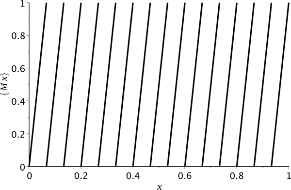
Many algorithms for generating pseudo-random numbers (PRNs for short) uniformly distributed in [0, 1] have the form of an iterative rule, ut+1 = F (ut), t = 0, 1, . . ., where both the range and the domain of the function F are [0, 1] and the initial seed u0 ∊ [0, 1] is given. Suppose that a sequence of PRNs {ut}t≥0 is generated by such a rule. Combine the numbers in pairs to obtain points (ut, ut−1) ∊ [0, 1]2, t = 1, 3, 5, . . . . On the one hand, these points are situated on the curve y = F(x). On the other hand, they have to be uniformly distributed in the unit square [0, 1]2 so the points will fill out the square without leaving gaps. Therefore, the plot of F should provide a sufficiently dense filling of the square. One example of a function that has such a property is the mapping y = {Mx}, where {x} denotes the fractional part of x, i.e., {x}=x−⌊x⌋, where ⌊⋅⌋ is the floor function, and M is a large positive number called a multiplier. The plot of y = {Mx} consists of parallel segments and the distance between them goes to zero as M → ∞ (see Figure 17.2).
(Voitishek and Mikhaĭlov (2006)). Consider the transformation y = {Mx + a} where {x} denotes the fractional part of x, and M ∊ Z and a ∊ ℝ are positive constants.
- If U ~ Unif(0, 1), then {MU + a} ~ Unif(0, 1).
- Let U0 ~ Unif(0, 1) and the sequence {Uk}k≥1 be generated from the rule Uk+1 = {MUk}. Then, Uk ~ Unif(0, 1) and Corr(U0, Uk) = Corr(Un, Un+k) = M−k for all n ≥ 0 and k ≥ 0.
Proof. First, we prove the fact that X := {MU} ~ Unif(0, 1). By the definition of the fractional part function, we have X ∊ [0, 1). Moreover, X = 0 iff MU is an integer what happens with probability zero. Hence ℙ(X ∊ (0, 1)) = 1. For x ∊ (0, 1), we have
ℙ(X≤x)=M−1∑k=0ℙ(k≤MU≤k+x)=M−1∑k=0ℙ(kM≤U≤kM+xM)=M−1∑k=0xM=x.
Here, we use the fact that 0 ≤ MU ≤ M and {z} ∊ [0, x] iff z∈∪k∈ℤ[k,k+x]. Thus, the CDF of X is FX(x) = x for x ∊ (0, 1). Therefore, X ~ Unif(0, 1).
Second, let us prove that {MU + a} ~ Unif(0, 1). Note that
{MU+a}={{MU}+{a}}d={U+b},
where b = {a} ∊ [0, 1). Show that ℙ({U + b} ≤ x) = x for x ∊ (0, 1). Consider two cases. (x ≤ b): Since {U + b} ≤ x iff 1 ≤ U + b ≤ 1 + x, we have
ℙ({U+b}≤x)=ℙ(1−b︸∈(0,1)≤U≤1+x−b︸∈(0,1))=(1+x−b)−(1−b)=x.
(b < x): Since {U + b} ≥ x iff x ≤ U + b ≤ 1, we have
ℙ({U+b}≥x)=ℙ(x−b︸∈(0,1)≤U≤1−b︸∈(0,1))=(1−b)−(x−b)=1−x.
Therefore, ℙ({U + b} ≤ x) = 1 − ℙ({U + b} ≥ x) = 1 − (1 − x) = x.
Finally, let us prove the last assertion. By induction, all Uk ~ Unif(0, 1), k = 0, 1, 2, . . . . Clearly, for any k ≥ 1, the pairs (Un, Un+k), n ≥ 0, all have the same distribution. Hence, we only need to prove that Corr(U0, Uk) = M−k for all k ≥ 0. Denote rk = Corr(U0, Uk). Let us show that rk=1Mrk−1fork≥1. Since r0 = Corr(U0, U0) = 1, the assertion will be proved by induction. A uniform random variable MU ~ Unif(0, M) can be expressed as a sum of its fractional and integer parts: MU=⌊MU⌋+{MU}. Clearly, ⌊MU⌋~Unif{0,1,...,M−1}(sinceℙ(⌊MU⌋)=k)=ℙ(MU∈[k,k+1))=1M for 0 ≤ k ≤ M − 1) and {MU} ~ Unif(0, 1) (as proved above). For any k = 0, 1, . . . , M − 1 and any x ∊ (0, 1), we have
ℙ(⌊MU⌋=k;{MU}≤x)=ℙ(MU∈[k;k+x])=xM=ℙ(⌊MU⌋=k)ℙ({MU}≤x).
Therefore, the fractional and integer parts are independent random variables. It is also true that E[⌊MU⌋]=(M−1)/2 and Var(⌊MU⌋)=(M2−1)/√12. Moreover, we have
U−E[U]√Var(U)=U−121√12=MU−M2M√12=⌊MU⌋+{MU}−(M−1)2−12M√12=√M2−1M2(⌊MU⌋−(M−1)2√(M2−1)12)+1M({MU}−121√12).
Now we are ready to calculate rk:
rk=Corr(U0,Uk)=√M2−1M2Corr(⌊MU0⌋,Uk)+1MCorr({MU0},Uk).
We proved that ⌊MU0⌋ and {MU0} = U1 are independent random variables. Moreover, since Uk = {MUk−1} = {M {MUk−2}} = · · · = g(U1) for some g : ℝ → ℝ, the random variable Uk as a function of U1 is independent of ⌊MU0⌋ as well. Thus, Corr(⌊MU0⌋,Uk)=0 and
rk=Corr(U0,Uk)=1MCorr({MU0},Uk)=1MCorr(U1,Uk)=1MCorr(U0,Uk−1)=1Mrk−1.
According to Proposition 17.5, a sequence {Ut, t = 0, 1, . . .} of random numbers uniformly distributed in (0, 1) can be generated from one random number U0 ~ Unif(0, 1) by using the rule Ut = {MUt−1} for t ≥ 1. We shall call this method a multiplicative method. Although the numbers obtained are dependent, the correlation between any two members of the sequence is negligible and rapidly goes to zero as the distance between the numbers in the sequence increases. Thus, the transformation y = {Mx + a} with a suitable choice of M and a can be used to generate pseudo-random numbers having good statistical properties such as uniformity and independence of samples. A drawback of the multiplicative method is that multidimensional tuples formed from the sequence {Ut}t≥0 lie on a family of multidimensional hyperplanes in the unit hypercube. For example, the points (U0, U1), (U2, U3), . . . lie on a family of M parallel lines.
The linear congruential generator (LCG) of PRNs is one of the oldest and simplest methods. It was proposed by Lehmer (1951). This algorithm is based on the mapping y = {Mx + a} but to avoid round-off errors the generating rule is written in a different form. As an example, let us consider the function y = {Mx} and suppose that x is a ratio of two integers: x=sm. Then,
{Msm}=Msm−⌊Msm⌋=Ms−⌊Msm⌋mm=Msmodmm.
The operation (s mod m) returns the remainder of an integer s after division by m:
smodm:=s−⌊s/m⌋⋅m
This operation is also called the reduction of s by modulo m; the result is called the residue of s modulo m.
The LCG works as follows. First, a sequence {st, t = 0, 1, . . .} of integers is generated. The initial number s0 (called the initial seed) is chosen by the user and all subsequent numbers are calculated from the rule
st=(Mst−1+a)modm,t=1,2,... (17.1)
By construction, all integers st lie between 0 and m − 1. Then, the pseudo-random numbers in [0, 1) are obtained by dividing these integers by m:
ut=stm,t=0,1,2,... (17.2)
The LCG is equivalent to the recurrence uk = {Mut−1 + a}, where all ut are of the form sm with integers s and m, but it avoids round-off errors. Here the multiplier M, the increment a, and the modulus m are integers so that 1 ≤ M < m, and 0 ≤ a < m. The initial seed s0 is an integer from {0, 1, . . . , m − 1}. If a = 0, then the generator is called a multiplicative congruential generator (MCG). It operates on multiplicative group of integers modulo m. The generating rule of the MCG is
st=Mst−1modm,ut=stm,t=1,2,... (17.3)
To guarantee that numbers produced from the rule (17.3) are all nonzero, the initial seed s0 has to be nonzero. Otherwise, all st = 0, t ≥ 1, if s0 = 0.
Construct PRNs generated by the LCG with M = 11, m = 16, a = 5, and s0 = 0.
Solution. The LCG rule is ut=st16, where st = (11st−1 + 5) mod 16. We first obtain the sequence of integers st, t ≥ 0:
S1=(11⋅0+5)mod 16=5mod 16=5,s2=(11⋅5+5)mod 16=60mod 16=12,s3=(11⋅12+5)mod 16=137mod 16=9,s4=(11⋅9+5)mod 16=104mod 16=8,s5=(11⋅8+5)mod 16=93mod 16=13,s6=(11⋅13+5)mod 16=148mod 16=4,s7=(11⋅4+5)mod 16=49mod 16=1,s8=(11⋅1+5)mod 16=16mod 16=0,s9=(11⋅0+5)mod 16=5mod 16=5,...
As is seen, the sequence obtained is periodic. The numbers repeat themselves after eight steps. The PRNs ut=stm,t≥0, are
0,516,1216,916,816,1316,416,116,0,516,...
The quality of the LCG depends on the choice of parameters M, a, and m. Often the modulus m is chosen as a prime number. Then, all calculations are done in the finite field Zm. Preferred moduli are Mersenne primes of the form 2r − 1, e.g., 231 − 1 = 2,147,483,647. Sometimes, m is a power of 2 since calculations can be done faster by exploiting the binary structure of computer arithmetic. Here are some choices of m and M for the MCG:
- m = 231 − 1 and M = 16807 (Park and Miller (1988));
- m = 240 and M = 517 (Ermakov and Mikhaĭlov (1982));
- m = 2128 and M = 5100109 mod 2128 (Dyadkin and Kenneth (2000)).
Since the set {0, 1, . . . , m − 1} is finite, the sequence generated by an LCG is periodic. That is, st+r = st holds for all t and some integer r > 0 called a period of the sequence. Let ℓ be the least possible period, which is called the length of period. Because there are only m possible different values of st, the maximum possible period of an LCG is m (or m − 1 if a = 0).
(Ermakov (1975)). The maximum possible length of period for the sequence st = Mst−1 mod 2p, t ≥ 1, with p ≥ 3 is ℓ = 2n−2. The maximum period length is achieved if M ≡ 3 mod 8 or M ≡ 5 mod 8 and the seed s0 is odd.
There are many ways of improving a classical linear congruential generator. Let us consider some of them (a more comprehensive review of modern PRNGs can be found in L’Ecuyer (2012)). To increase the maximum period, one can combine two (or more) LCG methods as follows. Let {ut(1)}t≥1 and {ut(2)}t≥1 be the outputs of two LCGs. A new sequence {ut}t≥1 is given by
ut:={u(1)t+u(2)t},t≥0.
Another generalization of the classical LCG is a multiple recursive generator defined by:
st=(M1st−1+⋯+Mkst−k)modm,ut=stm,t≥k,
where M1, . . . , Mk are multipliers selected from S:={0,1,...,m−1}; k ≥ 2 is the order of recursion, and (s0, s1, . . . , sk−1) is the seed sequence with si∈S for 0 ≤ i ≤ k − 1. The maximum period length for this generator is mk − 1.
One of important properties of the MCG is the ease of its parallelization. Suppose that a sequence {st}t≥0 is generated by (17.3). To share this sequence among several independent processors, we split it into several disjoint subsequences. This can be achevied by using different seeds situated far apart along the original sequence. The seeds s0(j), j ≥ 0, that start respective subsequences of length K are generated by using the leaping-frog generator:
s(j)0=As(j−1)0modm,wheres(0)0≡s0andA≡MKmodm.
Once the seeds are generated, the original generator (17.3) is used to obtain disjoint subsequences starting from these seeds:
s(j)t=Ms(j)t−1modm,u(j)t=s(j)tm,t=1,2,...,K,j≥0.
The maximum number of processors that can be served by such a leaping-frog generator cannot exceed the ratio ℓK of the length of period to the length of an individual subsequence.
17.3 Generation of Nonuniformly Distributed Random Numbers
Suppose that we have a good PRN generator for the uniform distribution Unif(0, 1). However, our ultimate goal is to be able to sample from any given probability distribution. This can be achieved by transforming uniform PRNs into nonuniform random numbers. We are interested in general transformation methods that work for large classes of distributions. The transformation methods should be fast and efficient and should not use too much memory. In the sequel we are going to consider three main groups of sampling algorithms, namely, inversion methods, composition methods, and acceptance-rejection methods.
17.3.1 Transformations of Random Variables
Recall that a (univariate) random variable defined on a probability space (Ω, ℱ, P) is a measurable function from Ω to ℝ. The support of X is defined as the smallest closed set S whose compliment Sc has probability zero: ℙ(X∈Sc)=0. The cumulative distribution function (CDF) of a random variable X is a function FX from ℝ to [0, 1] that is defined by FX(x) = ℙ(X ≤ x) for x ∊ ℝ. A CDF F satisfies the following properties:
- F is a nondecreasing, right-continuous (i.e., F (x+) = F (x)) function;
- F (−∞) = 0 and F (+∞) = 1.
A random variable X (and its CDF FX) is said to be
Discrete, if there exists a nonnegative function pX called a probability mass function (PMF for short) with a countable support such that
FX(x)=∑y≤x:pX(y)≠0pX(y)forx∈ℝ.
The CDF FX is a piecewise constant function with jumps.
(Absolutely) continuous, if there exists a nonnegative integrable function fX called a probability density function (PDF for short) such that
FX(x)=∫x−∞fX(x)dxforx∈ℝ.
The CDF FX is a continuous function (without jumps).
Since FX(∞) = 1, a PMF p satisfies ∑x∈Sp(x)=1, and a PDF f ≥ 0 satisfies ∫∞−∞f(x)dx=1. For a discrete random variable, the support is the smallest countable collection of points S so that ℙ(X∈S)=1. It is defined by S={x∈ℝ:pX(x)≠0}. Typically, the support S of a univariate continuous probability distribution is an interval of the real line. Since for a continuous random variable X the mass probability ℙ(X = x) is zero for any x ∊ ℝ, the support may be chosen to be an open interval.
Often, one random variable can be expressed as a function of another variate, say Y = f(X). Then sample values of Y can be obtained by applying the mapping f to sample values of X: yi = f(xi), i ≥ 1. Let us consider several useful examples.
A linear (or affine) mapping f(x) = α + βx. The density of Y = α + βX is given by fY(x)=1βfX(x−αβ). A normal random X ~ Norm(μ, σ2) can be expressed in terms of a standard normal variate Z ~ Norm(0, 1) as X = μ + σZ. Similarly, a uniform variable X ~ Unif(a, b) with a < b is a function of U ~ Unif(0, 1) given by X = a + (b − a)U.
A power mapping f(x) = xc for x > 0. Let X be a nonnegative random variable. The density of Y = Xc is then fY(x)=1cx1c−1f(x1c). For example, the density of Uc, where U ~ Unif(0, 1), is f(x)=1cx1c−1I(0,1)(x). A special case is a reciprocal of a nonzero variate: Y=1X. The PDF is fY(x)=1x2f(1x).
An exponential mapping f(x) = exp(x). The PDF of Y = eX is fY(x)=1xf(ln x) for x > 0. For example, the log-normal random variable is an exponential of a normal variate: Y = eμ+σZ, where Z ~ Norm(0, 1).
17.3.2 Inversion Method
The inversion method of generating nonuniform random numbers is based on the analytical or numerical inversion of the CDF. This method is most preferable if we wish to use it with low-discrepancy (quasi-random) sequences of numbers. Also it is compatible with some control variate techniques such as the antithetic variate method. The inversion method can be applied to both discrete and continuous distributions; however, its efficiency (in comparison with other methods) depends on how fast the inverse CDF can be evaluated.
17.3.2.1 Inverse Distribution Function
Consider a random variable X that has a continuous and strictly increasing on its support CDF F. Thus, the inverse function F−1 is well-defined and is also a strictly increasing function. Let us find the distribution function of Y := F(X). By using the definitions of a CDF and an inverse function, we obtain
FY(y)=ℙ(F(X)≤y)=ℙ(F−1(F(X))≤F−1(y))=ℙ(X≤F−1(y))=F(F−1(y))=y
for all y ∊ (0, 1). As is seen, the function FY is the CDF of a continuous random variable uniformly distributed on (0, 1). That is, F (X) ~ Unif(0, 1). This result provides us with a simple algorithm for sampling from continuous strictly increasing CDFs. Algorithm 17.1 is very simple and transparent. However, it relies on the knowledge of the inverse CDF F−1 in closed form (or the ability to compute F−1 in efficient manner). Figure 17.3 illustrates the method.
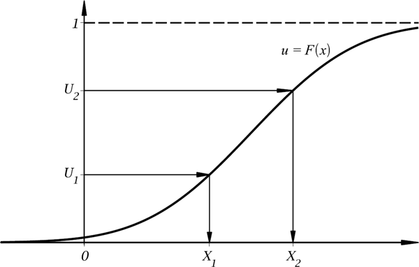
The Inverse CDF Method.
- (1) Obtain a draw u from the unform distribution Unif(0, 1).
- (2) A draw x from a CDF F is given by x = F−1(u).
Using the inverse CDF method, find generating formulae for
- (a) the uniform distribution Unif(a, b), a < b;
- (b) the exponential distribution Exp(λ), λ > 0;
- (c) the power distribution with the PDF f(x)=cxc−1I(0,1)(x),c>0;
- (d) the Weibull distribution with the PDF f(x)=αβxα−1e−xα/βIℝ+(x),α,β>0.
Solution.
- (a) The CDF of Unif(a, b) is F(x)=x−ab−a for x ∊ (a, b). Solve x−ab−a=u with u ∊ (0, 1) for x to find the inverse CDF: F−1(u) = a + (b − a)u. So the generating formula is X = a + (b − a)U.
- (b) The CDF of the exponential distribution with rate λ > 0 is F(x) = 1 − e−x, x > 0. Solve 1 − e−λx = u for x to obtain x=−1λln (1−u). If U ~ Unif(0, 1), then 1 − U ~ Unif(0, 1). So the generating formula for X ~ Exp(λ) simplifies: X=−ln Uλ.
(c) Integrate f(x)=cxc−1I(0,1)(x) on (0, x) for 0 < x < 1, to obtain
F(x)=∫x0f(x)dx=xc.
Thus, F−1(u) = u1/c and X = U1/c.
(d) The CDF is
F(x)=∫x0αβxα−1e−xα/βdx=1−e−xα/βforx>0.
Its inverse is F−1(u) = (−βln(1 − u))1/α. Thus, we obtain
X=F−1(1−U)=(−βlnU)1/α.
To generalize the inverse CDF sampling method to the case of any probability distribution, we define the generalized inverse CDF F−1 : (0; 1) → ℝ
F−1(u)=inf{x∈ℝ:u≤F(x)}. (17.4)
To justify this formula, let us consider two special cases. First, suppose that a CDF F of a random variable X has a jump discontinuity at x0, i.e., F(x0−) < F(x0). Therefore, ℙ(X = x0) = F(x0) − F(x0−) ≠ 0. The formula in (17.4) gives that
F−1(u)=x0forF(x0−)≤u≤F(x0),F−1(u)<x0foru<F(x0−),F−1(u)>x0foru>F(x0).
Thus, the random variable F−1(U) has a nonzero mass probability at x0 and
ℙ(F−1(U)=x0)=F(x0)−F(x0−)
as expected. Now, suppose that F has a flat section on [x0, x1] with x0 < x1. There exists u0 ∊ [0, 1] such that F(x) = u0 for x ∊ (x0, x1), F (x) ≤ u0 for x ≤ x0, and F(x) ≥ u0 for x ≥ x1. In this case, we have ℙ(x0 < X < x1) = F (x1−)−F (x0) = 0. Then, the generalized inverse has a jump at u0: F−1(u0−) ≤ x0 and F−1(u0) ≥ x1. Thus, with probability zero the random variable F−1(U) takes on a value in (x0, x1) as expected. Now, as we can see, the same sampling formula X = F−1(U), U ~ Unif(0, 1), with a generalized inverse CDF in (17.4), works for any CDF F , including those having a jump discontinuity or a flat section.
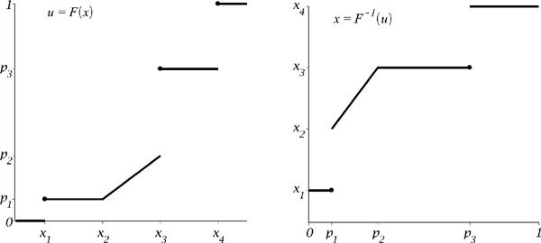
The plot of a CDF (the left plot) and its generalized inverse (the right plot). A mixture of a discrete distribution and a continuous distribution is considered. Note that a CDF is a right-continuous function and a generalized inverse CDF is a left-continuous function.
Using the inverse CDF method, find a generating formula for
- (a) a Bernoulli random variable X={0withprobability1−p,1withprobabilityp;
(b) a random variable with the PMF
f(x)=p1I{x1}(x)+p2I{x2}(x)+p3I{x3}(x),
where pi, i = 1, 2, 3, are positive probabilities so that p1 + p2 + p3 = 1.
Solution.
- (a) Sample U ~ Unif(0, 1). If U < p, then set X = 1; otherwise set X = 0. Verify that X has the Bernoulli distribution: ℙ(X = 1) = ℙ(U < p) = p and ℙ(X = 0) = ℙ(U ≥ p) = 1 − p.
(b) Suppose that x1 < x2 < x3. The CDF of X ~ f and the generalized inverse CDF are, respectively,
FX(x)={0ifx<x1,p1ifx1≤x<x2,p1+p2ifx2≤x<x3,1ifx3≤x,F−1X(u)={x1ifu≤p1,x2ifp1<u≤p1+p2,x3ifp1+p2<u,
for x ∊ ℝ and u ∊ (0, 1). Sample U ~ Unif(0, 1) and set
X=F−1X(U)={x1ifU≤p1,x3ifU>p1+p2,x2otherwise.
Justify the following method of sampling from the discrete uniform distribution on a set of N distinct numbers x1, x2, . . . , xN:
- (i) generate U ~ Unif(0, 1);
- (ii) set X = xK, where K=⌊N⋅U+1⌋.
Solution. We need to show that ℙ(X=xk)=1N for any k = 1, 2, . . . , N. Indeed,
ℙ(X=xk)=ℙ(⌊N⋅U+1⌋=k)=ℙ(k≤N⋅U+1<k+1)=ℙ(k−1N≤U<kN)=kN−k−1N=1N.
17.3.2.2 The Chop-Down Search Method
Consider a general discrete random variable with a countable support S={xj}j≥1 and mass probabilities {pj}j≥1, where pj = ℙ(X = xj) > 0 and Σj≥1pj = 1. The CDF F of such a discrete probability distribution is a piecewise-constant function. Let us assume that the mass points xj are sorted in increasing order: x1 < x2 < . . .. Then the CDF is given by F(x)=∑j:xj≤xpj. Hence the generalized inverse CDF is calculated as follows:
F−1(u)=inf{xk∈S:u≤k∑j=1pj}={xk∈S:k−1∑j=1pj<u≤k∑j=1pj} (17.5)
The requirement that mass points xj are sorted in increasing order is not necessary for the application of the inversion method. We can consider any arrangement for {xj}j≥1, since the sampling of X is equivalent to the sampling of a random index K∈ℕ with probabilities ℙ(K = j) = pj, j ≥ 1. First, generate U ~ Unif(0, 1). Second, find the index K ≥ 1 such that
K−1∑j=1pj<U≤K∑j=1pj. (17.6)
Finally, set X = xK. Note that the probability of the event that U satisfies the above double inequality is exactly pK. One of possible implementations of this approach is the chop-down search (CDS) algorithm (see Algorithm 17.2).
The number of cycles in the chop-down search method is equal to the expected value ∑j≥1jpj. Indeed, if U ∊ (0, p1], then the algorithm stops after one cycle, and this happens with probability p1 = ℙ(U ∊ (0, p1]). If U ∊ (p1, p1 + p2], then the algorithm stops after two cycles, and this happens with probability p2 = ℙ(U ∊ (p1, p1 +p2]), and so on. Let cU be the computational cost of the generation of one draw from Unif(0, 1) and cI the computational cost of one cycle of the method. Then, the total cost is
cU+cI∑j≥1jpj.
Algorithm 17.2 The Chop-Down Search (CDS) Method.
input: the mass points {xj}j≥1 and probabilities {pj}j≥1
generate U ← Unif(0, 1)
set K ← 0
repeat
set K ← K + 1
set U ← U − pK
until U ≤ 0
return X = xK
Find the computational cost of the CDS method for
- (a) the geometric distribution Geom(p) with ℙ(X = j) = (1 − p)j−1p, j ≥ 1, 0 < p < 1;
- (b) the Poisson distribution Pois(λ) with ℙ(X=j)=λjj!e−λ,j≥0,λ>0.
Solution. Compute the mathematical expectation ε=∑∞j=1jpj for both distributions. The total cost is then cU + CIε.
(a)ε=∞∑j=1j(1−p)j−1p=1p;(b)ε=∞∑j=0(j+1)λjj!e−λ=λ+1.
The computational cost can be reduced by rearranging elements of {(xj, pj)}j≥1. Consider an arrangement {ji}i≥1 of the integers 1, 2, 3, . . .. Then, the sequence {(xji,pji)}i≥1 defines another discrete probability distribution equivalent to the original one.
The computational cost of the chop-down search method attains its minimal value iff the mass probabilities are arranged in the decreasing order
p1≥p2≥p3≥⋯ (17.7)
Proof. Suppose that there exists another arrangement of the mass probabilities, {pj′}j≥1, for which (17.7) is violated and the expected value ε′=∑j≥1jp′j is minimal. There are two indices k and l, k < l, so that pl′ < pk′. Let us construct another arrangement {p″j}j≥1, which is obtained from {pj′}j≥1 by swapping pl′ and pk′, i.e., pl″ = pk′, pk″ = pl′, and pj″ = pj′ for j∉{k,l}. Let ε″=∑j≥1jp″j. We have
ε′−ε″=lp′l+kp′k−lp″l−kp″k=(l−k)(p′l−p′k)>0,
since l < k and pl′ < pk′. Hence ε″ < ε′. We arrive at a contradiction.
According to Proposition 17.7, the mass probabilities {pj}j≥1 should be arranged in decreasing order before applying the chop-down search method. Another way to speed up calculations is to use recurrence relations for mass probabilities. This allows us to reduce the parameter cI—the cost of one cycle of the CDS method. For example, the mass probabilities of a geometric random variable X ~ Geom(p) satisfy
ℙ(X=j+1)=ℙ(X=j)⋅(1−p),j=1,2,...
For a Poisson random variable X ~ Pois(λ), we have
ℙ(X=j)=ℙ(X=j−1)⋅λj,j=1,2,...
Algorithm 17.3 The Binary Search Method.
input: the mass points {xj}1≤j≤N and mass probabilities {pj}1≤j≤N
calculate F0 = 0, Fk=∑kj=1pj for 1 ≤ k ≤ N − 1, FN = 1.
generate U ← Unif(0, 1)
set L ← 0 and R ← N
repeat
set K←⌊L+R2⌋
if FK < U then
set L ← K
else
set R ← K
end if
until R = L
return X = xK
17.3.2.3 The Binomial Search Method
The formula (17.5) of the generalized inverse CDF requires the cumulative probabilities ∑kj=1pj,k≥1. Therefore, the inversion method can be speeded up if these cumulative probabilities are precalculated in advance and stored in memory. After that, to find K that satisfy (17.6), we can employ a fast search procedure such as the binary search method. Suppose that a random variable X takes on one of N distinct values x1 < x2 < · · · < xN with the respective mass probabilities p1, p2, . . . , pN , i.e., ℙ(X = xj) = pj, 1 ≤ j ≤ N. Note that a random variable with a countably infinite support can be reduced to the case with N mass points by suitable truncation of the support such that the total probability of removed mass points is very small. Suppose that N = 2r, then r = log2 N cycles are required to find K. For general N, the computation cost is proportional to ⌈log 2N⌉, where ⌈⋅⌉ denotes the ceiling function.
17.3.3 Composition Methods
It is a well-known fact that a linear combination (a mixture) of CDFs, PDFs, or PMFs with positive weights summing up to one is again a CDF, PDF, or PMF, respectively. The composition method aims to represent the probability distribution of interest as a mixture of simpler-organized distributions. The sampling from a mixture distribution is a two-step procedure. First, one of the distributions which appear in the composition is selected at random; second, a sample is drawn from the distribution selected (e.g., by using an inversion algorithm). In comparison with the inverse CDF method that requires one draw from Unif(0, 1), a composition method needs at least two uniform random numbers. However, the composition method allows us to express a probability distribution in a simpler form that allows for simplifying the sampling algorithm.
17.3.3.1 Mixture of PDFs
Consider a continuous random variable X with PDF f. Suppose that f can be represented as a linear combination of m PDFs f1, . . . , fm with m positive weights w1, . . . , wm so that w1 + · · · + wm = 1:
f(x)=m∑j=1wjfj(x),x∈ℝ.
The PDF f is called a mixture PDF. The support of f is a union of supports of fj, 1 ≤ j ≤ m. If all pairwise intersections of supports of fj are empty sets, then such a mixture is called a stratification.
Algorithm 17.4 The Composition Sampling Method.
input: {wj}j≥1 and {fj}j≥1
generate K from the probabilities ℙ(K = j) = wj, j ≥ 1
generate X from the PDF fK
return X
Proof of Algorithm 17.4. Let us find the distribution function of X generated by the algorithm. Applying the total probability law gives
ℙ(X≤x)=m∑j=1ℙ(X≤x;K=j)=m∑j=1ℙ(K=j)ℙ(X≤x|K=j)=m∑j=1wj∫x−∞fj(x)dx=∫x−∞m∑j=1wjfj(x)dx=∫x−∞f(x)dx=FX(x)
for all x ∊ ℝ.
Develop a stratification method for sampling from the PDF
f(x)={23xif0<x≤1,23if1<x<2,0otherwise.
Solution. As is seen, f is a piecewise linear function; it is constant on [1, 2] and linear on [0, 1]. Introduce two new PDFs: f1(x) ∝ for x ∊ (0, 1] and f2(x) ∝ 1 for x ∊ (1, 2). The second function is a PDF for Unif(1, 2). Hence, f2(x)=I(1,2)(x). Calculate a normalizing constant for f1 to obtain
f1(x)=x∫10xdxI(0,1](x)=2xI(0,1](x).
Now, the PDF f(x) can be decomposed as follows:
f(x)=23xI(0,1](x)+23I(1,2)(x)=13⋅(2xI(0,1](x))+23⋅I(1,2)(x)=13f1(x)+23f2(x):=w1f1(x)+w2f2(x).
Sampling from f2 is easy (see Example 17.3): X = 1 + U with U ~ Unif(0, 1). To sample from f1, we apply the inverse CDF method. First, find the CDF:
F1(x)=∫x0f1(x)dx=x2,x∈[0,1].
The inverse CDF is F−11(u)=√u,u∈[0,1]. As a result, we obtain the following sampling algorithm:
- (1) Generate two independent uniform random numbers U1, U2 ← Unif(0, 1).
- (2) Sample K ∊ {1, 2} as follows. If U1<13, then K = 1, else K = 2.
(3) Generate X from fK as follows:
- (i) if K = 1, then set X ← 1 + U2;
- (ii) if K = 2, then set X←√U2.
In general, the stratification method can be used with any partition of the support of a probability distribution. Suppose that A is the support of a PDF f. Let
A=m∪j=1Ak,wherei≠j⇒Ai∩Aj=ϕ.
Then, the PDF f admits the following representation:
f(x)=f(x)IA(x)=f(x)m∑j=1IAj(x)=m∑j=1wjfj(x),
where wj=∫Ajf(x)dx and fj(x)=1ωjf(x)IAj(x),1≤j≤m,x∈ℝ.
17.3.3.2 Randomized Gamma Distributions
Probability distributions whose PDFs contain special functions such as Bessel and other hypergeometric functions present a real challenge for sampling random numbers. By replacing a special function by its integral or series representation in terms of simpler functions, the PDF can be expressed as a mixture of more regular densities with known sampling algorithms.
For example, consider the noncentral chi-square distribution with κ > 0 degrees of freedom and noncentrality parameter λ > 0. Its PDF is
f(x;κ,λ)=12e−(x+λ)/2(xλ)κ4−12Iκ2−1(√λx),x>0. (17.8)
The modified Bessel function Iμ of the first kind (of order μ) admits the following series expansion:
Iμ(x)=(x2)μ∞∑j=0(x2/4)jj!Γ(μ+j+1).
By using this expansion for Iκ2−1 in (17.8), we can represent the noncentral chi-square PDF as a mixture of gamma densities with Poisson weights:
f(x;κ,λ)=12e−(x+λ)/2(xλ)κ4−12(√λx2)κ2−1∞∑j=0(λx/4)jj!Γ(κ2+j)=∞∑j=0e−λ/2(λ/2)jj!︸=pj(poissonprob.)12(x2)κ/2+j−1e−x/2Γ(κ2+j).︸=fj(x)(gammadensity) (17.9)
Recall that a random variable X is said to be gamma-distributed with shape parameter α and scale parameter θ, denoted by Gamma(α, θ), if its PDF is
fX(x)=θΓ(α)(θx)α−1e−θx,x>0. (17.10)
In (17.9), the PDF f(x; κ, λ) is expressed as a mixture ∑∞j=0pjfj(x), where {pj}j≥0 are mass probabilities of the Poisson distribution with intensity λ2 and fj is a gamma PDF of the form (17.10) with parameters α=κ2+j and θ=12 for all j = 0, 1, 2, . . . . Such a mixture probability distribution is called a randomized gamma distribution, denoted Gamma(Y1+κ2,12), where Y1~Pois(λ2).
In general, we can consider a mixture gamma distribution Gamma(Y + ν + 1, θ) with parameters ν > −1 and θ > 0, where the randomizer Y is a discrete random variable taking its values in the set of nonnegative integers with probabilities ℙ(Y = j) = pj, j = 0, 1, 2, . . . . The PDF f of such a randomized gamma distribution admits the form of a series expansion:
f(y)=∞∑j=0pjθΓ(v+j+1)(θy)v+je−θy.
Let us consider three choices for the randomizer Y. The resulting probability distributions are called the randomized gamma distribution of the first, second, and third types, respectively.
Let Y1 ~ Pois(α) be a Poisson random variable with mean α > 0. The randomized gamma distribution of the first type is Gamma(Y1 + ν + 1, θ) with the PDF
f1(y)=θ(θyα)v/2e−α−θyIv(2√αθy),y>0. (17.11)
So the noncentral chi-square distribution with parameters κ > 0 and λ > 0 is the randomized gamma distribution of the first type with ν=κ2−1,θ=12, and α=λ2.
A discrete random variable Y2 is said to have the Bessel probability distribution, denoted Bes(ν, b), with parameters ν > −1 and b > 0 if
ℙ(Y2=j)=(b/2)2j+vIv(b)j!Γ(j+v+1),j=0,1,2,... (17.12)
This distribution is related to many other distributions, where the modified Bessel function I is involved in the density, including the squared Bessel bridge distribution. The randomized gamma distribution of the second type is a mixture distribution Gamma(Y1 + 2Y2 + ν + 1; θ), where Y1~Pois(a+b4θ) and Y2~Bes(ν,√ab2θ) are independent Poisson and Bessel random variables, respectively. For any positive numbers θ, a, b, and ν > −1, the PDF is
f2(y)=θe−θy−(a+b)/(4θ)Iv(√ay)Iv(√by)Iv(√ab/(2θ)),y>0. (17.13)
A discrete random variate Y3 is said to follow an incomplete gamma probability distribution, which we simply denote by IΓ(ν, λ) with parameters λ > 0 and ν > 0, if
ℙ(Y3=j)=e−λλj+vΓ(j+v+1)Γ(v)γ(v,λ),j=0,1,2,..., (17.14)
where γ(a,x):=∫x0ta−1e−tdt is the lower incomplete gamma function. Note that if ν is a nonnegative integer, then the distribution of Y3 is simply a truncated and shifted Poisson distribution thanks to the property
γ(m,a)Γ(m)=1−(1+x+⋯+xm−1(m−1)!)e−x,m=0,1,2,...
We call a mixture probability distribution Gamma(Y3 + 1, θ), Y3 ~ IΓ(ν, λ), the randomized gamma distribution of the third type. The PDF is
f3(y)=θΓ(v)γ(v,λ)(θyλ)−v/2e−λ−θyIv(√4λθy),y>0. (17.15)
As we will see in the next chapter, randomized gamma distributions play a significant role in simulation of the so-called constant elasticity of variance diffusion model (see also Makarov and Glew (2010)).
17.3.3.3 The Alias Method by Walker
Let us study the case with discrete random variables. A mixture of PMFs is defined in the same manner as a mixture of PDFs. Consider m PMFs pj(x) and m weights wj > 0, 1 ≤ j ≤ m, such that w1 + w2 + · · · + wm = 1. The function p defined by p(x)=∑mj=1wjpj(x), x ∊ ℝ, is also a PMF called the mixture of the PMFs pj, 1 ≤ j ≤ m. To sample from p, we can apply Algorithm 17.4, where the sampling from the PDF fK is replaced by sampling from the PMF pK.
The alias method proposed by Walker (1977) allows us to represent any discrete probability distribution with m mass points S:={x1,x2,...,xm} as an equally weighted mixture of m two-point distributions. That is, there exist m two-point PMFs
pj(x)=qjI{xj}(x)+(1−qj)I{aj}(x)withaj∈Sandqj∈[0,1],1≤j≤m,
such that
p(x)=1mm∑j=1pj(x)forx∈ℝ. (17.16)
Since all weights in (17.16) are equal to 1m, Algorithm 17.4 is simplified and we obtain Algorithm 17.5.
Algorithm 17.5 The Alias Sampling Method.
input: m, {xj}1≤j≤m, {aj}1≤j≤m, and {qj}1≤j≤m
generate i.i.d. U1, U2 ← Unif(0, 1)
set K←⌊m⋅U1+1⌋
if U2 ≤ qK then
set X = xK
else
set X = aK
end if
return X
To obtain such a decomposition of the PMF p, we need to construct two lists, namely, the list of probabilities Q = (q1, q2, . . . , qm) and the list of aliases A = (a1, a2, . . . , am). This can be achieved by using the “leveling the histogram” procedure, which is described below. During this procedure the original histogram {wj = pj : 1 ≤ j ≤ m} is transformed into an equally weighed histogram {wj=1m:1≤j≤m}; the lists Q and A are generated in the course of this process.
Step 1: Start with wj = pj, qj = 1, and aj = xj for all j = 1, 2, . . . , m.
Step 2: Find two indices ℓ, u ∊ {1, 2, . . . , m} (ℓ and u stand for “lower” and “upper,” respectively) such that
wℓ=min1≤j≤m{wj}andwu=max1≤j≤m{wj}.
Step 3: If wℓ=wu=1m, then the histogram is levelled and the algorithm is stopped; otherwise (i.e., wℓ<1m<wu) we proceed with Step 4
Step 4: Set qℓ ← N wℓ and aℓ ← xu. Change wu←wu−(1m−wℓ) and wℓ←1m. Note that wu can become less than 1m. Go back to Step 2.
As is seen, the alias method requires at most m − 1 iterations until all columns of the histogram (i.e., the weights wj, 1 ≤ j ≤ m) become the same height.
Apply the alias method to the probability distribution with
p(x)=0.1I{1}(x)+0.2I{2}(x)+0.3I{3}(x)+0.4I{4}(x).
Solution. This is a four-point distribution with the list of mass points (x1, x2, x3, x4) = (1, 2, 3, 4) and the list of mass probabilities (p1, p2, p3, p4) = (0.1, 0.2, 0.3, 0.4). Initially, we set (a1, a2, a3, a4) = (1, 2, 3, 4) and (w1, w2, w3, w4) = (0.1, 0.2, 0.3, 0.4); all qi are equal to 1.
(i) The smallest weight is w1 = 0.1; the largest is w4 = 0.4. Set
w4←w4−(0.25−w1)=0.4−(0.25−0.1)=0.25,q1←4w1=0.4,w1←0.25,a1←x4=4.
(ii) Now, (w1, w2, w3, w4) = (0.25, 0.2, 0.3, 0.25). The smallest weight is w2 = 0.2; the largest is w3 = 0.3. Set
w3←w3−(0.25−w1)=0.3−(0.25−0.2)=0.25,q2←4w2=0.8,w2←0.25,a1←x3=3.
(iii) Now, (w1, w2, w3, w4) = (0.25, 0.25, 0.25, 0.25). All weights are equal to 0.25. Stop the algorithm.
As a result, we obtained the following two lists:
(a1,a2,a3,a4)=(4,3,3,4)and(q1,q2,q3,q4)=(0.4,0.8,1,1).
17.3.4 Acceptance-Rejection Methods
To generate realizations from some probability distribution, an acceptance-rejection method makes use of realizations of another random variable whose probability distribution is similar to the target one. The distribution from which the independent samples are generated is called a proposal distribution. Each sample can be accepted or rejected. The realizations being accepted have the target probability distribution. The computational cost of such a method is proportional to the average number of draws generated before one is accepted. Since the number of trials (draws) before the first success (acceptance of a draw) follows the geometric distribution, the average number of draws generated before an acceptance occurs is a reciprocal of the probability of the acceptance of a proposal draw.
Propose an acceptance-rejection method of sampling a point uniformly distributed in the circle C = {(x, y) : x2 + y2 ≤ 1}.
Solution. The circle C is contained in the square S = [−1, 1]2. To obtain a draw from the uniform distribution Unif(C), proceed as follows.
- (1) Sample a random point (X, Y) uniformly distributed in S as follows: X = 2U1 − 1 and Y = 2U2 − 1, where U1 and U2 are i.i.d. Unif(0, 1)-distributed random variables.
- (2) Accept the point if (X, Y) ∊ C, i.e., X2 + Y2 ≤ 1. Otherwise, the point is rejected and we return to (1).
The formal justification of this example and of the general acceptance-rejection method is based on Propositions 17.8–17.10, which follow.
Let a random vector X be uniformly distributed in a domain D ⊂ ℝd of a finite (d-dimensional) volume |D| < ∞. Let Ω be a subdomain of D. The distribution of X conditional on X ∊ Ω is uniform in Ω.
Proof. Let dΩ be an arbitrary subdomain of Ω. Then,
ℙ(X∈dΩ|X∈Ω)=ℙ(X∈dΩ;X∈Ω)ℙ(X∈Ω)=ℙ(X∈dΩ)ℙ(X∈Ω)=|dΩ|/|D||Ω|/|D|=|dΩ||Ω|.
Thus, the assertion is proved.
In Example 17.8 we deal with a case covered by Proposition 17.8. Proposed points are sampled uniformly on the square S. A point (X, Y) is accepted if it lies in the circle C. According to Proposition 17.8, the probability distribution of (X, Y) conditional on (X, Y) ∊ C is uniform in C. As a result, accepted points are uniformly distributed in C.
The simplest acceptance-rejection algorithm is the so-called Neumann method. Consider a bounded PDF f ≤ M with a support contained in a finite interval [a, b]. The plot of f on [a, b] is contained in the rectangle [a, b] × [0, M]. To sample from f we proceed as follows. First, sample (X, Y) uniformly in the rectangle [a, b] × [0, M]. This point is accepted if Y ≤ f(X) and rejected otherwise. According to Proposition 17.8, the distribution of accepted points is uniform in the region bounded by the plot of y = f(x) and the x-axis. Moreover, we can show that the distribution of the x-coordinate of an accepted point has the PDF f. That is, X conditional on Y ≤ f(X) has the distribution with the PDF f. This result will be proved in Proposition 17.9 in more general setting.
Consider a nonnegative integrable function g with support D ⊆ ℝd, that is, g(x) ≥ 0 for x ∊ D, g(x) = 0 for x ∉ D, and ID(g):=∫ℝng(x)dx=∫Dg(x)dx<∞ hold. The region
BD(g):={(x,y):x∈D,0<y<g(x)}⊆ℝd+1
is called the body of the function g.
Suppose that the (d + 1)-dimensional point (X, Y), with X ∊ ℝd and Y ∊ ℝ, is uniformly distributed in the body BD(g) of an integrable function g : D → [0, ∞) defined on D ⊆ ℝd. Then, the random vector X is distributed in D with the PDF proportional to g:
px(x)=1ID(g)g(x),x∈D.
Proof. The joint PDF of (X, Y) is
fX,Y(x,y)=1|BD(g)|IBD(g)(x,y)=1|BD(g)|ID(x)I(0,g(x))(y).
pX(x)=∫∞−∞fX,Y(x,y)dy=∫g(x)01|BD(g)|ID(x)dy=1ID(g)g(x)ID(x),
since ID(g) = |BD(g)|.
In the Neumann method the proposed sample values are drawn from the uniform PDF p(x)=1b−aI(a,b)(x). This choice is explained by the fact that the PDF p majorizes the target PDF f up to a multiplicative constant: f(x) ≤ C p(x) with C = M(b − a) (provided that f(x) ≤ M for all x ∊ [a, b]). A draw X is accepted if Y ≤ f(X) where Y ~ Unif(0, M). Therefore, the Neumann method can be generalized to the case with an arbitrary PDF f as long as we can find a majorizing function for f.
In what follows, we will require the following proposition that explains how to sample a point uniformly distributed in a body of a nonnegative function.
Let p be a multivariate PDF with support D. Suppose that X ~ p and (Y |X = x) ~ Unif(0, C p(x)) for some constant C > 0. Then, the point (X, Y) is uniformly distributed in the domain BD(C p).
Proof. The joint PDF of (X, Y) is
fX,Y(x,y)=fX(x)fY|X(y|x)=p(x)1Cp(x)I(0,Cp(x))(y)=1CID(x)I(0,Cp(x))(y)=1|BD(Cp)|IBD(Cp)(x),
since |BD(CP)|=∫DCp(x)dx=C∫Dp(x)dx=C..
Consider an n-variate PDF f with support D ⊆ ℝn. Suppose that there exists another PDF p called a proposal PDF and a constant C > 0 such that f(x) ≤ C p(x) for all x ∊ ℝn. Often p is chosen to be a simple function like a piecewise-linear function so that sampling from p is feasible.
Algorithm 17.6 The Acceptance-Rejection Method (Version 1).
- (1) Sample X from the proposal PDF p.
- (2) Generate U ~ Unif(0, 1) independent of X.
- (3) Accept X if U≤f(x)Cp(x). Otherwise return to (1).
The acceptance-rejection method can be visualized as choosing a subsequence of draws from a sequence of i.i.d. realizations from the PDF p in such a way that the resulting subsequence consists of i.i.d. realizations from the target PDF f.
i.i.d. draws from p |
˜X1 |
˜X2 |
˜X3 |
˜X4 |
˜X5 |
˜X6 |
. . . |
Accept? |
no |
yes |
no |
no |
yes |
yes |
. . . |
i.i.d. draws from f |
X1 |
X2 |
X2 |
. . . |
The proof of the acceptance-rejection method is based on Propositions 17.8–17.10. The steps of Algorithm 17.6 can be reformulated as follows. First, sample two random variables X ~ p and Y ~ Unif(0, C p(X)). As is proved in Proposition 17.10, the point (X, Y) is uniformly distributed in BD(C p). If (X, Y) ∊ BD(f), then this point is accepted. In accordance with Proposition 17.8, the accepted point is uniformly distributed in BD(f). Finally, as follows from Proposition 17.9, the X-coordinate is distributed with the PDF f.
While justifying Algorithm 17.6, we did not use the fact that f is a normalized PDF. The acceptance-rejection method is often applied to complicated multivariate densities only known up to a multiplicative constant. Thus, the following generalization of Algorithm 17.6 is quite useful in dealing with such cases. Consider the sampling from a PDF proportional to some nonnegative integrable function f. Suppose that there exists another integrable function g so that it majorizes f, i.e., f(x) ≤ g(x) for all x. Let f and g have the same support D. The sampling algorithm is as follows.
Algorithm 17.7 The Acceptance-Rejection Method (Version 2).
- (1) Sample X from the PDF p ∝ g, that is, p(x)=(∫ℝng(x)dx)−1g(x).
- (2) Generate U ~ Unif(0, 1) independent of X.
- (3) If U<f(X)g(X), then accept X, otherwise return to step 1.
A proposed draw X is accepted if the point (X, Y) being sampled uniformly in the body of g belongs to the body of f. Therefore, the probability of accepting X equals the ratio of the volumes of BD(f) and BD(g):
ℙ(Accept)=|BD(f)||BD(g)|=∫Df(x)dx∫Dg(x)dx.
To maximize this probability, we need to choose g as close to f as possible (see Figure 17.5). The average number of trials per one accepted draw (the computational cost of the acceptance-rejection method) is
Cost=ℙ(Accept)−1=∫Dg(x)dx∫Df(x)dx.

Develop an acceptance-rejection method for the PDF
f(x)=2arcinxπ−2,0<x<1.
Solution. By using the property that arcsin x≤π2xfor0<x<1, we obtain that
f(x)≤g(x):=ππ−2xfor0<x<1.
The ratio of f and g is arcsin x(π/2)x. The proposal PDF p ∝ g is given by p(x)=2xI(0,1)(x). The sampling algorithm is as follows.
- (1) Generate two i.i.d. U1, U2 ~ Unif(0, 1).
- (2) Sample X ~ p by using the inverse CDF method: X=√U1.
- (3) Accept X if U2≤arcsin X(π/2)X. Otherwise, return to (1).
Develop an acceptance-rejection method for the standard normal distribution using the double-exponential sampling distribution as a proposal one. Find the computational cost.
Solution. The standard normal PDF n is proportional to f(x)=e−x2/2. We have the following upper bound for f:
exp(−x22)=exp(−x2−2|x|+12−|x|+12)=exp(−(|x|−1)22)√ee−|x|≤√ee−|x|.
So the majorizing function is g(x)=√ee−|x|. Therefore, the proposal probability distribution is the double-exponential distribution with the PDF p(x)=12e−|x|, which can be expressed as a mixture:
p(x)=12e−xI[0,∞)(x)+12e−|x|I[−∞,0)(x).
To sample from p, we first obtain a draw from Exp(1) and then assign a random sign to it:
X={Ywithprobability12,−Ywithprobability12,whereY~Exp(1).
As a result, we obtain the following algorithm.
- (1) Generate three i.i.d. U1, U2, U1 ~ Unif(0, 1).
- (2) Sample X ~ p by using the composition method: X=sgn (U1−12)ln U2.
- (3) Accept X if U3≤f(X)g(X)=exp (−(|X|−1)22). Otherwise, return to (1).
The probability of acceptance PA is
PA=∫∞−∞e−x2/2dx√e∫∞−∞e−|x|dx=√2π2√e=√π2e≅0.7602.
Therefore, the computational cost is E[#trialsperacceptance]=1PA≅1.3155.
17.3.5 Multivariate Sampling
17.3.5.1 Sampling by Conditioning
A d-variate joint PDF fX of the random vector X = [X1, X2, . . . , Xd]⊤ can be represented as a product of univariate conditional densities:
fX(X)=fX1(x1)fX2|X1(x2|x1)⋯fXd|X1,...,Xd−1(xd|x1,...,xd−1),
where x = [x1, x2, . . . , xd]⊤. The sampling procedure is as follows:
Step 1. Generate X1~fX1.
Step 2. Generate X2 conditional on X1 from fX2|X1.
⋮
Step d. Generate Xd conditional on X1, . . . , Xd−1 from fXd|X1,...,Xd−1.
This method is simplified if the components Xj, 1 ≤ j ≤ d, are independent random variables. The joint PDF is then a product of marginal PDFs:
fX(X)=d∏j=1fXj(xj).
Construct a sampling algorithm for a random vector X uniformly distributed in a hyperparallelepiped D=∏dj=1(aj,bj),aj<bj,1≤j≤d.
Solution. The joint PDF is a product of d marginal uniform densities:
fX(X)=1|D|ID(X)=1(b1−a1)⋯(bd−ad)I(a1,b1)(x1)⋯I(ad,bd)(xd)=d∏j=11bj−ajI(aj,bj)(xj)≡d∏j=1fXj(xj).
Therefore, the vector X is formed of d i.i.d. uniformly distributed random variables:
Xj=aj+(bj−aj)Uj,Uj~Unif(0,1)1≤j≤d.
17.3.5.2 The Box–Müller method
A pair of independent standard normal random variables Z1 and Z2 can be generated from two independent Unif(0, 1)-distributed random variables by using the following steps.
(1) Define the random variables R and Θ implicitly by
Z1=RcosΘandZ2=RsinΘ. (17.17)
(2) One can show that R and Θ are independent random variables. Moreover, they can be simulated by the following formulae:
R=√−2lnU1andΘ=2πU2, (17.18)
where U1 and U2 are independent Unif(0, 1)-distributed random variables.
(3) Therefore, Z1 and Z2 can be expressed in terms of U1 and U2 as follows:
Z1=√−2lnU1cos(2πU2)andZ2=√−2lnU1sin(2πU2). (17.19)
To justify the Box–Müller method we apply the following theorem.
Theorem 17.11
(Bivariate Transformation Theorem, e.g., See Gut (2009)). Consider X and Y —jointly continuous random variables, and a one-to-one bivariate continuously differentiable transformation defined on the support of (X, Y) by u = g(x, y) and v = h(x, y). The joint PDF of U := g(X, Y) and V := h(X, Y) is fU,V(u,υ)=1|J(x,y)|fX,Y(x,y), where (x, y) is a unique solution to {g(x,y)=uh(x,y)=v and J(x, y) is the Jacobian determinant of the transformation defined by
J(x,y)=det[∂g∂x(x,y)∂g∂y(x,y)∂h∂x(x,y)∂h∂y(x,y)].
Since Z1 and Z2 are independent standard normal random variables, their joint PDF is
fZ1,Z1(z1,z2)=n(z1)n(z2)=12πe−12(z21+z22).
The bivariate transformation theorem allows us to obtain a joint PDF of the pair (R, Θ). The Jacobian determinant of the transformation in (17.17) is equal to r. Thus,
fZ1,Z2(rcosθ,rsinθ)=1rfR,Θ(r,θ)⇒fR,Θ(r,θ)=re−r2/212π,
for r > 0 and 0 < θ < 2π. The joint PDF of R and Θ is a product of the marginal PDFs fR(r)=re−r2/2I[0,∞)(r) and fΘ(θ)=12πI[0,2π)(θ). Therefore, R and Θ are independent random variable. Let us apply the inverse CDF method to generate R:
FR(r)=1−e−r2/2⇒R=F−1R(1−U1)=√−2lnU1,
where U1 ~ Unif(0, 1). Moreover, Θ ~ Unif(0, 2π), hence Θ = 2πU2 with U2 ~ Unif(0, 1). So, (17.18) is proved and (17.19) follows.
17.3.5.3 Simulation of Multivariate Normals
Consider a multivariate normal vector X = [X1, X2, . . . , Xd]⊤ ~ Normd(μ, Σ). If the covariance matrix Σ is a diagonal matrix diag (σ21,. . .,σ2d), then Xj, 1 ≤ j ≤ d, are all independent normals which can be expressed in terms of independent standard normal variables as follows:
Xj=μj+σjZj,Zj~Norm(0,1),1≤j≤d.
Independent standard normals can be generated by the Box–Müller method, by the acceptance-rejection method, or by the inverse CDF method. In the latter case we set Z=N−1(U) with U ~ Unif(0, 1), where the inverse normal CDF N−1(x) can be calculated numerically. One interesting application of standard normal random variables is the sampling of an isotropic vector in d dimensions.
- (1) Sample i.i.d. Z1, . . . , Zd ~ Norm(0, 1)
- (2) Define the vector X = [X1, X2, . . . , Xd]⊤ by Xj = Zj/Rd, 1 ≤ j ≤ d, where R2d=Z21+· · ·+Z2d. [Note that R2d is a chi-square random variable with d degrees of freedom.]
- (3) As a result, X is uniformly distributed on a unit d-dimensional sphere.
Suppose that the covariance matrix Σ has nonzero off-diagonal elements. Consider the following two general methods of sampling X:
- (1) using the Cholesky factorization of the covariance matrix;
- (2) using the conditional normal distribution.
Sampling by the Cholesky Factorization.
Let L be a lower-triangular matrix from the Cholesky factorization of Σ, i.e., Σ = L L⊤.
Let Z be a d-dimensional vector formed by i.i.d. standard normals Zj ~ Norm(0, 1), j = 1, 2, . . . , d. Then, we set
X:=μ+LZ~Normd(μ,Σ).
Conditional Normal.
Let us split the vector X into two parts:
X=[X1X2],whereX1∈ℝmandX2∈ℝd−m
for some 1 ≤ m < d. Split also the vector μ and matrix Σ to represent them in block form:
μ=[μ1μ2]andΣ=[Σ11Σ12Σ21Σ22],
where μ1 ∊ ℝm and μ2 ∊ ℝd−m are vectors; Σ11 ∊ ℝm×m, Σ12 ∊ ℝm×(d−m), Σ21 ∊ ℝ(d−m)×m, and Σ22 ∊ ℝ(d−m)×(d−m) are matrices. Then, the conditional distribution of X1 given the value of X2 is normal:
X1|{X2=x2}~Normm(μ1+Σ12Σ−122(X2−μ2),Σ11−Σ12Σ−122Σ21). (17.20)
Construct two methods of sampling from the trivariate normal distribution
Norm3([324],[900042023]),
using the Cholesky factorization and the conditional sampling approach, respectively.
Solution.
Find the Cholesky factorization of the covariance matrix. Let us solve the matrix equation Σ = L L⊤ to find L:
[900042023]=[ℓ1100ℓ21ℓ220ℓ31ℓ32ℓ33][ℓ11ℓ21ℓ310ℓ22ℓ3200ℓ33]⇒L=[30002001√2].
Thus, we obtain the following sampling formulae:
[X1X2X3]=[324]+[30002001√2][Z1Z2Z3]⇒{X1=3+3Z1,X2=2+2Z2,X3=4+Z2+√2Z3,
where Z1, Z2, Z3 are i.i.d. standard normals.
First, sample X1 ~ Norm(3, 9): X1 = 3 + 3Z1. Second, sample X2 conditional on X1. Recall that two normal variables are independent iff they are uncorrelated. Hence X2 is independent of X1 since Cov(X1, X2) = 0. Therefore, (X2|X1)d=X2~Norm(2,4) and X2 = 2 + 2Z2. Third, sample X3 conditional on X1 and X2. Again, X3 and X1 are uncorrelated, hence (X3|X1,X2)d=(X3|X2). We have
[X3X2]~Norm2([42],[3224])⇒X3|X2~Norm(3+X22,2).
Thus, we have X3=3+X22+√2Z3=4+Z2+√2Z3.
17.4 Simulation of Random Processes
A typical problem that requires simulation of sample paths of a stochastic process {X(t)}t≥0 is the estimation of a mathematical expectation of the form
E[g({X(t):0≤t≤T})] (17.21)
with some function g of an X-path. There are several possible cases.
The function g depends on a discretely monitored skeleton of the process X:
g=g(X(t1),X(t2)...,X(tm)),0≤t1<t2...<tm≤T.
One special case is when g = g(X(T)). For example, the estimation of E[g(X(T))] is required to price a European-style option.
- The function g depends on path-dependent quantities such as the running maximum/minimum of the process and the first passage time. It may be possible to sample such path-dependent quantities directly from their distributions rather than calculate them from a sample path.
- The function g depends on a full sample path of process X on [0, T]. Since it may be not feasible to generate a complete sample path of a continuous-time process (unless we deal with a Poisson process or a similar process with piecewise paths that changes at a finite number of time points), such a full path can only be obtained by applying an interpolation algorithm to a path skeleton.
So our goal is to sample a path skeleton
X(t1),X(t2),...,X(tm)for0≤t1<t2<⋯<tm≤T.
The skeleton can be generated from its exact multivariate distribution. In this case, the problem (17.21) can be reduced to the estimation of a multivariate integral of the form
∫Rmg(x1,x2,...,xm)fX(t1),X(t2),...,X(tm)(x1,x2,...,xm)dx1dx2⋯dxm
where f is a joint PDF of X(t1), X(t2), . . . , X(tm). Another approach is to sample an approximation path by applying some discretization scheme. Note that Brownian motion and other Gaussian processes as well as some jump processes can be sampled precisely form their path distributions. General diffusions can be simulated approximately by using, for example, the Euler approximation scheme.
17.4.1 Simulation of Brownian Processes
17.4.1.1 Sequential Sampling
The sequential sampling of Brownian motion (BM) and geometric Brownian motion is based on the property that Brownian increments on nonoverlapping intervals are independent. Consider a scaled Brownian motion with drift, W(μ,σ)x0(t):=x0+μt+σW(t). The standard BM is recovered from the process W(μ,σ)x0 if we take x0 = 0, μ = 0, and σ = 1. Suppose that the process W(μ,σ)x0 is to be sampled at a set of time points 0 = t0 < t1 < t2 < · · · < tm. For all j ≥ 1, we have
W(μ,σ)x0(tj)=x0+μtj+σW(tj)=W(μ,σ)x0(tj−1)+μ(tj−tj−1)+σ(W(tj)−W(tj−1)).
Since the increment W(tj) − W(tj−1) ~ Norm(0, tj − tj−1) is independent of W(μ,σ)x0(tj−1), we obtain the following simple algorithm.
Algorithm 17.8 Sequential Simulation of a Scaled BM with Drift.
input: x0, μ, σ, 0 = t0 < t1 < t2 < · · · < tm
set W(μ,σ)x0(0)=x0
for j from 1 to m do
generate Zj ← Norm(0, 1)
set W(μ,σ)x0(tj)←W(μ,σ)x0(tj−1)+μ(tj−tj−1)+σ√tj−tj−1Zj
end for
return {W(μ,σ)x0(tj)}0≤j≤m
The sample path of a geometric Brownian motion S(t)=S0eμt+σW(t)=eln S0+μt+σW(t) can be obtained by taking the exponential function of a sample path of the scaled BM with drift W(μ,σ)s0(t) that starts at x0 = ln S0, i.e., S(t)=exp (W(μ,σ)ln S0(t)).
Now we consider is a multidimensional BM W(t)=[W1(t),W2(t),...,Wd(t)]Τ. Each component of W(t) is a standard Brownian motion. Suppose that the processes Wj, 1 ≤ j ≤ d, are correlated. For 1 ≤ i, j ≤ d, the correlation coefficient between Wi(t) and Wj(t) is
ρij=Corr(Wi(t),Wj(t))=E[Wi(t)Wj(t)]−E[Wi(t)]E[Wj(t)]√E[W2i(t)]E[W2j(t)]=E[Wi(t)Wj(t)]t.
Let R = [ρij]1≤i,j≤d be the correlation matrix. R is a positive definite matrix with ones on the main diagonal. If we deal with independent Brownian motions then R = I. Apply the Cholesky factorization to find a lower triangular matrix L so that R = L L⊤. For example, for the two-dimensional case we have
R=[1ρ12ρ121]=LL⊺⇒L=[10ρ12√1−ρ12].
Algorithm 17.9 allows us to obtain a realization of W at time points t0, t1, . . . , tm with 0 = t0 < t1 < · · · < tm.
17.4.1.2 Bridge Sampling
Previously, we derived the probability distribution of Brownian motion pinned at the endpoints of a time interval. Recall that Brownian motion conditional on W (0) = a and W (T) = b is called a Brownian bridge from a to b on [0, T]. There exist several applications of the Brownian bridge. First, the bridge distribution can be used to refine a sample skeleton. Second, it can be used as an alternative to the sequential simulation method for sampling a Brownian trajectory.
Algorithm 17.9 Sequential Simulation of a Standard d-Dimensional BM.
input: L and 0 = t0 < t1 < t2 < · · · < tm
set W(0) = 0
for j from 1 to m do
generate d i.i.d. variates Zjt←Norm(0,1), 1 ≤ i ≤ d
set W(tj)←W(tj−1)+√tj−tj−1LZj, where Zj=[Zj1,Zj2,...,Zjd]Τ
end for
return {W(tj)}0≤j≤m
Suppose that a standard BM is sampled at m time moments 0 = t0 < t1 < · · · < tm = T and we wish to sample W (s) at some additional time moment s ∊ (0, T) conditional on these values. Let s ∊ (tj, tj+1) for some j ∊ {0, 1, . . . , m−1}. It follows from the Markov property of BM that
(W(s)|{W(ti)=xi,0≤i≤m})d=(W(s)|{W(tj)=xjW(tj+1)=xj+1}).
Hence W (s) can be sampled from the distribution of a Brownian bridge on [ti, tj+1]. By applying this procedure, a sample path can be refined without re-sampling its values at t1, t2, . . . , tm.
Consider the so-called dyadic partition of the time interval [0, T] with m = 2k points tj=jmT, where j = 0, 1, . . . , m and k ≥ 1. Let a realization of Brownian motion be sampled as follows:
Step1:sampleW(tm)conditionalonW(t0)=0,Step2:sampleW(tm/2)conditionalonW(t0),W(tm),Step3:sampleW(tm/4)conditionalonW(t0),W(tm/2),Step4:sampleW(t3m/4)conditionalonW(tm/2),W(tm),⋮Stepm:sampleW(tm−1)conditionalonW(tm−2),W(tm).
In other words, first we sample W(tm) and after that for each tj, 1 ≤ j ≤ m − 1, W(tj) is sampled conditionally on W (tℓ) and W(tk) previously generated, where the indices ℓ and k satisfy 0 ≤ ℓ < j < k ≤ m and j=ℓ+k2. As a result, a trajectory of BM is sampled at the time points in the following order of generation:
tm︸,tm/2︸,tm/4,t3m/4︸t2,t6,t10,...,tm−2︸,,tm/8,t3m/8,t5m/8,t7m/8,...︸t1,t3,...,tm−1︸ (17.22)
Bridge sampling with m = 8 time points is illustrated in Figure 17.6.

The bridge sampling algorithm is useful in pricing path-dependent financial instruments. Being applied with (randomized) low-discrepancy numbers, i.e., when the (randomized) quasi-Monte Carlo method is used, it allows us to reduce the variance of a path-dependent estimator. Another advantage is that the bridge sampling algorithm can be easily parallelized.
Algorithm 17.10 Brownian Bridge Sampling for a Dyadic Time Partition.
input: the time points tj=jmT,j=0,1, . . . , m, where m = 2k
generate Z ← Norm(0, 1)
set W(t0) ← 0, W(tm)←√TZ, and h ← T
for ℓ from 1 to k do
set h ← h/2
for j from 1 to 2ℓ−1 do
generate Z ← Norm(0, 1)
set W(t(2j−1)2k−ℓ)←12(W(t(j−1)2k−ℓ+1)+W(tj2k−ℓ+1))+√hZ
end for
end for
return {W(tj)}0≤j≤m
17.4.2 Simulation of Gaussian Processes
In accordance with the definition of a Gaussian process {X(t)}t≥0, for any sequence of time points 0 < t1 < t2 < · · · < tm, the vector X = [X(t1), X(t2), . . . , X(tm)]⊤ has a multivariate normal distribution Normm(μm, Σm) with
μm=[mX(t1)mX(t2)⋮mX(tm)]andΣm=[cX(t1,t1)cX(t1,t2)⋯cX(t1,tm)cX(t2,t1)cX(t2,t2)⋯cX(t2,tm)⋮⋮⋱⋮cX(tm,t1)cX(tm,t2)⋯cX(tm,tm)],
where mX(t) = E[X(t)] and cX(t, s) = Cov(X(t), X(s)) are, respectively, the mean and covariance functions. Therefore, the realization of X at time points t1, t2, . . . , tm can be constructed by sampling from the m-variate normal distribution Normm(μm, Σm) as follows.
(1) Apply the Cholesky factorization to find a lower-triangular matrix Lm so that
Σm=LmL⊺m.
- (2) Sample m i.i.d. standard normals Z1, Z2, . . . , Zm.
- (3) Set X = μm + Lm Z where Z = [Z1, Z2, . . . , Zm]⊤.
This generic algorithm can be applied to any Gaussian process including those listed below.
Brownian Motion W(μ,σ)x0(t):=x0+μt+σW(t) with m(t) = x0 + μt and c(t, s) = σ2 (tΛs) for s, t ≥ 0.
Itô Processes X(t):=∫t0μ(s)ds+∫t0σ(t)dW(S) with m(t)=∫t0μ(u)du and c(t,S)=∫t∧S0σ2(u)duforS,t≥0.
Fractional Brownian Motion W(H)(t) with c(t, s) = (t2H + s2H − |t − s|2H)/2 and m(t) = 0. Here, H ∊ [0, 1] is the so-called Hurst parameter. Note that W(1/2) is a standard BM with c(t, s) = (t + s − |t − s|)/2 = t Λ s for s, t ≥ 0.
Standard Brownian Bridge from a to b on [0, T], denoted {Ba,b[0,T](t)}0≤t≤T, with m(t)=a(T−t)+btT and c(t,s)=t∧s(T−t∨s)for0≤s,t≤T.
17.4.3 Diffusion Processes: Exact Simulation Methods
A diffusion process {X(t)}t≥0 is a solution to an initial value problem for a stochastic differential equation (SDE):
{dX(t)=μ(t,X(t))dt+σ(t,X(t))dW(t),t≥0,X(0)=X0. (17.23)
The process can also be written in the integral form
X(t)=X0+∫t0μ(s,X(s))ds+∫t0σ(s,X(s))dW(s). (17.24)
The functions μ and σ are called the drift coefficient and the diffusion coefficient, respectively.
The problem (17.23) (or (17.24)) can be solved analytically or numerically. One approach is to represent the process X as an explicit function of the underlying Brownian motion W :
X(t)=f(t,{W(s):0≤s≤t}). (17.25)
Such an explicit representation is called a strong solution to (17.23). As a result of (17.25), a sample path of the X-process is obtained by transforming a Brownian trajectory. Another approach is to find the transition PDF for X by solving the Kolmogorov equation. The strong solution and/or the transition density can be used to generate a realization of the diffusion X from its exact finite-dimensional distribution. As usual, our goal is to generate a path skeleton for an arbitrary sequence of time points. Alternatively, being unable to analytically solve (17.23), one can apply a numerical scheme to find an approximate realization of the diffusion process. The Euler scheme, which is the simplest and most popular simulation method, is considered in Section 17.4.4.
17.4.3.1 The Stochastic Calculus Approach
Most of the SDEs for which we can find a strong solution are SDEs with linear (w.r.t. the space variable) drift and diffusion coefficients. Let us consider some examples of such SDEs and derive transition probability distributions of their solutions.
Geometric Brownian motion is a solution to
dX(t)=μX(t)dt+σX(t)dW(t),X(0)=X0.
Applying the Itô formula gives X(t)=X0e(μ−σ2/2)t+σW(t). To model the transition X(s) → X(t) for 0 ≤ s < t, we use the following representation:
X(t)=X(s)e(μ−σ2/2)(t−s)+σ(W(t)−W(s))d=X(s)e(μ−σ2/2)(t−s)+σ√t−sZ,
where Z ~ Norm(0, 1) is independent of X(s).
-
dX(t)=μ(t)dt+σ(t)dW(t),X(0)=X0,
is a Gaussian process given by X(t)=X0+∫t0μ(u)du+∫t0σ(u)dW(u). By representing X(t) in terms of X(s) for 0 ≤ s < t and using the fact that the Itô integral ∫tSσ(u)dW(u) is normally distributed with mean 0 and variance ∫tSσ2(u)du, we obtain that the increments of X are normal:
Since the increments of X are independent, we are able to model the transition X(s) → X(t) for all 0 ≤ s < t.
The Ornstein–Uhlenbeck process is a solution to the SDE with a constant diffusion coefficient and linear drift:
The strong solution is
The conditional distribution of X(t) given X(s) for 0 ≤ s < t is normal:
17.4.3.2 The PDF Approach
Consider a Markov stochastic process {X(t)}t≥0 starting at X0 so that its transition PDF p given by p(s, t; y, x) dx = ℙ(X(t) ∊ dx | X(s) = y), 0 ≤ s < t, x, y ∊ ℝ, is known in closed form. Moreover, suppose that it is feasible to sample from the PDF p(s, t; y, ·). The general simulation algorithm is as follows.
Algorithm 17.11 Sequential Simulation of a Stochastic Process from Its Transition PDF.
input the PDF p, X0, 0 = t0 < t1 < t2 < · · · < tm
set X(0) = X0
for j = 1 → m do
generate X(tj) ← p(tj−1, tj; X(tj−1), x)
end for
return {X(tj)}0≤j≤m
For example, due to the time- and space-homogeneity property, the Brownian motion transition PDF p(s, t; y, x) reduces to a two-variable function p0 given by
as follows: p(s, t; y, x) = p0(t − s; x − y). The latter solves the PDE . To generate (W(tj)|{W(tj−1) = y}) ~ p(tj−1, tj; y, x) = p0(tj − tj−1; x − y), we first sample Z ~ Norm(0, 1) and then set .
To sample from a transition PDF, we can use a whole arsenal of sampling techniques such as the inversion method, composition approach, and acceptance-rejection technique. The main example considered in the current section is the exact simulation of a family of Bessel diffusions. We start with a squared Bessel (SQB) process and show that its transition PDF reduces to a randomized gamma distribution. Moreover, as demonstrated in Chapter 16, other processes such as the Cox–Ingersolll–Ross (CIR) process and the constant elasticity of variance (CEV) diffusion model can be obtained from the SQB process by means of a scale and time transformation and change of variable.
Let us consider a λ0-dimensional squared Bessel (SQB) process {X(t) ∊ ℝ+}t≥0 obeying the stochastic differential equation (SDE)
with constant parameters λ0 and ν > 0. For simplicity of presentation, we assume here that ν = 2. The process X is a time-homogeneous Markov process and its transition PDF is given by (16.15).
The transition PDF (16.15) looks very similar to the PDF (17.8) of the noncentral chi-square distribution. In fact, for the case when μ ≥ 0 or μ ∊ (−1, 0) and x = 0 is a reflecting boundary (so there is no absorption at the origin), the transition PDF p(t; y, x) of the SQB process reduces to the PDF f(x; κ, λ) in (17.8) as follows:
Following the composition method, the noncentral chi-square PDF (17.8) can be represented as a randomized gamma distribution (17.10). The value of X(t) conditional on X(s) = y has the randomized gamma distribution
for 0 ≤ s < t, y > 0. Therefore, we have the following sampling algorithm for the SQB process without absorption.
Algorithm 17.12 Sampling of an SQB Process without Absorption (Variant 1).
input X(0) = X0 > 0, 0 = t0 < t1 < · · · < tm, μ > −1
for j = 1 → m do
generate
generate X(tj) ← Gamma(Yj + μ + 1, 2(tj − tj−1))
end for
return {X(tj)}0≤j≤m
Now consider the case when μ < 0 and x = 0 is an exit or a killing boundary. The stochastic process X admits absorption at the origin. It can be shown that the transition PDF p given by (16.15) with does not integrate to one. Let us define the probability Psv of surviving before time t and the probability Pab of absorption before time t for the SQB process starting at x0 > 0:
The probabilities of surviving and absorption of the SQB process before time t are
respectively, where τ0 is the first hitting time (FHT) at zero. Here,
are, respectively, the lower and upper incomplete gamma functions.
Observe that the actual transition probability distribution is then a mixture of continuous and discrete probability distributions with the following generalized density:
for 0 ≤ s < t. Here, δ denotes the Dirac delta function that can be viewed as a generalized density of the discrete distribution with an only mass point at zero. With the probability Pab, the process is absorbed at zero. With the additional probability Psv, the process survives. The normalized transition PDF of the SQB process conditioned on the survival of the process before time t is
As is seen, the function on the right-hand side of (17.28) reduces to the form of (17.15) with ν = |μ|, λ = x0/(2t), and θ = 2t. Thus, the above normalized transition PDF follows the randomized gamma distribution of the third kind, Gamma(Y + 1, 2t), where Y ~ IΓ(|μ|, x0/(2t)). As a result, we obtain the following sampling algorithm that returns a sample path [X(t1), X(t2), . . . , X(tm)] and an approximation of the FHT τ0.
17.4.4 Diffusion Processes: Approximation Schemes
Approximation schemes can be used whenever an exact method is not available or not feasible. In particular, approximation methods are efficient for the numerical solution of multidimensional stochastic differential equations. Computational schemes for SDEs are based on the same ideas as the numerical methods for solving deterministic differential equations. A discrete-time approximation solution is calculated on a time grid with small time steps. To illustrate the main idea, let us first consider a Cauchy problem for a system of ordinary differential equations written in a vector form:
The solution admits the following integral representation on a small time interval [t, t + h]:
By applying a rectangle quadrature rule to the integral in (17.29), we derive the so-called Euler approximation scheme:
Algorithm 17.13 Sampling of an SQB Process with Absorption (Variant 2).
input X0 > 0, 0 = t0 < t1 < · · · < tm, μ < 0
set X(0) ← X0,
for j = 1 → m do
if then
set
generate Uj ← Unif(0, 1)
if Uj < pa then
end if
if then
generate
generate
else
set X(tj) ← 0
end if
end for
return {X(tj)}0≤j≤m and
A discrete-time numerical solution on the time grid {tk := kh}k=0,1,2,... is given by
The numerical solution approximates the genuine solution: ; it converges to the exact one as the time step h goes to zero. Applying a similar approach to stochastic differential equations, we can construct a discrete-time approximate realization (a skeleton) of a sample path. Since we deal with stochastic processes, there are different types of convergence of the numerical solution to the exact one.
17.4.4.1 Types of Convergence
Consider a continuous-time d-dimensional stochastic process {X(t)}t∊[0,T] and its discrete-time approximation defined on a time grid 0 = t0 < t1 < · · · < tm = T with the maximum step size h = max{tk − tk−1 : k = 1, 2, . . . , m}. The simplest time grid is an equally spaced grid with tk = kh with and k = 0, 1, . . . , m. Let us analyze the convergence of the approximate solution Xh to the genuine solution X, as h → ∞, in the Euclidian vector norm , where x = [x1, x2, . . . , xd]⊤ ∊ ℝd. We say that the approximation Xh has:
the strong order of convergence α > 0 if there exists C > 0 so that E
the mean-square order of convergence β > 0 if there exists C > 0 so that
the weak order of convergence γ > 0 if for any real-valued function f selected from some large class of functions (usually, f is a sufficiently smooth function) so that
17.4.4.2 The Euler Scheme
Consider a multivariate SDE
where W(t) is an d-dimensional standard Brownian motion with independent components, and a: ℝ × ℝd → ℝd and b: ℝ × ℝd → ℝd×d are, respectively, the drift and diffusion coefficient functions. The SDE (17.30) can be written in the integral form on [t, t + h], t ≥ 0, h > 0:
Application of the rectangular approximation formula to each integral in (17.31) gives
So, the Euler discrete-time approximation on a time grid 0 = t0 < t1 < · · · < tm = T is given by
where {Zk}k≥0 is a sequence of i.i.d. multivariate Normd(0, I)-distributed vectors.
Theorem 17.12
The Euler scheme has strong order and weak order 1. Moreover, the weak error admits the following expansion:
For a proof, see Kloeden and Platen (2011).
17.4.4.3 Extrapolation
The process of extrapolation uses two approximations computed from the same formula but with different step sizes to obtain higher-order approximation. The Richardson extrapolation method allows us to achieve second-order accuracy for a first-order scheme. For the Euler method with a constant time step h, we have
for some constant Cf that depends on f. Suppose that the number of steps m is even. Apply the Euler method with steps to obtain approximations and of the time-T realization X(T), respectively. By combining
we can eliminate the leading term of the error expansion:
The error of the combined estimate is of (weak) order 2. The variance of the combined estimator is
By making and positively correlated, we can reduce the variance. This can be achieved by using consistent Brownian increments in simulating paths of Xh and X2h. Suppose that is constructed from m i.i.d. normal vectors
The same normal increments can be used for sampling X2h. For example, to construct we use the normally distributed vectors
Here, the property that a sum of two normal random variables is again normally distributed is applied.
17.4.4.4 Error Analysis
Suppose that we wish to approximate some quantity Q by using a biased estimator Yh where h is a discretization parameter approaching zero. For example,
where Xh is the Euler approximation of a diffusion X and is a time step size. Introduce the approximation error ε(h) = Q − E[Yh]. Suppose that
holds for some positive constants C1 and β. Taking the logarithm of both parts of (17.34) gives
As is seen from the above equation, we can use the linear regression method to calculate C1 and β. First, we compute the sample estimate of Q for a decreasing sequence of values of h:
where are i.i.d. samples of and h1 > k2 > h3 > . . .. For example, we set hk = 2−k. Assuming that the number of draws, n, is sufficiently large so that the statistical error is negligible in comparison with the approximation error, we obtain
Now, we plot versus log hk for all hk and then perform a linear regression. As a result, the slope of the regression line gives us the order of approximation β.
In fact, the error includes two components: the approximation bias and the statistical (Monte Carlo) error. To optimize the method, it is helpful to separate these two errors:
Define the mean-square (statistical) error as
where is the sample estimator. The value of MSE(h, n) is
Here the constant C2 = Var(Y0+) is defined as the limiting value of the variance Var(Yh), as . To find the optimal values of the sample volume n and the discretization parameter h, we will minimize the computational cost for a given level of error: MSE = ε2. Clearly, the computational cost (i.e., the number of operations) is directly proportional to m and n. The number of steps is inversely proportional to h. Hence, the computational cost (or the runtime) is given by C3n/h, where C3 is another positive constant. Let us minimize the computational cost under the constraint that the mean-square error is fixed and equal to ε. The optimization problem takes the following form:
The problem (17.35) is easy to solve. As a result, we obtain that the computational cost is proportional to ε−2−1/β. Alternatively, we can solve the problem of minimizing MSE subject to a fixed computational cost s (see Exercise 17.23).
17.4.5 Simulation of Processes with Jumps
17.4.5.1 Poisson Processes
Recall that a Poisson process is a continuous-time stochastic process {Nλ(t)}t≥0 with independent, stationary, Poisson distributed increments that starts at zero. In other words,
- (a) Nλ(0) = 0;
- (b) for all m and 0 ≤ t0 ≤ t1 ≤ · · · ≤ tm, the increments Nλ(tk) − Nλ(tk−1), 1 ≤ k ≤ m, are independent random variables;
- (c) Nλ(t) − Nλ(s) ~ Pois(λ(t − s)) for 0 ≤ s < t.
The parameter λ is called the intensity of the process.
Every realization of a Poisson process is a step function that starts at the origin. It stays at each level k ≥ 0 for a random time period and then jumps to the next level k + 1. The occurrence time Tk is the time when the process jumps from k − 1 to k for k ≥ 1. Set τ1 = T1 and τk = Tk − Tk−1 for k ≥ 2. These variables {τk}k≥1 are called durations. We can express {Tk}k≥1 in terms of {τk}k≥1 as
Thus, a Poisson process can be defined via durations as follows:
A realization of a Poisson process can be generated from the sample values of the durations. The probability distribution of the random variables {τk}k≥1 is given by the following result.
Consider a Poisson process with occurrence times Tk, k ≥ 1, and durations τ1 = T1, τk = Tk − Tk−1, k ≥ 2. Then,
- (a) τk, k ≥ 1, are jointly independent, Exp(λ)-distributed random variables;
- (b) Tk ~ Gamma(k, λ), k ≥ 1.
For a complete proof of Propositions 17.13 and 17.14, see Gut (2009).
By using Proposition 17.13 and Equation 17.36, we come up with the following sampling algorithm of the Poisson process on [0, T].
Algorithm 17.14 Sampling a Poisson Process (Variant 1).
Input: λ > 0, T > 0.
- (1) Simulate i.i.d. τ1, τ2, . . . , τm ∊ Exp(λ) where m = sup{k : τ1 + · · · + τk ≤ T}.
- (2) Set .
- (3) Define .
Another algorithm for sampling a Poisson process is based on conditioning on the number of occurrences in a time interval. As it turns out, the joint distribution of the occurrence times conditional on the number of occurrences is the same as that of the order statistics of a sample from a uniform distribution.
The joint density of T1, T2, . . . , Tm conditional on Nλ(T) = m is
In other words,
where U(1), U(2), . . . , U(m) are the order statistics defined by sorting m i.i.d. Unif(0, T)-distributed random variables in increasing order.
Algorithms 17.14 and 17.15 allow us to sample a Poisson path on [0, T]. If we want to continue sampling on (T, T + T ′], T ′ > 0, then the sample path on [0, T] can be reused thanks to the following property.
If {N(t)}t≥0 is a Poisson process, then so are
- {N(t + s) − N(s)}t≥0 for every fixed s > 0;
- {N(t+Tk)−N(Tk)}t≥0 for every fixed k ≥ 1, where Tk is the time of the kth occurrence of the original Poisson process N.
This result, along with the property of independence of Poisson increments, allows us to simulate a Poisson process individually on disjoint intervals. Suppose we have generated the process Nλ on [0, T]. To continue the sample path on (T, T + T ′], we first generate another Poisson process independently of {Nλ(t)}t∊[0,T]. Second, we set for all t ∊ (T, T + T′].
The jumps of a Poisson process all have size one. A compound Poisson process is defined in such a way that the size of each of its jumps is random (see Section 16.2). Let Y1, Y2, . . . be i.i.d. random variables which are all independent of the Poisson process Nλ(t). A compound Poisson process with jump sizes Yk, k ≥ 1, is
The simulation of a compound Poisson process on [0, T] is straightforward. Applying Algorithm 17.14 or 17.15 gives us a sequence of occurrence times Tk, 1 ≤ k ≤ m, where m = Nλ(t) ~ Pois(λT). After that we set
Algorithm 17.15 Sampling a Poisson Process (Variant 2).
Input: λ > 0, T > 0.
- (1) Simulate Nλ(T) ~ Pois(λT). Set m = Nλ(T).
(2) Simulate i.i.d. U1, U2, . . . , Um ~ Unif(0, T). Sort them in increasing order:
- (3) Set Tk = U(k) for k = 1, 2, . . . , m.
- (4) Define .
17.4.5.2 Subordinated Processes
The variance gamma (VG) process is a three-parameter generalization of the Brownian motion model for the dynamics of the logarithm of the stock price. It is obtained by evaluating a scaled Brownian motion with drift at a random time given by a gamma process (see Madan and Seneta (1990)). The gamma process G(t; μ, υ) with mean rate μ > 0 and variance rate υ > 0 is a random process with independent gamma increments over nonoverlapping intervals of time.
The VG process X(t; σ, υ, θ) is defined in terms of the scaled Brownian motion with drift, B(t) ≡ W(θ,σ)(t) = θt + σW (t), and the gamma process with unit mean rate, denoted G(t) ≡ G(t; 1, υ), as
The PDF of the VG process at time t can be expressed as a normal density function conditional on the realization of the gamma time change. The risk-neutral process for the asset price is given by
where r and q are, respectively, the risk-neutral interest rate and dividend yield. The parameter ω = ln(1 − θυ − σ2υ/2)/υ is chosen so that the discounted asset price process e−(r−q)tS(t) is a true martingale.
Modelling of the variance gamma process relies on sampling from the normal and gamma probability distributions. One needs first to generate the gamma process and then to sample the Brownian motion conditional on the obtained values of the stochastic time process. Note that both the gamma process and Brownian motion are random processes with independent stationary increments. Thus, to sample a path of the variance gamma process at a discrete sequence 0 = t0 < t1 < t2 < · · · < tN, it is sufficient to generate the gamma increment G(ti) − G(ti−1) and then the Brownian increment B(gi) − B(gi−1) conditional on G(ti) = gi and G(ti−1) = gi−1 for all i = 1, 2, . . . , N. The sample values of G(ti) and X(ti) = B(G(ti)) can then be obtained by calculating cumulative sums of the respective increments. The increments of the gamma process G with mean rate one and variance rate θ and the Brownian process B with parameters θ and σ can be simulated as stated below:
G(t2) − G(t1) has the Gamma((t2 − t1)/θ,θ) distribution for any 0 < t1 < t2;
B(g2) − B(g1) has the Norm(μ(g2 − g1), σ2(g2 − g1)) distribution for any 0 < g1 < g2.
By repeating the above procedure n times and taking the cumulative sums of the increments, we can obtain the values of the variance gamma process at a discrete sequence of time moments. Algorithm 17.16 is used for sampling paths of the variance gamma process.
Algorithm 17.16 Simulation of the Gamma and Variance Gamma Processes.
input X0, 0 = t0 < t1 < t2 < · · · < tN , μ, σ, θ
G(0) ← 0
for k from 1 to N do
Δ Gk ~ Gamma((tk − tk−1)/θ,θ)
Δ Xk ~ Norm(μ ΔGk, σ2 ΔGk)
G(tk) ← G(tk−1) + ΔGk
X(tk) ← X(tk−1) + Δ Xk
end for
return {G(tk)}1≤k≤N and {X(tk)}1≤k≤N
17.5 Variance Reduction Methods
Consider the evaluation of a mathematical expectation E[h(X)], where h is a real-valued function of a random variable X having a PDF f. We call H ≡ h(X) a direct Monte Carlo estimator as opposed to an estimator with some variance reduction techniques embedded. The direct Monte Carlo sample estimator of E[h(X)] is
where {Xi}i≥1 are i.i.d. random variables with the common PDF f. A direct sample estimate is the following average with statistically independent realizations x1, x2, . . . , xn of X:
A large variance of the estimator h(X) results in slow convergence of the sample estimate to E[h(X)]. Any modification of the direct Monte Carlo method that results in a decrease of the variance is called a variance reduction method. One example of variance reduction techniques is the importance sampling method, which is discussed below. The goal of this section is to summarize various techniques used to improve the direct Monte Carlo method. Since a modification of the original estimator may result in an increase in computing time, we compare methods on the basis of their computational costs.
17.5.1 Numerical Integration by a Direct Monte Carlo Method
Consider a multidimensional integral . If the number of dimensions d is small (say, d ≤ 3) then deterministic quadrature rules can be successfully applied to evaluate I(g). For larger dimensions, it is more beneficial to use stochastic methods. As is pointed out in the beginning of this chapter, to apply the Monte Carlo method (MCM), the quantity of interest, say Q, needs to be represented in the form of a mathematical expectation of a random variable called the estimator of Q. Select a d-variate PDF f such that f(x) ≠ 0 if g(x) ≠ 0 for all x ∊ ℝd. If the integrand g has an integrable singularity at some point x0, then the PDF f should also be singular at x0 so that exists and is finite. Moreover, it is reasonable to select f having the same support as that of g. If the integral is taken on a manifold, e.g., a sphere, then the support of the PDF f has to be the same manifold. Rewrite the integral I(g) as follows:
where X ~ f; if g(x) ≠ 0 and g(x) ≠ ∞, h(x) := 0 if g(x) = 0, and . The integral I(g) = E[h(X)] is estimated by the Monte Carlo method as follows.
- (1) Generate n independent sample values drawn from the PDF f.
(2) Construct a sample estimate of the integral I(g):
(3) For 0 < α < 1, construct an asymptotically valid 100(1 − α)% confidence interval for I(g):
where is a sample variance for h(X), and zα/2 is a (1 − α/2)-quantile of the standard normal distribution.
As is seen, the Monte Carlo method allows us to simultaneously construct an approximation of I(g) and an upper bound for the error:
which is valid with confidence (1 − α)100%. The variance Var(h(X)) can be approximated by the sample variance . As is seen from (17.40), the approximation error is of order , as n → ∞. Since the number of sample values n is equal to the number of times the integrand g is evaluated, the Monte Carlo method can be compared with deterministic quadrature rules for which the approximation error is known in terms of n. For example, the midpoint quadrature rule provides the approximation error of order , as n → ∞. In contrast to the Monte Carlo method, the error of a quadrature rule depends the dimensionality d. The Monte Carlo method outperforms the midpoint rule for problems with d > 4. In general, the Monte Carlo method outperforms deterministic methods if d ≥ 10. For lower dimensionality (say, d ≤ 3), it is better to use a deterministic quadrature rule. For the case with 3 < d < 10, a combination of stochastic and deterministic methods may be a more efficient approach to computing the integral. The Monte Carlo method is said to beat the curse of dimensionality since its performance is not considerably affected by the dimensionality of the problem. Another advantage of the Monte Carlo method is that it can be applied to integrals of nonsmooth functions, whereas deterministic quadrature rules require the smoothness of higher-order derivatives of integrands.
The computational time required to calculate the estimate is a product of the number of samples, n, and the time tH required to calculate one sample value of H := h(X). Let δ be a given error level. Using (17.40), we obtain
Therefore, the total computational time tH · n is proportional to . The product tH ·Var(h(X)) is called the computational cost of the stochastic estimator h(X). Clearly, we can accelerate the Monte Carlo method by reducing the variance of the estimator. Another approach is to parallelize computations.
17.5.2 Importance Sampling Method
Clearly, there are many choices for the PDF f in (17.39) that fit for the estimation of I(g) by the Monte Carlo method. One obvious requirement on the density f is that it should include all singularities of the integrand to guarantee that the variance of the random estimator is finite. For example, let us estimate the value of the integral
by the Monte Carlo method. Consider the following two choices for the PDF f.
Choice 1: Let , i.e., X ~ Unif(0, 1). It is easy to verify that the variance of the random estimator is infinite.
Choice 2: Let for x ∊ (0, 1). Since f integrates to one, we set . Then, the random estimator
is bounded and hence has a finite variance.
Construct a Monte Carlo estimator of the integral
Solution. Notice that the integrand is a product of the function , which is a product of exponential PDFs, and the positive, bounded function (1 + x1 · · · x8)−2. Let us select the PDF
That is, the entries of the random vector X are independent exponentially distributed variables Xj ~ Exp(1), 1 ≤ j ≤ 8. Set the random estimator to be
To find an upper bound of Var(h(X)), use the following property (see Exercise 17.24). Suppose that Y is a bounded random variable such that 0 ≤ m1 ≤ Y ≤ m2 for some constants m1 and m2. Then,
Applying this property to Y = h(X) ∊ [0, 1], obtain that .
As is seen from the above examples, it is reasonable to select the PDF f as close to the integrand g as possible. This suggestion is confirmed by the importance sampling principle, which is presented just below. Since the computational cost is proportional to the variance of the estimator, the optimal PDF f solves the following optimization problem:
Let us prove that the variance attains its minimum value if f ∝ |g|. The proof is based on the Cauchy–Schwartz–Bunyakovsky inequality
for u, υ ∊ L2(ℝd) (here L2 is the set of square-integrable functions). Let us set and to obtain
Therefore, we obtain a lower bound of the variance
Now, it remains to show that the variance attains the lower bound when the PDF is proportional to |g|, that is, when with . Indeed, for , we have
In practice, it may be impossible to use the “best” PDF since the numerical evaluation of the normalizing constant c = I(|g|) is equivalent to the original problem. Alternatively, we can use an acceptance-rejection method that does not require the normalizing constant to be calculated. If sampling from f ∝ |g| is not feasible or is computationally expensive, then one can use any approximation PDF that is close to the optimal PDF. For example, a piecewise approximation of |g| can be used to construct the sampling density.
Approximate the integral by the Monte Carlo method where the sampling PDF is
- (a) (a constant approximation of g);
- (b) (a linear approximation of g).
Solution. Let us compare the variances of the random estimators with Xi ~ fi for i = 1, 2. We have
By using the PDF f2 instead of f1, we can reduce the computational cost by approximately times.
17.5.3 Change of Probability Measure
Let us consider another PDF such that for all x ∊ ℝ with f(x)h(x) ≠ 0. Apply the change of measure method to obtain:
where the last mathematical expectation in (17.44) is relative to . The weight function is called the likelihood function. According to the importance sampling method, the optimal PDF is proportional to the product f ·|g|. However, sampling from may not be feasible; therefore, one may use one of the following simple methods to “improve” the sampling density.
- (a) Shifting the PDF: for some c ∊ ℝ. The point c may be chosen in accordance with the maximum principle so that and f ·|g| attain their maximum at the same point. For example, consider a normal density f which reaches its maximum value at the mean μ. In this case, set c = ν − μ, where ν = arg max{f(x) · |g(x)|}.
- (b) Reshaping the PDF: for some c ∊ ℝ.
17.5.4 Control Variate Method
The main idea of the control variate method is to represent the unknown quantity as a sum of two parts. One part can be calculated analytically and the other part is to be estimated by the Monte Carlo method. Such a splitting is expected to decrease the variance. For example, consider the evaluation of . Suppose that there exists another function g0, which is close to g and for which the integral can be calculated analytically. Write I(g) = I(g0) + I(g − g0). To approximate the integral I(g − g0) we apply the Monte Carlo method with a PDF f:
If g0 is close to g, then the difference g − g0 is close to zero. So we expect that the Monte Carlo estimator of I(g − g0) has a smaller variance than that of the original integral I(g). Rewrite (17.45) as follows:
where and are, respectively, unbiased estimators of I(g) and I(g0).
Let us apply this method to the estimation of an arbitrary mathematical expectation Q = E[Y] of some random variable Y . Suppose that there exists another random variable Z with known mathematical expectation μZ such that Y and Z can be sampled simultaneously. Construct a new parametric family of random variables:
Clearly, the mathematical expectation of Y(b) is equal to Q for all b ∊ ℝ:
Thus, for every b ∊ ℝ, Y (b) is an unbiased estimator of Q. The random variable Z is called a control variate; Y (b), b ∊ ℝ, is called a controlled estimator. The sample estimate is constructed as usual.
Algorithm 17.17 The Control Variate Method.
(1) Generate n independent realizations (yj, zj), j = 1, 2, . . . , n.
(2) Set .
The optimal value of b chosen so that Var(Y (b)) reaches its minimum value is given by
The minimum variance of the controlled estimator is
Proof. The variance of the controlled estimator is a quadratic function of b:
Differentiate it with respect to b and equate the derivative obtained to zero:
Since the second derivative is positive, the variance attains its minimum value at the point bopt given by (17.47). The variance of the controlled estimator Y (b) for b = bopt is
Thus, Var(Y (bopt)) ≤ Var(Y) since 0 ≤ Corr(Y, Z)2 ≤ 1.
In practice, Var(Z) and/or Cov(Y, Z) are unknown in closed form. So, the optimal value of b can be approximated by the ratio of the sample covariance of Y and Z to the sample variance of Z. The variance reduction factor
increases very rapidly as |ρY Z| → 1, where ρY Z = Corr(Y, Z). For example, for , but if |ρ| = 0.99 then . This observation implies that a very high degree of correlation between the original estimator and a control variate is required to yield a substantial variance reduction.
If a nonoptimal value of b is used, then the controlled estimator may have a larger variance than the original one, as is demonstrated in the following example. Let Z be a control variate for Y so that . The controlled estimator Y (1) = Y − (Z − μZ) has a smaller variance than Y :
However, the variance of Y (−1) = Y + (Z − μZ) (i.e., replace Z by −Z) is larger than that of Y :
Apply the control variate method to the integral
Assume that a uniform sampling distribution is used in the direct Monte Carlo method. Calculate the variance reduction factor for the optimal control variate when d = 1, 5, 10.
Solution. The PDF of the uniform distribution in the unit hypercube (0, 1)d is . The direct estimator of the integral is Y = eU1+U2+···+Ud −1, where U1, U2, . . . , Ud are i.i.d. Unif(0, 1)-distributed random variables. Applying Taylor’s formula to the integrand gives us the following approximation: . Let us use Z = U1 + U2 + · · · + Ud as a control variate. The expected value of Z is
So, the controlled estimator is
To find the optimal value of b and the respective variance reduction, we calculate Cov(Y, Z), Var(Y), and Var(Z):
Therefore, the optimal value of b is . The results for d = 1, 5, 10 are summarized in Table 17.7. As is seen from the table, the efficiency of this control variate method is decreasing with the growth of d.
Efficiency of the control variate method.
d |
1 |
5 |
10 |
|---|---|---|---|
bopt |
1.69 |
14.73 |
220.71 |
Corr(Y, Z) |
99.18% |
91.38% |
82.02% |
Var(Y)/ Var(Y (bopt)) |
61.43 |
6.06 |
3.06 |
The above example suggests a universal approach to the construction of a control variate. Consider the estimation of Q = E[Y] with Y = h(X), X ~ f. Suppose that h: ℝ → ℝ has continuous derivatives and it can be approximated by the Taylor series expansion about x0:
Suppose that we are able to exactly calculate the moments E [(X − x0)j], 1 ≤ j ≤ k. Then, the random variable can be used as a control variate. The point x0 should be selected in a way such that | Corr(Y, Z)| is maximized.
17.5.5 Antithetic Variate
The antithetic variate method attempts to reduce the variance by exploiting a symmetry of a probability distribution. Consider the estimation of Q = E[h(U)], where U ~ Unif(0, 1). For example, with h(U) = (b − a)g(a + (b − a)U). Since U and 1 − U have the same distribution, the estimators h(U) and h(1 − U) are equally distributed as well. The antithetic estimator is defined as . Compare the variances of the direct estimator Y = h(U) and the antithetic estimator Yanti:
If h(U) and h(1 − U) are negatively correlated, then . Since every realization of Yanti requires two evaluations of h, the computational time is doubled when we apply the antithetic variate method. However, we can still expect a reduction in the computational cost if Var(Yanti) is less than Var(Y) by half. This is the case if h is a monotone function, as is proved in the following proposition.
Let h be a monotone function defined on [0, 1]; let Cov(h(U), h(1−U)), where U ~ Unif(0, 1), be finite. Then, Cov(h(U), h(1 − U)) ≤ 0.
Proof. Without loss of generality, assume that the function h is nondecreasing. We need to show that
Since h is nondecreasing on [0, 1], the value Q lies between the values of h at the endpoints on the unit interval, i.e., h(0) ≤ Q ≤ h(1). Consider the function defined on the unit interval, [0, 1]. The function f is zero at the endpoints, f(0) = f(1) = 0. Its derivative, f′(y) = h(1 − y) − Q, is a nonincreasing function. Since f′(0) = h(1) − Q ≥ 0 and f′(1) = h(0) − Q ≤ 0, the function f is nonnegative everywhere on [0, 1]. Therefore, . Integration by parts gives
Therefore, we have
Hence, .
In summary, the antithetic variate method attempts to reduce the variance by introducing negative correlation between pairs of realizations. Here are some examples of antithetic pairs.
- U and 1 − U are both Unif(0, 1)-distributed. Corr(U, 1 − U) = −1.
- Let F be a CDF and F−1 its generalized inverse. The random variables F−1(U) and F−1(1 − U) have the same CDF F , and they are antithetic to each other (F and F−1 are both monotone functions).
- Z and −Z are both standard normal variables, and Corr(Z, −Z) = −1.
- Z and 2μ − Z, where Z ~ Norm(μ, σ2), form an antithetic pair.
17.5.6 Conditional Sampling
Consider the estimation of E[h(X)] where h is a function of a random variable X. Suppose that there exists another random variable V correlated with X so that the conditional expectation can be calculated exactly. Applying the double expectation formula gives us
As is well known from a standard course on probability theory, for any pair of square-integrable random variables (Y, V), we have Var(Y) = E[Var(Y | V)] + Var(E[Y | V]). Setting Y = h(X) gives that
Therefore, using the estimator instead of h(X) always leads to a variance reduction.
Algorithm 17.18 The Conditional Sampling Method.
- (1) Generate n independent samples v1, v2, . . . , vn.
- (2) Calculate .
- (3) Estimate .
For this algorithm to be of practical use, the following conditions must be met.
- (a) It is easy to generate V .
- (b) E[h(X) | V = v] is readily computable for all v.
- (c) E[Var(h(X) | V)] is large relative to Var(E[h(X) | V]).
Let {Xi}i≥1 be i.i.d. random variables with a common CDF F; let R be a positive-integer-valued random variable independent of all Xi. Apply the conditional sampling method to estimate
Solution. We can try to improve the direct Monte Carlo estimator by isolating X1:
where the mathematical expectation is relative to X2, X3, . . . . Therefore,
where the external expectation is relative to R and the internal expectation is taken with respect to X2, X3, . . .. This method is efficient if ℙ(R = 1) is large.
17.5.7 Stratified Sampling
Stratified sampling is a special case of conditional sampling. Consider again the estimation of Q = E[h(X)]. We construct V such that Q = E[E[h(X) | V]] by stratifying the support of X as follows. Introduce mutually disjoint subsets A1, A2, . . . , Ak so that ℙ(X ∊ [Ui≥1Ai) = 1. Define a discrete random variable V ∊ {1, 2, . . . , k} so that V = i if X ∊ Ai, 1 ≤ i ≤ k. Set pi = ℙ(V = i) = ℙ(X ∊ Ai), 1 ≤ i ≤ k. The quantity of interest Q is given as a double expectation:
The stratified sample estimator of Q is
where are i.i.d. samples of X conditional on V = i, for 1 ≤ i ≤ k. The total sample size is n = n1 +n2 +· · ·+nk. A crucial assumption is that sampling of X conditional on V is possible. The variance of the stratified estimator is
where .
The most important question is how to select optimal allocation. The following two results provide a simple method and an optimal method for choosing the sample sizes ni, 1 ≤ i ≤ k, respectively.
Let the sample sizes ni be proportional to the probabilities pi, i.e., ni = n · pi, for i = 1, 2, . . . , k. Then, the variance of the stratified sample estimator does not exceed that of the direct sample estimator :
where n = n1 + n2 + · · · + nk.
Proof.
The optimal allocations are , which give
Proof. The proof is left as an exercise for the reader (see Exercise 17.35).
The standard deviations σi, 1 ≤ i ≤ k, are usually unknown. In practice, one may estimate them from “pilot” runs and then estimate the optimal sample sizes .
A typical problem where the stratified sampling method is efficient is numerical integration. Consider an integral of some function g on D ⊆ ℝd. Introduce a partition of D into k disjoint subdomains:
Apply the stratified sampling method to the integral to obtain
where V = i with probability for 1 ≤ i ≤ k, and is the conditional density of X given V = i for 1 ≤ i ≤ k.
Construct a direct sample estimator and a stratified sample estimator with two equal subintervals for the integral . Use 10 sample points for both estimators. Compare the variances of the estimators obtained.
Solution. Let us construct an estimator using a uniform sampling distribution, i.e., I = E[eU] with U ~ Unif(0, 1). The direct Monte Carlo estimator with n = 10 sample points is
where U1, . . . , U10 are i.i.d. Unif(0, 1)-distributed random variables. The variance of the direct MC estimator is
Divide the integration interval into two subintervals (k = 2): (0, 1) = (0,1/2) ∪ [1/2, 1). Now for each interval we need to find the conditional distribution of U and the probability, as is discussed above. The distribution of U ~ Unif(0, 1) conditional on {U ∊ (0, 1/2)} (or {U ∊ [1/2, 1)}) is uniform:
The probabilities are p1 = ℙ(U ∊ (0, 1/2)) = 1/2 and p2 = ℙ(U ∊ [1/2, 1)) = 1/2. Let n1 and n2 be sample sizes so that n1 + n2 = 10. The stratified sample estimator is
where and are i.i.d. U(0, 1)-distributed random variables. The variance of the stratified estimator is
If , then Var .
17.6 Exercises
- Exercise 17.1. In the “hit-or-miss” method, the value of π is estimated as follows. A point is sampled uniformly in the square [−1, 1] × [−1, 1], i.e., sample two independent Cartesian coordinates X, Y ~ Unif(−1, 1). A point (X, Y) is accepted if it lies inside the circle inscribed in the square, i.e., X2 + Y2 < 1. The experiment is repeated N times, and the number of accepted points, NH, is recorded. The ratio converges to a limiting value whose expression involves π.
- (a) Construct a random estimator of π based on the experiment described above.
- (b) Construct a sample estimate of π with N trials. Express it in terms of the ratio .
- (c) Construct a 99% confidence interval for π. Find the number of trials, N, required to obtain the confidence interval of length less than 10−3.
Exercise 17.2. Let U ~ Unif(0, 1) admit the following binary representation:
Show that the digits Bk, k = 1, 2, . . ., are independent Bernoulli random variables uniformly distributed in {0, 1}.
- Exercise 17.3. Propose an algorithm for simulating the occurrence of two dependent events A and B that uses only one uniform random variable U ~ Unif(0, 1). Assume that the probabilities ℙ(A) = pA, ℙ(B) = pB, and ℙ(A ∪ B) = q are given.
- Exercise 17.4. Using the inverse CDF method, find generating formulae for the following PDFs:
- Exercise 17.5. Using the inverse CDF method, find generating formulae for the Rayleigh distribution with the CDF F (x) = 1 − e−2x(x−b), x > b.
- Exercise 17.6. Let X be an absolutely continuous random variable such that the inverse function of its distribution function F is well-defined. Consider the problem of sampling X conditional on a < X < b, with F (a) < F (b).
- (a) Find the CDF for such a conditional distribution.
- (b) Show that the generating formula X = F−1(F (a) + (F(b) − F(a))U) with U ~ Unif(0, 1) produces the desired conditional distribution.
Exercise 17.7. Justify the following sampling formula for the geometric random variable X with parameter p ∊ (0, 1) (i.e., ℙ(X = k) = (1 − p)k−1p for k = 1, 2, . . .):
[Hint: Evaluate the probability ℙ(X = k), k = 1, 2, . . ..]
Exercise 17.8. Consider a random variable with the piecewise-constant PDF
Design a simulation algorithm using the inverse-transform method.
Exercise 17.9. Consider a random variable with a PDF f, which is proportional to the piecewise function
Find the constant c such that f(x) = cg(x) is a probability density. Design a simulation algorithm using the composition method.
Exercise 17.10. Present an acceptance-rejection method for a random variable on (0, 1) with the PDF of the form
Exercise 17.11. Construct the Neumann method (and estimate its computational cost) for sampling a random variable X whose density is proportional to
- (a) ;
- (b) f(u) = −u2 + 2 u + 3 , 0 < u < 3;
- (c) f(u) = u5/3 (1 − u)3/2, 0 ≤ u ≤ 1;
- (d) f(u) = u5/3 e−u, u > 0.
For each case, compute the probability of acceptance.
Exercise 17.12. Consider the triangular probability distribution with the PDF
- (a) Obtain the CDF F and then its inverse F−1. Describe the inverse CDF sampling method.
- (b) Develop the decomposition method using the strata {(0, 1], (1, 4)}.
(c) Determine which of the following majorizing functions provides the largest acceptance probability in the acceptance-rejection method:
Find the acceptance probability for each case.
- Exercise 17.13. Let X be a positive random variable with the probability density function , i.e., X = |Z| where Z ~ Norm(0, σ2). Develop an acceptance-rejection algorithm for generating a random variable from the PDF f using the exponential distribution Exp(λ) as the majorizing distribution. Which λ gives the largest acceptance probability (give the answer in terms of σ)?
Exercise 17.14. Consider a bivariate distribution with the joint density
- (a) Find the constant c.
- (b) Represent the joint density as a product of marginal and conditional univariate densities.
- (c) Construct the exact simulation algorithm based on the inverse CDF method. Consider the following approach: first model X and then Y.
Exercise 17.15. The density of a random variable X is represented in the integral form:
- (a) Show that fX is a density function.
(b) For the joint density
find a representation of the form fX,Y (u, v) = fY (υ)fX|Y (u|v).
(c) Based on the above representation of the marginal density
construct an algorithm for generating X, first by sampling Y from fY (υ), and then by sampling from the conditional density fX|Y (u|v).
- Exercise 17.16. Demonstrate how three independent tosses of a balanced coin can be modelled by two rolls of a balanced die (with six faces). In other words, develop an exact algorithm for sampling a vector [X1, X2, X3] formed by three independent discrete random variables uniformly distributed in {0, 1} by using two independent discrete random variables Y1 and Y2 uniformly distributed in {1, 2, 3, 4, 5, 6}.
- Exercise 17.17. Develop an algorithm that allows you to “replace” a fair roulette wheel (with 37 pockets numbered from 0 to 36) by a balanced die (with six faces labelled from 1 to 6). In other words, develop an exact algorithm for sampling a discrete random variable X uniformly distributed in {0, 1, 2, . . . , 36} by using a sequence (Yk)k≥0 of i.i.d. discrete random variables uniformly distributed in {1, 2, 3, 4, 5, 6}.
Exercise 17.81. Consider acceptance-rejection sampling from a standard normal distribution.
(a) Find the range for λ > 0 and c > 0 so that the function
majorizes .
- (b) Calculate the acceptance probability (as a function of c and λ).
- (c) Let us set and . Show that this choice of parameters maximizes the acceptance probability equal to .
(d) Show that the proposal CDF G is given by
(e) Develop computational algorithms
- (i) for sampling from the inverse of G;
- (ii) for sampling from the standard normal distribution by using the acceptance-rejection method with the proposal CDF G.
Exercise 17.19. Construct two methods of sampling from the trivariate normal distribution
using the Cholesky factorization and the conditional sampling approach, respectively.
Exercise 17.20. By applying the conditioning formula for a multivariate normal distribution, find the conditional (bridge) distribution of a Brownian motion with drift
In particular, show that for every 0 ≤ s < u < t, B(u) conditional on values of B(s) and B(t) has a normal distribution. Find the mean and variance of this conditional distribution.
Exercise 17.21. Consider a time-homogeneous random process {X(t)}t≥0 with the transition PDF p(t; y, x) defined by
with infinitesimally small dx. Using the notion of conditional probability, show that for every 0 ≤ t1 < t < t2 the bridge density b(t; x|t1, t2; x1, x2) of X(t) conditional on X(t1) = x1 and X(t2) = x2 is given by
Exercise 17.22. To simplify the Euler scheme, the Brownian increments ΔW = W (t + h) − W (t) can be replaced by other random variables with moments up to order 5 that are within of those of ΔW. Find the moments of the three point distribution
and compare them with those of ΔW.
Exercise 17.23. Solve the problem of minimizing the mean-square error subject to a computational budget s as follows:
where h is the discretization parameter, n is the sample size, and C1, C2, C3 are positive constants. Find the optimal values of h and n. Find the order (w.r.t. s) of the optimal MSE.
Exercise 17.24. Let a random variable Y satisfy 0 ≤ m1 ≤ Y ≤ m2 < ∞ a.s. Show that the variance of Y satisfies
[Hint: Consider .]
Exercise 17.25. Construct an importance sampling Monte Carlo method for evaluating the integral
Choose a nonconstant density function f so that it is close enough to the integrand and, on the other hand, can be easily sampled from.
- Exercise 17.26. Suppose that the integral dx is evaluated by the Monte Carlo method using the density f(x) ∞ (1 + cx), c > 0. Find the optimal value of c so that the variance of the standard estimator eX/f(X), X ~ f, attains its minimum value.
Exercise 17.27. Show the advantage of using the control variate method for evaluating the integral
Use the first two terms of a Taylor series of to construct the control variate.
Exercise 17.28. Let the integral dx be evaluated using the Monte Carlo method.
(a) Suppose that a combination of stratified random sampling and an antithetic variate method of the form
where f(x) = sin(πx/2), is applied to evaluate I = E[Y]. What is the efficiency gain of this estimator as compared to the direct Monte Carlo estimator X = f(U), U ~ Unif(0, 1).
- (b) How large a sample size do you need if you use the direct Monte Carlo or the antithetic stratified method of (a), respectively, in order to estimate the above integral, correct to four decimal places (i.e., the error does not exceed 10−4/2) with a confidence level of 95%?
Exercise 17.29. Suppose the integral
is approximated by the Monte Carlo method.
- (a) Find the variance of the direct Monte Carlo estimator X = 2f(U), U ~ Unif(0, 2), where f(x) = xm.
- (b) Suppose that a combination of stratified random sampling and an antithetic variate method of the form Y = f(U) + f(2 − U), U ~ Unif(0, 2), is applied to evaluate the integral.
- (i) Show that I = E[Y].
- (ii) Find the variance Var(Y).
- (iii) What is the efficiency gain of this estimator as compared to the direct estimator?
- (iv) How does the efficiency gain behave with the increase of m?
- (c) Suppose Z = U is used as a control variate. Give the formula of the controlled estimator. Find the variance reduction factor for the optimal controlled estimator in comparison with the direct Monte Carlo estimator. How does the efficiency gain behave with the increase of m? [Note: You are not required to compute the optimal value of the control variate parameter.]
- (d) How large a sample size do you need if you use the direct Monte Carlo or the control variate method of (c), respectively, to approximate the above integral, correct to two decimal places (i.e., the absolute error does not exceed 10−2/2) with a confidence level of 95%?
- Exercise 17.30. Let R ~ Geom(p), and X1, X2, . . . be i.i.d. Exp(λ) random variables. Find the distribution of .
Exercise 17.31. Construct an importance sampling Monte Carlo method for evaluating the integral
Choose the density function f so that it is close enough to the integrand and, on the other hand, can be easily sampled from. A constant density is not acceptable!
Exercise 17.32. Show the advantage of using the control variate method for evaluating the integral
Use u1 u2 · · · u5 to construct a control variate.
Exercise 17.33. Prove that for any pair of random variables (U, V),
[Hint: Use the fact that E[U2] = E[E[U2|V]] and Var(U) = E[U2] − (E[U])2.]
Exercise 17.34. Let X1, X2, . . . , Xn be independent random variables with expected values E[Xi] = μi and nonzero variances. Consider the following estimator of E[Y]:
Show that the values of c1, c2, . . . , cn that minimize Var(Z) are
Exercise 17.35. Show that the solution to the minimization problem
is given by
[Hint: Use Lagrange multipliers.]
Exercise 17.36. Show that the solution of
where g is a PDF, is given by
References
I. G. Dyadkin and G. H. Kenneth. A study of 128-bit multipliers for congruential pseudo-random number generators. Computer Physics Communications, 125(13):239–258, 2000.
S. M. Ermakov. Metod Monte-Karlo i smezhnye voprosy [The Monte Carlo Method and Related Questions]. Izdat. “Nauka,” Moscow, 1975. Second edition, augmented, Teoriya Veroyatnostei i Matematicheskaya Statistika. [Monographs in Probability and Mathematical Statistics].
S. M. Ermakov and G. A. Mikhaĭlov. Statisticheskoe modelirovanie [Statistical Modelling]. “Nauka”, Moscow, second edition, 1982.
A. Gut. An Intermediate Course in Probability. Springer Texts in Statistics. Springer, New York, second edition, 2009.
P. E. Kloeden and E. Platen. Numerical Solution of Stochastic Differential Equations. Applications of Mathematics. Springer, 2011.
P. L’Ecuyer. Random number generation. In Handbook of Computational Statistics, pages 35–71. Springer, 2012.
D. H. Lehmer. Mathematical methods in large-scale computing units. In Proceedings of a Second Symposium on Large-Scale Digital Calculating Machinery, 1949, pages 141–146, Cambridge, MA, 1951. Harvard University Press.
D. B. Madan and E. Seneta. The Variance Gamma model for share market returns. Journal of Business, 63(4):511–524, 1990.
R. N. Makarov and D. Glew. Exact simulation of Bessel diffusions. Monte Carlo Methods and Applications, 16(3):283–306, 2010.
S. K. Park and K. W. Miller. Random number generators: good ones are hard to find. Commun. ACM, 31(10):1192–1201, October 1988.
A. V. Voitishek and G. A. Mikhaĭlov. Numerical Statistical Modeling: Monte Carlo Methods. Akademiya, Moscow, 2006.
A. J. Walker. An efficient method for generating discrete random variables with general distributions. ACM Transactions on Mathematical Software, 3(3):253–256, 1977.