Chapter 8

General Multi-Asset Multi-Period Model

In this chapter we construct a general multi-asset discrete-time model with a finite state space. Most of the results of Chapter 5 and 7 will be generalized so that a single-period model and a binomial tree model become special cases of a more general framework.

8.1 Main Elements of the Model

Let us describe all main components of a general multi-period model defined on a filtered probability space $\left(\Omega ,ℱ,\mathbb{P},\mathbb{F}\right)$.

• There are T + 1 trading dates, t ∊{0, 1, 2,...,T}. Denote the collection of trading dates by T.
• A state space Ω = {ω1,ω2,...,ωM} represents all possible final states (or scenarios) of the world at time T.

• A filtration $\mathbb{F}={\left\{{ℱ}_t\right\}}_{t\in T}$ describes the arrival of information about the market with the passage of time:

  $\Omega ={ℱ}_0\subseteq {ℱ}_1\subseteq {ℱ}_2\subseteq ...\subseteq {ℱ}_T\equiv ℱ=2^{\Omega }.$

  For each date t ∊ T, the respective partition ${\mathcal{P}}_t$ of Ω that generates ℱt is given by

  ${\mathcal{P}}_t=\left\{A_t^1,A_t^2,...,A_t^{k_t}\right\}.\text{ (8.1)}$

  Here Atj, j =1, 2,...,kt, are atoms, and kt is the number of atoms of ${\mathcal{P}}_t$. The partitions form an information structure, i.e., ${\mathcal{P}}_{t-1}\preccurlyeq {\mathcal{P}}_t$ and for all t = 1, 2,...,T. Therefore, the numbers kt form an increasing sequence so that

  $1=k_0\le k_1\le ...\le k_T=M.$

• A probability measure ℙ on Ω describes the “real-world” probabilities for the possible states of the world, i.e., pj = ℙ(ωj) > 0 is the probability that the economy will be revealed to be in state ωj ∊ Ω at time T.

The information structure ${\left\{{\mathcal{P}}_t\right\}}_{t\in \text{T}}$ can be represented by a nonrecombining tree, where each node is an atom and two atoms are connected by an edge if one of the atoms is a subset of the other. We call it the information tree. Any final outcome ωj ∊ Ω is contained in the unique sequence of atoms, one from each partition ${\mathcal{P}}_t$:

$\left\{{\omega }^j\right\}=A_T^j\subseteq A_{T-1}^{j_{T-1}}\subseteq ...\subseteq A_1^{j_1}\subseteq A_0^1=\Omega ,$

where the indices jt ∊{1, 2,...,kt} depend on j. The sequence of atoms

$A_0^1\to A_1^{j_1}\to ...\to A_{T-1}^{j_{T-1}}\to A_T^j$

form a path in the information tree that goes from atom A01 = Ω to atom A = {ωTj}. Such a path uniquely represents ωj. A particular example of a three-period information tree is given in Figure 8.1.

The probability ℙ(ωj) can be computed as a product of conditional probabilities:

$\begin{array}{ll}\mathbb{P}\left({\omega }^j\right)\hfill & =\mathbb{P}\left(\left\{{\omega }^j\right\}|A_{T-1}^{j_{T-1}}\right)\cdot \mathbb{P}\left(A_{T-1}^{j_{T-1}}\right)\hfill \\ \hfill & =\mathbb{P}\left(\left\{{\omega }^j\right\}|A_{T-1}^{j_{T-1}}\right)\cdot \mathbb{P}\left(A_{T-1}^{j_{T-1}}|A_{T-2}^{j_{T-2}}\right)\cdot \mathbb{P}\left(A_{T-2}^{j_{T-2}}\right)\hfill \\ \hfill & ⋮\hfill \\ \hfill & =\mathbb{P}\left(\left\{{\omega }^j\right\}|A_{T-1}^{j_{T-1}}\right)\cdot \mathbb{P}\left(A_{T-1}^{j_{T-1}}|A_{T-2}^{j_{T-2}}\right)\cdots \mathbb{P}\left(A_2^{j_2}|A_1^{j_1}\right)\cdot \mathbb{P}\left(A_1^{j_1}\right).\hfill \end{array}\text{ (8.2)}$

Therefore, we may refer to ℙ(ωj) as a path probability. Equation (8.2) gives us another method of constructing the probability measure ℙ. We only need to define the conditional probability ℙ(At+1 | At) for every pair of atoms $A_t\in {\mathcal{P}}_t$ and $A_{t+1}\in {\mathcal{P}}_{t+1}$ with the property At+1 ⊆ At.

For calculating derivative prices at an intermediate time t ∊ T we need conditional expectations of the form Et[X] ≡ E[X |ℱt] (where X :Ω → ℝ is a random variable). The σ-algebra ℱt is generated by the partition ${\mathcal{P}}_t$ with kt atoms, as given in (8.1). Therefore, the conditional expectation Et[X] is a random variable that is constant on atoms of ℱt; it is given by

${\text{E}}_t\left[X\right]\left(\omega \right)={\displaystyle \sum _{i=1}^{k_t}\text{E}\left[X|A_t^i\right]}{\mathbb{I}}_{A_t^i}\left(\omega \right).$

The conditional expectation of X given atom Ati is calculated as follows:

$\text{E}\left[X|A_t^i\right]=\frac{\text{E}\left[X{\mathbb{I}}_{A_t^i}\right]}{\mathbb{P}\left(A_t^i\right)}=\frac{1}{\mathbb{P}\left(A_t^i\right)}{\displaystyle \sum _{\omega \in A_t^i}X\left(\omega \right)\mathbb{P}\left(\omega \right),i=1,2,...,k_t.}$

For each state ωj ∊ Ati, we can find a unique sequence of atoms

$\left\{{\omega }^j\right\}=A_T^j\subseteq A_{T-1}^{j_{T-1}}\subseteq ...\subseteq A_{t+1}^{j_{t+1}}\subseteq A_t^i.$

Thus, the probability of state ωj can be calculated as follows:

$\mathbb{P}\left({\omega }^j\right)=\mathbb{P}\left(\left\{{\omega }^j\right\}|A_{T-1}^{j_{T-1}}\right)\mathbb{P}\left(A_{T-1}^{j_{T-1}}|A_{T-2}^{j_{T-2}}\right)...\mathbb{P}\left(A_{t+1}^{j_{t+1}}|A_t^i\right)\mathbb{P}\left(A_t^i\right).$

As a result, we can simplify the formula of the conditional expectation to obtain

$\text{E}\left[X|A_t^i\right]={\displaystyle \sum _{\omega \in A_t^i}X\left(\omega \right)\mathbb{P}\left(\left\{{\omega }^j\right\}|A_{T-1}^{j_{T-1}}\right)\mathbb{P}\left(A_{T-1}^{j_{T-1}}|A_{t-2}^{j_{T-2}}\right)...\mathbb{P}\left(A_{t+1}^{j_{t+1}}|A_t^i\right).}$

In conclusion, let us consider several examples of multi-asset multi-period models.

Example 8.1.

Clearly, the standard binomial lattice model fits the definition of a general multi-period model. The state space Ω is the collection of M = 2T distinct paths in the recombining binomial tree with T periods, where each path is coded by a sequence of the letters D's and U's (of length T). That is, ω = ω1ω2 ...ωT, where each ωt ∊{D, U} is the time-t market move. The partition ${\mathcal{P}}_t$ consists of 2t atoms. Each atom of ${\mathcal{P}}_t$ contains 2T−t paths, all having identical first t market moves. The probability measure ℙ on Ω is defined by the probability p ∊ (0, 1) of a single upward move U. The probability of scenario ω ∊ Ω is found to be

$\mathbb{P}\left(\omega \right)=p^{\#\text{U}\left(\omega \right)}{\left(1-p\right)}^{\#D\left(\omega \right)}.$

Select an atom $A_t\in {\mathcal{P}}_t$ so that ω ∊ At iff ${\omega }_1,...,{\omega }_t={\overline{\omega }}_t$ for some ${\overline{\omega }}_1,...,{\overline{\omega }}_t$ ∊{D, U}. That is, $A_t=A_{{\overline{\omega }}_1...{\overline{\omega }}_t}$. This atom is a subset of $A_{{\overline{\omega }}_1...{\overline{\omega }}_{t-1}}\in {\mathcal{P}}_{t-1}$. The conditional probability of $A_{{\overline{\omega }}_1...{\overline{\omega }}_t}$ given $A_{{\overline{\omega }}_1...{\overline{\omega }}_{t-1}}$ is

$\mathbb{P}\left(A_{{\overline{\omega }}_1...{\overline{\omega }}_t}|A_{{\overline{\omega }}_1...{\overline{\omega }}_{t-1}}\right)=p^{\#\text{U}\left({\overline{\omega }}_t\right)}{\left(1-p\right)}^{\#\text{D}\left({\overline{\omega }}_t\right)}.$

Therefore, the probability of an individual scenario ω ∊ Ω is computed as

$\mathbb{P}\left(\omega \right)=p^{\#\text{U}\left(\omega \right)}{\left(1-p\right)}^{\#\text{D}\left(\omega \right)}.$

Example 8.2.

A generalization of the binomial tree model is a multinomial tree model, where at each time moment there exist n ≥ 2 possible continuations denoted by Mj for j = 1, 2,...,n. Note that for a binomial model we use D ≡ M1 and U ≡ M2. A scenario in this model is a path in a nonrecombining n-nomial tree with T periods. Each path can be coded by a sequence of length T formed from the symbols M1, M2,..., Mn:

$\Omega =\left\{{\omega }_1{\omega }_2...{\omega }_T:{\omega }_1,{\omega }_2,...,{\omega }_T\in \left\{{\text{M}}_1,{\text{M}}_2,...,{\text{M}}_n\right\}\right\}.$

Clearly, the state space Ω has M = nT possible scenarios. The probability measure ℙ is defined by the collection of probabilities pi ∊ (0, 1), i = 1, 2,...,n, in which pi is the probability of the single move Mi. Let #Mi(ω) give the number of Mi in the sequence ω. The probability of ω ∊ Ω is computed as

$\mathbb{P}\left(\omega \right)=p_1^{\#{\text{M}}_1\left(\omega \right)}{p}_2^{\#{\text{M}}_2\left(\omega \right)}...p_n^{\#{\text{M}}_n\left(\omega \right)}.$

Example 8.3.

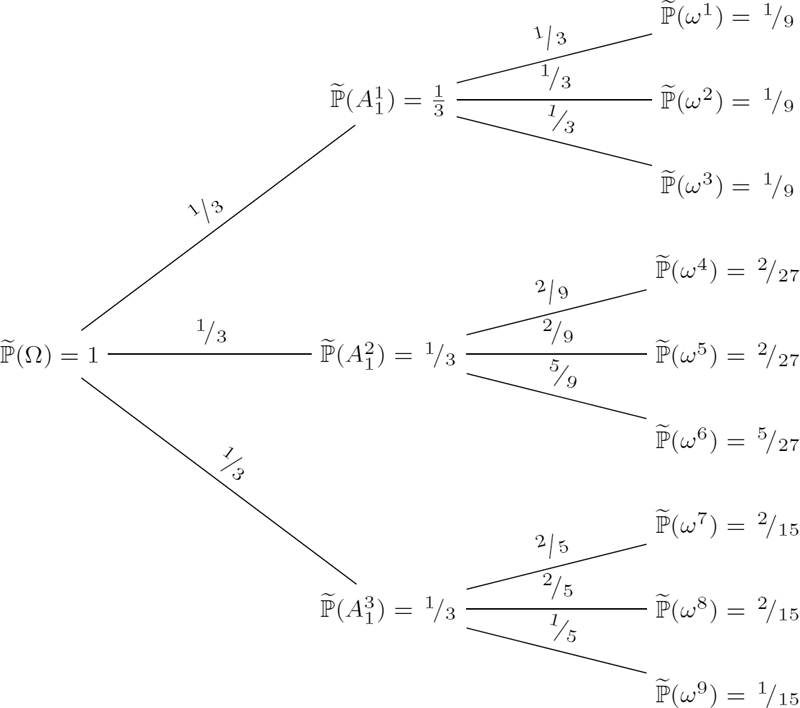
Consider a two-period trinomial model. Assume that by the end of period one the economy can end up in one of three possible scenarios. Moreover, for each of these possibilities, there are three alternative continuations throughout period two. Therefore, in total there are nine possible states of the world (M = 9) at time T = 2. The filtration $\mathbb{F}={\left\{{ℱ}_t\right\}}_{t\in \left\{0,1,2\right\}}$ is generated by the information structure ${\mathcal{P}}_0\preccurlyeq {\mathcal{P}}_1\preccurlyeq {\mathcal{P}}_2$ with the following partitions:

$\begin{array}{ll}{\mathcal{P}}_0\hfill & =\left\{A_0^1=\left\{{\omega }^1,{\omega }^2,...,{\omega }^9\right\}=\Omega \right\},\hfill \\ {\mathcal{P}}_1\hfill & =\left\{A_1^1=\left\{{\omega }^1,{\omega }^2,{\omega }^3\right\},A_1^2=\left\{{\omega }^4,{\omega }^5,{\omega }^6\right\},A_1^3=\left\{{\omega }^7,{\omega }^8,{\omega }^9\right\}\right\},\hfill \\ {\mathcal{P}}_2\hfill & =\left\{A_2^1=\left\{{\omega }^1\right\},A_2^2=\left\{{\omega }^2\right\},...,A_2^9=\left\{{\omega }^9\right\}\right\}.\hfill \end{array}$

8.2 Assets, Portfolios, and Strategies

8.2.1 Payoffs and Assets

Consider a financial contract maturing at time Tm ∊{1, 2,...,T}. The payoff of such a contract (to its holder) is a real-valued function defined on the set of states of the world. Such a function is contingent on the information available at time Tm and is therefore represented by an ℱTm-measurable random variable X :Ω → ℝ. Trivial examples include constant payoffs.

Since the σ-algebra ℱTm is generated by the partition ${\mathcal{P}}_{T_m}$, the ℱTm-measurability of X means that the payoff X is constant on the atoms $A_{T_m}^1,A_{T_m}^2,...,A_{T_m}^{k_{T_m}}$ of ${\mathcal{P}}_{T_m}$. Thus, payoff X can be represented by the vector

$X\left({\mathcal{P}}_{T_m}\right)=\left[X\left(A_{T_m}^1\right),X\left(A_{T_m}^2\right),...,X\left(A_{T_m}^{k_{T_m}}\right)\right]\in {ℝ}^{k_{T_m}.}$

A linear combination of ℱTm-measurable random variables (i.e., payoffs maturing at the same time Tm) is again an ℱTm-measurable random variable (i.e., a payoff maturing at time Tm). Thus, the set of payoffs maturing at time Tm is a vector subspace of the space ℒ(Ω). Recall that ℒ(Ω) consists of all payoff functions defined on Ω. We denote such a subspace by ℒTm(Ω).

A European-style asset (also called a security) S maturing at time Tm ≤ T is described by

• a nonnegative terminal payoff function STm:Ω → R+ at time Tm,
• nonnegative prices St :Ω → ℝ+ with t ∊{0, 1,...,Tm − 1}.

Since the asset price St is contingent on the information available at time t, it is an ℱt measurable random variable for all t. In other words, the asset S is described by a nonnegative price process {St}0≤t≤Tm adapted to the filtration {ℱt}0≤t≤Tm.

The main building blocks of our model are N + 1 base assets S0,S1,S2,...,SN all maturing at time T. Here, S0 is an asset with a strongly positive price process. It usually refers to a bank account or to a money market account. We will adopt a dual notation for such an asset: S0 ≡ B. The other N assets with nonnegative price processes {Sti}0≤t≤T, i = 1, 2,...,N, usually refer to equity stocks.

Let us define the short rate process {rt}1≤t≤T as a sequence of one-period returns on B:

$r_t:=\frac{B_t-B_{t-1}}{B_{t-1}}\text{for}\text{all}t\in \left\{1,2,...,T\right\}.$

The condition that rt(ω) > −1 for all ω ∊ Ω and for all t ∊{1, 2,...,T} guarantees that the price process {Bt}0≤t≤T is strictly positive (provided that B0 > 0). Additionally, we assume that the short rate process is $\mathbb{F}$-predictable, that is, rt is ℱt−1-measurable for all t ∊{1, 2,...,T}. So the interest rate rt is known at time t −1. Therefore, the bank account process is $\mathbb{F}$-predictable as well.

The bank account B is used here as a numéraire asset. The discounted base asset prices are obtained by dividing the nondiscounted (original) prices by the price of the numéraire at the same time:

${\overline{S}}_t^i:=\frac{S_t^i}{B_t}\text{for}i\in \left\{0,1,2,...,N\right\}\text{and}t\in \left\{0,1,...,T\right\}.$

Notice that ${\overline{S}}_t^0\equiv 1$ for all t.

Example 8.4.

Consider the two-period trinomial model from Example 8.3. Let us add three assets to the model, namely, a risk-free cash account B with initial value B0 = 1 and interest rate r = 0 and two stocks S1 and S2 with respective initial values S01 = 50 and S02 = 100. The time-1 and time-2 values of the stocks are specified in the following table.

The asset price processes {St1}t∊{0,1,2} and {St2}t∊{0,1,2} are adapted to the filtration since for every t ∊ {0, 1, 2} and every i ∊ {1, 2} the price Sti is constant on atoms of the partition ${\mathcal{P}}_t$. For example, S11(ω) = 50 and S21(ω) = 115 for all $\omega \in \left\{{\omega }^1,{\omega }^2,{\omega }^3\right\}=A_1^1\in {\mathcal{P}}_1$.

8.2.2 Static and Dynamic Portfolios

A portfolio is a combination of positions in several (or all) base assets. If the positions do not change as time passes by, then we speak of a static portfolio. Let β denote the position in B, where β < 0 corresponds to a loan and β > 0 is an investment; let Δi be the position in Si for i = 1, 2,...,N, where Δi < 0 corresponds to shorting the asset and Δi > 0 is a long position. Such a static portfolio is represented by the vector

$\varphi =\left[\beta ,{\Delta }^1,{\Delta }^2,...,{\Delta }^N\right]\in {ℝ}^{N+1},$

As opposed to static portfolios in a single-period model, a portfolio held in a multi-period environment can be re-balanced at intermediate dates. The portfolio holder can change or even liquidate some positions and open others. A sequence of re-balanced portfolios in the base assets indexed by time, {φt}0≤t≤Tm−1, is called a portfolio strategy maturing at time Tm ∊{1, 2,...,T}. The portfolio φt is formed at time t and held from time t to t + 1. At time t + 1, φt is liquidated and a new portfolio φ;t+1 is set up. This procedure is repeated for every t ∊{0, 1,...,Tm − 1}. At time Tm, the final portfolio φTm−1 is liquidated and the proceeds are consumed.

The re-balancing of a portfolio at any date is contingent on the information available at that time. Therefore, the re-balancing is done in a way such that φt is ℱt-measurable for each t ∊ {0, 1,...,Tm − 1}. Mathematically speaking, a portfolio strategy is a stochastic vector process adapted to the filtration {ℱt}0≤t≤Tm−1.

Recall the notion of the value (wealth) of a portfolio. The time-t value of a static portfolio φ in the base assets is defined as

${\displaystyle {\prod }_t\left[\varphi \right]=\beta B_t+{\Delta }^1{S}_t^1+{\Delta }^2{S}_t^2+...+{\Delta }^N{S}_t^N.}$

For a portfolio strategy Φ = {φt}0≤t≤Tm−1 maturing at time Tm, in which the portfolio φt = [βt, Δt1, Δt2, ... , ΔtN] is held during the period [t, t + 1], we define its acquisition value Πt[φt] and its liquidation value Πt+1[φt], respectively, by

$\begin{array}{ll}{\Pi }_t\left[{\phi }_t\right]\hfill & ={\beta }_t{B}_t+{\Delta }_t^1{S}_t^1+{\Delta }_t^2{S}_t^2+\cdots +{\Delta }_t^N{S}_t^N,\hfill \\ {\Pi }_{t+1}\left[{\phi }_t\right]\hfill & ={\beta }_t{B}_{t+1}+{\Delta }_t^1{S}_{t+1}^1+{\Delta }_t^2{S}_{t+1}^2+\cdots +{\Delta }_t^N{S}_{t+1}^N,t\in \left\{0,1,...,T_m-1\right\}.\hfill \end{array}$

At each date t ∊{1, 2,...,Tm − 1}, the portfolio φt−1 is liquidated with proceeds of Πt[φt−1] just before the new portfolio φt is acquired for Πt[φt]. This process is referred to as portfolio re-balancing.

8.2.3 Self-Financing Strategies

The difference Πt[φt] − Πt[φt−1] may be positive, meaning that some funds are withdrawn, or negative, meaning that some funds are injected. Self-financing strategies do not allow withdrawing or injecting funds at intermediate dates. At each time t ∊{1, 2,...,Tm−1}, the portfolio value just before re-balancing is exactly the same as the value after rebalancing: Πt[φt] = Πt[φt−1]. A self-financing strategy finances each re-balancing on its own without withdrawing or injecting funds. A trivial example of a self-financing strategy is a static portfolio.

Since for a self-financing strategy there is no need to distinguish between its acquisition and liquidation values, we will only speak of the portfolio value of a self-financing strategy Φ given by

${\displaystyle {\prod }_t\equiv {\displaystyle {\prod }_t^{\Phi }={\beta }_{t-1}{B}_t+{\Delta }_{t-1}^1{S}_t^1+{\Delta }_{t-1}^2{S}_t^2+...+{\Delta }_{t-1}^N{S}_t^N,t\in \left\{1,2,...,T_m\right\}.}}$

The initial value of a self-financing strategy Φ given by

${\displaystyle {\prod }_0={\beta }_0{B}_0+{\Delta }_0^1{S}_0^1+{\Delta }_0^2{S}_0^2+...+{\Delta }_0^N{S}_0^N}$

is referred to as the initial cost (of setting up the strategy). The terminal value ΠTm at maturity is referred to as the payoff of Φ.

The self-financing condition can be written as follows:

$\begin{array}{ll}{\Pi }_{t+1}\left[{\phi }_{t+1}\right]-{\Pi }_{t+1}\left[{\phi }_t\right]\hfill & =B_{t+1}\left({\beta }_{t+1}-{\beta }_t\right)+{\displaystyle \sum _{i=1}^N{S}_{t+1}^i\left({\Delta }_{t+1}^i-{\Delta }_t^i\right)}\hfill \\ \hfill & =\delta {\beta }_t\cdot B_{t+1}+{\displaystyle \sum _{i=1}^N\delta {\Delta }_t^i\cdot S_{t+1}^i=0}\hfill \end{array}\text{ (8.3)}$

for t ∊{0, 1,...,Tm − 1}, where δβt := βt+1 − βt and δΔti := Δt+1i − Δti are single-period changes in the strategy positions. Let the one-period changes in the portfolio value and in the asset prices be given by

$\delta {\displaystyle {\prod }_t:={\displaystyle {\prod }_{t+1}-{\displaystyle {\prod }_{t,}\delta B_t:=B_{t+1}-B_t,\delta S_t^i:=S_{t+1}^i-S_t^i,}}}$

respectively. The change in the re-balanced portfolio value from time t to time t + 1 is

$\begin{array}{ll}\delta {\Pi }_t\hfill & =\left(B_{t+1}{\beta }_{t+1}+{\displaystyle \sum _{i=1}^N{S}_{t+1}^i{\Delta }_{t+1}^i}\right)-\left(B_t{\beta }_t+{\displaystyle \sum _{i=1}^N{S}_t^i{\Delta }_t^i}\right)\hfill \\ \hfill & =B_{t+1}\left({\beta }_t+\delta {\beta }_t\right)+{\displaystyle \sum _{i=1}^N{S}_{t+1}^i\left({\Delta }_t^i+\delta {\Delta }_t^i\right)-\left(B_t{\beta }_t+{\displaystyle \sum _{i=1}^N{S}_t^i{\Delta }_t^i}\right)}\hfill \\ \hfill & ={\beta }_t\delta B_t+{\displaystyle \sum _{i=1}^N{\Delta }_t^i\delta S_t^i.}\hfill \end{array}$

As is seen, the self-financing condition is equivalent to the statement that the changes in portfolio values are due only to changes in base asset prices.

The self-financing condition imposes restrictions on the positions in the base assets. At any time t, the portfolio value Πt and the delta-positions of a self-financing strategy determine the position β in the bank account B:

${\Pi }_t={\beta }_t{B}_t+{\displaystyle \sum _{i=1}^N{\Delta }_t^i{S}_t^i\Rightarrow {\beta }_t=\frac{{\Pi }_t-{\displaystyle {\sum }_{i=1}^N{\Delta }_t^i{S}_t^i}}{B_t}}.$

Moreover, we can show that the value process {Πt}0≤t≤Tm is governed by a wealth equation which is similar to (7.6) derived in the case with only two base assets:

${\Pi }_t={\displaystyle \sum _{i=1}^N{\Delta }_{t-1}^i}{S}_t^i+\left({\Pi }_{t-1}-{\displaystyle \sum _{i=1}^N{\Delta }_{t-1}^i{S}_{t-1}^i}\right)\left(1+r_t\right),1\le t\le T_m.$

As a result, a self-financing strategy, whose value dynamics follow (8.4), can be described by the delta strategy {Δt}0≤t≤Tm−1 and the initial cost Π0.

Recall that a linear combination of two portfolios, which is merely a linear combination of two vectors, is a portfolio again. The linear combination of two strategies Φ = {φt}t≥0 and Ψ = {ψt}t≥0 maturing at the same time Tm is defined by taking a linear combination of the portfolios φt and ψt at each time t ∊ {0, 1,...,Tm − 1}. Any linear combination aΦ + bΨ with a, b ∊ ℝ, of two self-financing strategies Φ and Ψ maturing at the same time Tm is again a self-financing strategy with the same maturity. The proof follows from the fact the acquisition and liquidation values are linear functions of the positions. For example, the liquidation time-t value of the strategy aΦ + bΨ is

$\begin{array}{ll}{\Pi }_t\left[a{\phi }_{t-1}+b{\psi }_{t-1}\right]\hfill & =B_t\left(a{\beta }_{t-1}^{\Phi }+b{\beta }_{t-1}^{\Psi }\right)-{\displaystyle \sum _{i=1}^N{S}_t^i\left(a{\Delta }_{t-1}^{\Phi }+b{\Delta }_{t-1}^{\Psi }\right)}\hfill \\ \hfill & =\left(B_t{\beta }_{t-1}^{\Phi }+{\displaystyle \sum _{i=1}^N{S}_t^i{\Delta }_{t-1}^{\Phi }}\right)+b\left(B_t{\beta }_{t-1}^{\Psi }+{\displaystyle \sum _{i=1}^N{S}_t^i{\Delta }_{t-1}^{\Psi }}\right)\hfill \\ \hfill & =a{\Pi }_t\left[{\phi }_{t-1}\right]+b{\Pi }_t\left[{\phi }_{t-1}\right].\hfill \end{array}$

Applying the self-financing condition (8.3) to the strategy aΦ + bΨ gives

$\begin{array}{c}{\Pi }_t\left[a{\varphi }_t+b{\psi }_t\right]-{\Pi }_t\left[a{\varphi }_{t-1}+b{\psi }_{t-1}\right]=a\left({\Pi }_{t+}\left[{\varphi }_t\right]-{\Pi }_t\left[{\varphi }_{t-1}\right]\right)+b\left({\Pi }_{t+}\left[{\psi }_t\right]-{\Pi }_t\left[{\psi }_{t-1}\right]\right)\\ =a\cdot 0+b\cdot 0=0,\end{array}$

that is, aΦ+bΨ is a self-financing strategy. In particular, the sum Φ+Ψ and the multipliers aΦ and bΨ are all self-financing strategies.

Suppose that we are given a self-financing strategy Φ = {φt}0≤t≤Tm−1 maturing at time Tm. The terminal value (at time Tm) of this strategy is ΠTMΦ. We can lock in this value by liquidating the portfolio φTm−1 at time Tm and investing all proceeds in the bank account with strictly positive returns. The new strategy ${\Phi }^{\prime }={\left\{{{\phi }^{\prime }}_t\right\}}_{0\le t\le T-1}$ is thus defined by

${{\varphi }^{\prime }}_t=\{\begin{array}{ll}{\varphi }_t\hfill & \text{if}0\le t\le T_m-1,\hfill \\ \left[\overline{\Pi },0,...,0\right]\hfill & \text{if}t\ge T_m,\hfill \end{array}\text{ (8.5)}$

where $\overline{\Pi }:={\overline{\Pi }}_{T_m}^{\Phi }=\frac{{\Pi }_{T_m}^{\Phi }}{B_{T_m}}$ is the discounted value of the terminal value of the strategy Φ. We refer to the trading strategy Φ′ as the strategy obtained by locking the portfolio value of Φ at maturity. This new strategy is now maturing at time T. Thus, any trading strategy can be converted into a strategy maturing at the terminal time T.

8.2.4 Replication of Payoffs

Consider a financial contract maturing at time Tm ≤ T with payoff VTm. As usual, our objective is to find a fair initial price of such a contract. In the multi-period world, this goal can be achieved by constructing a dynamic portfolio strategy that replicates the payoff function. The value of the contract is then given by the cost of setting up the replication strategy.

Definition 8.1.

A payoff VTm maturing at time Tm is said to be attainable if there exists a self-financing strategy Φ = {φt}0≤t≤Tm−1 maturing at time Tm such that its terminal value coincides with the payoff for all possible market scenarios: ${\Pi }_{T_m}^{\Phi }=V_{T_m}$. Any trading strategy with this property is called a replicating or hedging strategy for the payoff VTm.A market model is said to be complete if every payoff for every maturity is attainable.

The initial fair value V0 of a contract with payoff VTm maturing at time Tm is given by the cost of setting up a strategy Φ that replicates VTm:

$V_0={\Pi }_0^{\Phi },\text{where}{\Pi }_{T_m}^{\Phi }=X_{T_m}.\text{ (8.6)}$

If there exist several replicating strategies (all having the same terminal value), then their initial values are expected to be the same. In other words, the Law of One Price is expected to hold for each maturity Tm. Otherwise, the definition (8.6) is meaningless.

For a multi-period model, the Law of One Price is stated as follows: any two self-financing strategies maturing at the same time and having the same terminal value have the same initial value. If the Law of One Price does not hold, then for each attainable payoff there exists a replicating strategy with an arbitrary pre-specified initial value. The proof of this statement is identical to that for single-period models considered in Chapter 5 (see Proposition 5.7). As in the single-period case, we can show that the Law of One Price holds iff each strategy replicating a zero payoff has initial value zero (see Lemma 5.6).

8.3 Fundamental Theorems of Asset Pricing

8.3.1 Arbitrage Strategies

Recall that an admissible strategy is a self-financing strategy with nonnegative values for all dates from time zero until the maturity. An arbitrage strategy is an admissible strategy with zero initial value and positive terminal value. In other words, a self-financing strategy Φ = {φt}0≤t≤Tm−1 maturing at time Tm is an arbitrage opportunity if the conditions

${\Pi }_0^{\Phi }=0,{\Pi }_t^{\Phi }\ge 0\text{for}\text{all}t\in \left\{1,2,...,T_m\right\},\text{and}\mathbb{P}\left({\Pi }_{T_m}^{\Phi }>0\right)>0$

all hold.

When we say that the market model admits no arbitrage opportunity, we mean that the model admits no arbitrage strategies for any maturity Tm ∊{1, 2,...,T}. The same convention is assumed when we say that the Law of One Price holds. However, it is sufficient to only consider strategies maturing at time T, as is shown in the following lemma.

Lemma 8.1.

Consider a multi-period, finite-state model.

1. (a) The Law of One price holds for all maturities iff it holds for strategies maturing at time T.
2. (b) There are no arbitrage strategies for all maturities iff the market admits no arbitrage opportunities for the maturity T.

Proof. The proof of the sufficiency part is trivial. Let us prove the necessity part. Being given a strategy with maturity Tm ≤ T, we can construct another strategy with maturity T by locking the portfolio value at time Tm.

1. (a) As was noticed above, the Law of One Price holds for maturity Tm ≤ T iff each strategy replicating the zero claim at time Tm has initial value zero. Let $\Phi ={\left\{{\phi }_t\right\}}_{0\le t\le T_m-1}$ be a strategy replicating the zero paryoff XTm ≡ 0. Then the strategy ${\Phi }^{\prime }={\left\{{{\phi }^{\prime }}_t\right\}}_{0\le t\le T-1}$ defined by

   ${{\varphi }^{\prime }}_t:=\{\begin{array}{ll}{\varphi }_t\hfill & \text{if}0\le t\le T_m-1\hfill \\ 0\hfill & \text{if}t\ge T_m\hfill \end{array}$

   is self-financing and replicates the zero claim with maturity T. If the Law of One Price holds for maturity T, then Π0[Φ] = Π0[Φ′] = 0. Therefore, the Law of One Price holds for maturity Tm.

2. (b) Assume that there are no arbitrage strategies with maturity T. Let us prove that there are no arbitrage opportunities for any time Tm ≤ T. Indeed, if Φ = {φt}0≤t≤Tm−1 is an arbitrage strategy for time Tm, then the strategy Φ′ constructed by (8.5) is an arbitrage opportunity for time T, which contradicts the assumption.

8.3.2 Enhancing the Law of One Price

In Chapter 5, we proved that the no-arbitrage condition implies that the Law of One Price holds for static portfolios. Let us show that if no arbitrage strategy exists then the Law of One Price holds in a stronger sense: the strategies replicating the same payoff have the same value process. In other words, if two self-financing strategies Φ and Ψ have the same terminal value, i.e., ${\Pi }_{T_m}^{\Phi }={\Pi }_{T_m}^{\Psi }$, then not only their initial values ${\Pi }_0^{\Phi }$ and ${\Pi }_0^{\Psi }$ are the same, but at every intermediate date t ∊{0, 1,...,Tm − 1} the values ${\Pi }_t^{\Phi }$ and ${\Pi }_t^{\Psi }$ are the same. First, we shall prove that any self-financing strategy with a nonnegative payoff is admissible provided that there are no arbitrage opportunities.

Lemma 8.2.

Assume the absence of arbitrage. Let Φ = ${\left\{{\varphi }_t\right\}}_{0\le t\le T_m-1}$ be a self-financing strategy maturing at time Tm.

1. (i) If ${\Pi }_{T_m}^{\Phi }\ge 0$ holds, then ${\Pi }_t^{\Phi }\ge 0$ holds for all t ∊{0, 1, 2,...,Tm}.
2. (ii) If ${\Pi }_{T_m}^{\Phi }=0$ holds (i.e., Φ replicates the zero claim), then ${\Pi }_t^{\Phi }=0$ holds for all t ∊ {0, 1, 2,...,Tm}.

Proof. Suppose that statement (i) is not true. Let t* be the largest time t ∊{0, 1,...,Tm−1}such that ${\Pi }_t^{\Phi }=0$ does not hold. That is, there exists a state of the world ω* ∊ Ω for which ${\Pi }_{t_{*}}^{\Phi }\left({\omega }_{*}\right)<0$. We also have that ${\Pi }_t^{\Phi }\ge 0$ for all t* < t ≤ Tm. Let $A_{*}\in {\mathcal{P}}_{t_{*}}$ be the atom that contains the state ω*. Since ${\Pi }_{t_{*}}^{\Phi }$ is ℱt*-measurable, it is constant (and negative) on the atom A*. Define a new self-financing strategy Ψ = {ψt}0≤t≤Tm−1 as follows:

${\psi }_t\left(\omega \right)=\{\begin{array}{ll}0\hfill & \text{if}0\le t<t_{*}\text{or}\omega \notin A_{*},\hfill \\ {\varphi }_t\left(\omega \right)-{\varphi }_{*}\left(\omega \right)\hfill & \text{if}{t}_{*}\le t<T_m\text{and}\omega \in A_{*},\hfill \end{array}$

where ${\varphi }_{*}=\left[\frac{{\Pi }_{t_{*}}^{\Phi }}{B_{t_{*}}},0,...,0\right]$. The value process of the strategy Ψ is zero for t < t*. For t > t*, the value of the strategy is

${\Pi }_t\left[{\psi }_t\right]={\mathbb{I}}_{A_{*}}\cdot \left({\Pi }_t^{\Phi }-\frac{{\Pi }_{t_{*}}^{\Phi }}{B_{t_{*}}}{B}_t\right).$

At time t*, the self-financing condition holds:

${\Pi }_{t_{*}}\left[{\psi }_{t_{*}-1}\right]=0={\Pi }_{t_{*}}\left[{\psi }_{t_{*}}\right]={\mathbb{I}}_{A_{*}}\cdot \left({\Pi }_{t_{*}}^{\Phi }-\frac{{\Pi }_{t_{*}}^{\Phi }}{B_{t_{*}}}{B}_{t_{*}}\right).$

The value ΠtΨ is nonnegative for all t> t* since ΠtΦ ≥ 0 and $-\frac{{\Pi }_{t_{*}}^{\Phi }}{B_{t_{*}}}{B}_t=\frac{|{\Pi }_{t_{*}}^{\Phi }|}{B_{t_{*}}}{B}_t>0.$ Moreover, ΠtΨ(ω) > 0 for all ω ∊ A* and all t > t*. Therefore, Ψ is an arbitrage strategy for maturity Tm, contradicting the no-arbitrage assumption. Hence, our supposition is wrong and statement (i) holds.

Now, assume that ${\Pi }_{T_m}^{\Phi }=0$. By statement (i), which has been just proved, we have that

${\Pi }_{T_m}^{\Phi }\ge 0\Rightarrow {\Pi }_t^{\Phi }\ge 0\text{for}\text{all}t\in T_m,$

where Tm := {0, 1,...,Tm}. On the other hand ${\Pi }_{T_m}^{-\Phi }=0$, hence

${\Pi }_{T_m}^{-\Phi }\ge 0\Rightarrow {\Pi }_t^{-\Phi }\ge 0\text{for}\text{all}t\in T_m\Rightarrow {\Pi }_t^{\Phi }\le 0\text{for}\text{all}t\in T_m.$

Therefore, ΠtΦ = 0 for all t ∊ Tm.

As follows from Lemma 8.2, the initial no-arbitrage price of a positive payoff is strictly positive. Moreover, any intermediate price Πt of such a payoff is strictly positive at some atoms of the partition ${\mathcal{P}}_t$, otherwise an arbitrage opportunity exists. Recall that X ∊ L(Ω) is said to be positive if X(ω) ≥ 0 for all ω ∊ Ω and X(ω*) > 0 for at least one ω* ∊ Ω.

A stronger version of the Law of One Price follows from Lemma 8.2.

Corollary 8.3.

Assume the absence of arbitrage. Suppose that two self-financing strategies Φ and Ψ both maturing at Tm have the same terminal value, i.e., ${\Pi }_{T_m}^{\Phi }={\Pi }_{T_m}^{\Psi }$. Then ${\Pi }_t^{\Phi }={\Pi }_T^{\Psi }$ holds for all 0 ≤ t ≤ Tm.

Proof. The new self-financing strategy Φ − Ψ replicates the zero claim maturing at Tm. As follows from statement (ii) of Lemma 8.2, all intermediate-time values of Φ − Ψ are zero. By using the linearity of the value function, we obtain

${\Pi }_t\left[\Phi -\Psi \right]=0\Rightarrow {\Pi }_t[\Phi ]-{\Pi }_t\left[\Psi \right]=0\Rightarrow {\Pi }_t[\Phi ]={\Pi }_t\left[\Psi \right],$

for all 0 ≤ t ≤ Tm.

8.3.3 Equivalent Martingale Measures

Recall the concept of a numéraire asset. In a discrete-time model, a numéraire is any trading asset g with a strictly positive price process, that is, g0 > 0 and ℙ(gt > 0) = 1 for all t ∊ {1, 2,...,T}. The bank account B satisfies the above definition and it will be our primary choice for a numéraire asset.

Definition 8.2.

A probability distribution ${\tilde{\mathbb{P}}}^{\left(g\right)}$ on the state space Ω is called an equivalent martingale measure (EMM) or a risk-neutral measure relative to numéraire g if

1. (1) ${\tilde{\mathbb{P}}}^{\left(g\right)}$ is equivalent to the real-world probability distribution ℙ (that is, ${\tilde{\mathbb{P}}}^{\left(g\right)}\left(\omega \right)>0$ for all ω from a finite state space Ω);

2. (2) for each base asset the discounted price process is a ${\tilde{\mathbb{P}}}^{\left(g\right)}$-martingale, that is,

   ${\tilde{\text{E}}}^{\left(g\right)}\left[\frac{S_{t+1}^i}{g_{t+1}}|{ℱ}_t\right]=\frac{S_t^i}{g_t},$

   for all i ∊{0, 1, 2,...,N} and all t ∊{0, 1,...,T − 1}.

Our primary choice for a numéraire asset will be the bank account B. Since Bt discounted by Bt is identically one, a probability measure $\tilde{\mathbb{P}}\equiv {\tilde{\mathbb{P}}}^{\left(g=B\right)}$ is a martingale measure if the discounted base asset price processes ${\left\{{\overline{S}}_t^i:=\frac{S_t^i}{B_t}\right\}}_{0\le t\le T}$, i = 1, 2,...,N, are all $\tilde{\mathbb{P}}-$ martingales.

Let us review some properties of an EMM which were first discussed in Chapter 7.

Lemma 8.4.

A probability measure $\tilde{\mathbb{P}}$ is an EMM with a numéraire asset g iff for any self-financing strategy, the value process discounted by g is a $\tilde{\mathbb{P}}$-martingale as well.

Proof. Consider a self-financing strategy $\left\{{\varphi }_t=\left[{\beta }_t,{\Delta }_t^1,...,{\Delta }_t^N\right];0\le t\le T-1\right\}$, and let $\tilde{\mathbb{P}}\equiv {\tilde{\mathbb{P}}}^{\left(g\right)}$ be an EMM. Define the discounted portfolio value process:

${\overline{\Pi }}_t:=\frac{{\Pi }_t}{g_t},0\le t\le T.$

Now, compute the conditional risk-neutral expectation of ${\overline{\Pi }}_{t+1}$ given ℱt:

${\tilde{\text{E}}}_t\left[{\overline{\Pi }}_{t+1}\right]={\tilde{\text{E}}}_t\left[{\beta }_t{\overline{B}}_{t+1}+{\Delta }_t^1{\overline{S}}_{t+1}^1+...+{\Delta }_t^N{\overline{S}}_{t+1}^N\right]$

(use the linearity and the fact that φt is adapted to ℱt)

$\begin{array}{cc}\hfill =& {\beta }_t{\tilde{\text{E}}}_t\left[{\overline{B}}_{t+1}\right]+{\Delta }_t^1{\tilde{\text{E}}}_t\left[{\overline{S}}_{t+1}^1\right]+\cdots +{\Delta }_t^N{\tilde{\text{E}}}_t\left[{\overline{S}}_{t+1}^N\right]\hfill \\ \hfill =& {\beta }_t{\overline{B}}_t+{\Delta }_t^1{\overline{S}}_t^1+...+{\Delta }_t^N{\overline{S}}_t^N\hfill \end{array}$

(use the self-financing condition)

$={\overline{\Pi }}_t.$

That is, ${\tilde{\text{E}}}_t\left[{\overline{\Pi }}_{t+1}\right]={\overline{\Pi }}_t$ for any t ∊{0, 1,..., T − 1}, which is the martingale condition for the discounted value process. The converse is obvious, since any base asset forms a static portfolio with only one nonzero position. Since a static portfolio is a particular case of a self-financing strategy, for each base asset the discounted price process is a $\tilde{\mathbb{P}}$-martingale.

The martingale property of self-financing strategies is the key to pricing derivatives. Suppose that the EMM ${\tilde{\mathbb{P}}}^{\left(g\right)}$ exists. The time-t no-arbitrage value Vt of an attainable payoff VTm has to be equal to the time-t cost of a strategy Φ that replicates VTm:

$V_t={\Pi }_t^{\Phi }\text{for}\text{any}\text{time}t\text{with}0\le t\le T_m\le T\text{ (8.7)}$

>

Then, thanks to the fact that the discounted portfolio value process $\left\{{\overline{\Pi }}_t^{\Phi }\right\}$ is a ${\tilde{\mathbb{P}}}^{\left(g\right)}-$ martingale and ${\Pi }_{T_m}^{\Phi }=V_{T_m}$ holds at maturity Tm, the price Vt is given by the risk-neutral mathematical expectation of the payoff function VTm:

$V_t=g_t{\tilde{\text{E}}}_t^{\left(g\right)}\left[\frac{{\Pi }_{T_m}^{\Phi }}{g_{T_m}}\right]=g_t{\tilde{\text{E}}}_t^{\left(g\right)}\left[\frac{V_{T_m}}{g_{T_m}}\right]\text{or},\text{equivalently,}\frac{V_t}{g_t}={\tilde{\text{E}}}_t^{\left(g\right)}\left[\frac{V_{T_m}}{g_{T_m}}\right].\text{ (8.8)}$

>

That is, the discounted derivative price process $\left\{{\overline{V}}_t:=\frac{V_t}{g_t}\right\}$ is a ${\tilde{\mathbb{P}}}^{\left(g\right)}$-martingale. P(g)

To apply the risk-neutral pricing formula (8.8) we only need to construct the EMM ${\tilde{\mathbb{P}}}^{\left(g\right)}$. In the next section we show how this problem is reduced to solution of a system of linear equations.

8.3.4 Calculation of Martingale Measures

Since the state space Ω is finite, the computation of the martingale measure $\tilde{\mathbb{P}}$ (relative to the numéraire g = B) reduces to computing $\tilde{\mathbb{P}}$(ω) for each ω ∊ Ω. As was pointed out in the beginning of this chapter, any state of the world ωj ∊ Ω lies in a unique sequence of atoms, one from each partition ${\mathcal{P}}_t$:

$\left\{{\omega }^j\right\}=A_T^j\subseteq A_{T-1}^{j_{T-1}}\subseteq \cdots \subseteq A_1^{j_1}\subseteq A_0^1=\Omega .$

By using (8.2), we can calculate the risk-neutral probability $\tilde{\mathbb{P}}$(ωj) as a product of conditional probabilities:

$\tilde{\mathbb{P}}\left({\omega }^j\right)=\tilde{\mathbb{P}}\left(\left\{{\omega }^j\right\}|A_{T-1}^{j_{T-1}}\right)\cdot \tilde{\mathbb{P}}\left(A_{T-1}^{j_{T-1}}|A_{T-2}^{j_{T-2}}\right)...\tilde{\mathbb{P}}\left(A_2^{j_2}|A_1^{j_1}\right)\cdot \tilde{\mathbb{P}}\left(A_1^{j_1}\right).$

Thus, our goal is to calculate the conditional probability $\tilde{\mathbb{P}}\left(A_{t+1}|A_t\right)$ for every pair of atoms At ∊ ${\mathcal{P}}_t$ and $A_{t+1}\in {\mathcal{P}}_{t+1}$ such that At+1 ⊆ At. Fix arbitrarily time t ∊{0, 1,...,T − 1}and atom $A_t\in {\mathcal{P}}_t$. The partition ${\mathcal{P}}_{t+1}$ is obtained by refining the partition ${\mathcal{P}}_t$. Suppose that the atom At is a union of ℓ ≥ 1 atoms

$A_{t+1}^1,A_{t+1}^2,\cdots ,A_{t+1}^{\ell }\in {\mathcal{P}}_{t+1}.\text{ (8.9)}$

>

Let us find ℓ conditional probabilities $\tilde{\mathbb{P}}\left(A_{t+1}^j|A_t\right),j=1,2,...,\ell$, such that for each base asset Si the discounted price process satisfies the martingale condition

${\tilde{\text{E}}}_t\left[{\overline{S}}_{t+1}^i\right]={\overline{S}}_{t,}^{i}t\ge 0.$

Since ${\overline{S}}_t^i$ and ${\tilde{\text{E}}}_t\left[{\overline{S}}_{t+1}^i\right]$ are both ℱt-measurable random variables, they are constant on atoms of ${\mathcal{P}}_t$. Therefore, for the atom At, we can write N + 1 equations (one for each i = 0, 1, 2,...,N) of the form

${\overline{S}}_t^i\left(A_t\right)={\tilde{\text{E}}}_t\left[{\overline{S}}_{t+1}^i\right]\left(A_t\right)=\tilde{\text{E}}\left({\overline{S}}_{t+1}^i|A_t\right)={\displaystyle \sum _{j=1}^{\ell }{\overline{S}}_{t+1}^i\left(A_{t+1}^j\right)\tilde{\mathbb{P}}\left(A_{t+1}^j|A_t\right).}\text{ (8.10)}$

When i = 0, Equation (8.10) reduces to

$1={\displaystyle \sum _{j=1}^{\ell }\tilde{\mathbb{P}}\left(A_{t+1}^j|A_t\right),}$

since ${\overline{S}}^0\equiv 1$. The above equation means that $\tilde{\mathbb{P}}\left(\cdot |A_t\right)$ is a probability measure on the state space $\widehat{\Omega }=\left\{{\widehat{\omega }}^j:=A_{t+1}^j;j=1,2,...\ell \right\}$. Thus, we obtain a system of N + 1 equations with ℓ unknowns qj = $\tilde{\mathbb{P}}\left(A_{t+1}^j|A_t\right),j=1,2,...,\ell$,

$\{\begin{array}{l}{\displaystyle {\sum }_{j=1}^{\ell }{\overline{S}}_{t+1}^1\left(A_{t+1}^j\right)q_j={\overline{S}}_t^1\left(A_t\right),}\hfill \\ ⋮\hfill \\ {\displaystyle {\sum }_{j=1}^{\ell }{\overline{S}}_{t+1}^N\left(A_{t+1}^j\right)q_j={\overline{S}}_t^N\left(A_t\right),}\hfill \\ {\displaystyle {\sum }_{j=1}^{\ell }{q}_j=1.}\hfill \end{array}\text{ (8.11)}$

Such a system needs to be solved for every atom of the partitions ${\mathcal{P}}_0,{\mathcal{P}}_1,...,{\mathcal{P}}_{T-1}$. In total, there are 1 + k1 + k2 + ... + kT −1 systems like (8.11). Solving all these systems gives us all the conditional probabilities of the form $\tilde{\mathbb{P}}\left(A_{t+1}|A_t\right)$. As a result, we can calculate the probability of every state ω (and hence the probability of any event) using Equation (8.2). Let us illustrate this method of computation of a martingale measure by the following example.

Example 8.5.

Consider the two-period trinomial model with three base assets as given in Examples 8.3 and 8.4. Find the EMM ${\tilde{\mathbb{P}}}^{\left(B\right)}$.

Solution. Since the interest rate is zero, discounting does not change the stock prices. First, let us find the probabilities $q_k:=\tilde{\mathbb{P}}\left(A_1^k\right),k=1,2,3,$ for atoms of ${\mathcal{P}}_1$ by solving the following system of linear equations:

$\{\begin{array}{l}50q_1+40q_2+60q_3=50\hfill \\ 115q_1+115q_2+70q_3=100\hfill \\ q_1+q_2+q_3=1\hfill \end{array}\iff \left[\begin{array}{l}{q}_1\hfill \\ q_2\hfill \\ q_3\hfill \end{array}\right]=\left[\begin{array}{l}\raisebox{1ex}{$1$}\!\left/ \!\raisebox{-1ex}{$3$}\right.\hfill \\ \raisebox{1ex}{$1$}\!\left/ \!\raisebox{-1ex}{$3$}\right.\hfill \\ \raisebox{1ex}{$1$}\!\left/ \!\raisebox{-1ex}{$3$}\right.\hfill \end{array}\right].$

At time t = 1, there are three trinomial sub-models, hence we need to solve three systems of linear equations to find the conditional probabilities $q_j^k:=\tilde{\mathbb{P}}\left(A_2^j|A_1^k\right)$ for j = 1, 2,..., 9 and k = 1, 2, 3 as follows:

$\begin{array}{l}\{\begin{array}{l}45q_1^1+45q_2^1+60q_3^1=50\hfill \\ 130q_1^1+120q_2^1+95q_3^1=115\hfill \\ q_1^1+q_2^1+q_3^1=1\hfill \end{array}\iff \left[\begin{array}{l}{q}_1^1\hfill \\ q_2^1\hfill \\ q_3^1\hfill \end{array}\right]=\left[\begin{array}{l}\raisebox{1ex}{$1$}\!\left/ \!\raisebox{-1ex}{$3$}\right.\hfill \\ \raisebox{1ex}{$1$}\!\left/ \!\raisebox{-1ex}{$3$}\right.\hfill \\ \raisebox{1ex}{$1$}\!\left/ \!\raisebox{-1ex}{$3$}\right.\hfill \end{array}\right],\hfill \\ \{\begin{array}{l}45q_4^2+35q_5^2+40q_6^2=40\hfill \\ 135q_4^2+120q_5^2+105q_6^2=115\hfill \\ q_4^2+q_5^2+q_6^2=1\hfill \end{array}\iff \left[\begin{array}{l}{q}_4^2\hfill \\ q_5^2\hfill \\ q_6^2\hfill \end{array}\right]=\left[\begin{array}{l}\raisebox{1ex}{$2$}\!\left/ \!\raisebox{-1ex}{$9$}\right.\hfill \\ \raisebox{1ex}{$2$}\!\left/ \!\raisebox{-1ex}{$9$}\right.\hfill \\ \raisebox{1ex}{$5$}\!\left/ \!\raisebox{-1ex}{$9$}\right.\hfill \end{array}\right],\hfill \\ \{\begin{array}{l}60q_7^3+55q_8^3+70q_9^3=60\hfill \\ 100q_7^3+40q_8^3+70q_9^3=70\hfill \\ q_7^3+q_8^3+q_9^3=1\hfill \end{array}\iff \left[\begin{array}{l}{q}_7^3\hfill \\ q_8^3\hfill \\ q_9^3\hfill \end{array}\right]=\left[\begin{array}{l}\raisebox{1ex}{$2$}\!\left/ \!\raisebox{-1ex}{$5$}\right.\hfill \\ \raisebox{1ex}{$2$}\!\left/ \!\raisebox{-1ex}{$5$}\right.\hfill \\ \raisebox{1ex}{$1$}\!\left/ \!\raisebox{-1ex}{$5$}\right.\hfill \end{array}\right].\hfill \end{array}$

All the above systems have positive solutions, thus the EMM exists and the model is arbitrage-free. The state probabilities can be computed as follows:

${\tilde{p}}_j\equiv \tilde{\mathbb{P}}\left({\omega }^j\right)=\tilde{\mathbb{P}}\left(A_2^j|A_1^k\right)\cdot \tilde{\mathbb{P}}\left(A_1^k\right)=q_j^k\cdot q_k,$

where k = 1 if j = 1, 2, 3, k = 2 if j = 4, 5, 6, and k = 3 if j = 7, 8, 9. Hence, we obtain

${\tilde{p}}_1=\frac{1}{9},{\tilde{p}}_2=\frac{1}{9},{\tilde{p}}_3=\frac{1}{9},{\tilde{p}}_4=\frac{2}{27},{\tilde{p}}_5=\frac{2}{27},{\tilde{p}}_6=\frac{5}{27},{\tilde{p}}_7=\frac{2}{15},{\tilde{p}}_8=\frac{2}{15},{\tilde{p}}_9=\frac{1}{15}.$

The final solution is illustrated in Figure 8.2.

Example 8.6

Consider the two-period trinomial model with three base assets as given in Examples 8.3 and 8.4. Find the no-arbitrage prices V0 and V1 of a basket call option maturing at time T = 2 with the payoff V2(ω) = (max{2S21(ω),S22(ω)}− 120)+ , ω ∊ Ω.

Solution. First, calculate the payoff function V2(ω) for all possible scenarios ω as follows:

Applying the pricing formula (8.8) to the payoff V2 gives

$\begin{array}{ll}{V}_0\hfill & =B_0{\displaystyle \sum _{j=1}^9\frac{V_2\left({\omega }^j\right)}{B_2\left({\omega }^j\right)}{\tilde{p}}_j={\displaystyle \sum _{j=1}^9{V}_2\left({\omega }^j\right){\tilde{p}}_j\left(\text{since}{B}_t\equiv 1\right)}}\hfill \\ \hfill & =\frac{1}{9}\cdot 10+\frac{1}{9}\cdot 20+\frac{1}{9}\cdot 20+\frac{2}{27}\cdot 15+\frac{2}{27}\cdot 10+\frac{5}{27}\cdot 0+\frac{2}{15}\cdot 10+\frac{2}{15}\cdot 0+\frac{1}{15}\cdot 20\hfill \\ \hfill & =\frac{272}{27}\cong \mathrm{10.074.}\hfill \end{array}$

The time-1 price V1 is an ℱ1-measurable random variable. It is constant on atoms of ${\mathcal{P}}_1$ and is given by

$V_1\left(A_1^i\right)=B_1\left(A_1^i\right){\displaystyle \sum _{j=1}^9\frac{V_2\left({\omega }^j\right)}{B_2\left({\omega }^j\right)}\tilde{\mathbb{P}}\left(\left\{{\omega }^j\right\}|A_1^i\right)={\displaystyle \sum _{j=1}^9{V}_2\left({\omega }^j\right)\tilde{\mathbb{P}}\left(\left\{{\omega }^j\right\}|A_1^i\right)\text{for}i=1,2,3.}}$

Calculate the value of V1 on each atom:

$\begin{array}{ll}{V}_1\left(A_1^1\right)\hfill & =10\cdot \frac{1}{3}+20\cdot \frac{1}{3}+20\cdot \frac{1}{3}=\frac{50}{3}\cong 17.333,\hfill \\ V_1\left(A_1^2\right)\hfill & =15\cdot \frac{5}{9}+20\cdot \frac{2}{9}+0\cdot \frac{2}{9}=\frac{115}{9}\cong 12.778,\hfill \\ V_1\left(A_1^3\right)\hfill & =10\cdot \frac{2}{5}+0\cdot \frac{2}{5}+20\cdot \frac{1}{5}=\frac{40}{5}=8.\hfill \end{array}$

8.3.5 The First and Second FTAPs

The first and second fundamental theorems of asset pricing (FTAPs) for a multi-period model are formulated in exactly the same way as those for a single-period model. The absence of arbitrage is equivalent to the existence of an equivalent martingale measure. Moreover, under the no-arbitrage assumption, the martingale measure is unique iff the model is complete, i.e., every payoff can be replicated by a self-financing strategy. For simplicity of presentation, we assume that the bank account B serves as a numéraire asset, and the (equivalent) martingale measure $\tilde{\mathbb{P}}$ is constructed relative to such a numéraire.

In Chapter 5, we proved the first and second FTAPs for a single-period model. Let us prove the theorems by reducing the multi-period model to a single-period case. As was discussed in the beginning of this section, a multi-period model with a finite number of states can be viewed as a union of a finite number of single-period sub-models, where the states of the world are atoms of the partitions ${\mathcal{P}}_0,{\mathcal{P}}_1,...,{\mathcal{P}}_T$. Let us consider a sub-model originated at some atom $A_t\in {\mathcal{P}}_t$ with t ∊{0, 1,...,T − 1}. Suppose that the atom At is a union of ℓ atoms as listed in (8.9). The multi-period model can be represented by a multinomial tree (see Figure 8.1), where every scenario ω ∊ At can be viewed as a path that goes through the atom At to one of the atoms from the list in (8.9). Such a single-step transition from time t to t + 1 can be described by a single-period model with the state space

$\widehat{\Omega }=\left\{{\widehat{\omega }}^1:=A_{t+1}^1,{\widehat{\omega }}^2:=A_{t+1}^2,...,{\widehat{\omega }}^{\ell }:=A_{t+1}^{\ell }\right\}.\text{ (8.12)}$

The state probabilities are given by the conditional probabilities of going from At to one of its ℓ successors At+11, At+12,...,At+1ℓ:

$\widehat{\mathbb{P}}\left({\widehat{\omega }}^j\right):=\mathbb{P}\left(A_{t+1}^j|A_t\right)=\frac{\mathbb{P}\left(A_{t+1}^j\right)}{\mathbb{P}\left(A_t\right)},j=1,2,...,\ell .\text{ (8.13)}$

The single-period sub-model obtained is illustrated in Figure 8.3.

To complete the construction of a single-period model, we construct initial price vector ${\widehat{\text{S}}}_0$ and payoff matrix $\widehat{\text{D}}$. Since the base asset price process is adapted to the filtration $\mathbb{F}$, the prices Bt, St1 ,...,StN are constant on $A_t\in {\mathcal{P}}_t$, and the prices $B_{t+1},S_{t+1}^1,...,S_{t+1}^N$ are constant on each of $A_{t+1}^1,...,A_{t+1}^{\ell }$. Therefore, the initial price vector and payoff matrix are given by values of the base assets respectively calculated on At and atoms of (8.9):

${\widehat{\text{S}}}_{\text{0}}={\left[B_t\left(A_t\right),S_t^1\left(A_t\right),...,S_t^N\left(A_t\right)\right]}^{{\rm T}},\text{ (8.14)}$

$\widehat{\text{D}}=\left[\begin{array}{llll}{B}_{t+1}\left(A_{t+1}^1\right)\hfill & B_{t+1}\left(A_{t+1}^2\right)\hfill & ...\hfill & B_{t+1}\left(A_{t+1}^{\ell }\right)\hfill \\ S_{t+1}^1\left(A_{t+1}^1\right)\hfill & S_{t+1}^1\left(A_{t+1}^2\right)\hfill & ...\hfill & S_{t+1}^1\left(A_{t+1}^{\ell }\right)\hfill \\ ⋮\hfill & ⋮\hfill & \ddots \hfill & ⋮\hfill \\ S_{t+1}^N\left(A_{t+1}^1\right)\hfill & S_{t+1}^N\left(A_{t+1}^2\right)\hfill & ...\hfill & S_{t+1}^N\left(A_{t+1}^{\ell }\right)\hfill \end{array}\right].\text{ (8.15)}$

As a result, we obtain a single-period model with the state space $\widehat{\Omega }$, probability distribution function $\tilde{\mathbb{P}}$, initial price vector ${\widehat{\text{S}}}_0$, and payoff matrix $\widehat{\text{D}}$. Recall that there are k0 = 1 sub-models at time 0, k1 sub-models at time 1, and so on. In total, we have k0 + k1 + ... + kT −1 single-period sub-models.

The proof of the FTAPs is split into several steps. First, we prove that there are no arbitrage strategies in the multi-period model iff there are no arbitrage portfolios in each single-period sub-model (Lemma 8.5). We also prove a similar result about the completeness of models (Lemma 8.6). Second, we prove that there exists a (unique) martingale measure for the multi-period model iff each sub-model has a (unique) martingale measure (Lemma 8.7).

Lemma 8.5.

There are no arbitrage opportunities in a multi-period model iff each single-period sub-model is arbitrage-free.

Proof. Let us prove that if each single-period sub-model is arbitrage-free, then there are no arbitrage strategies. Suppose there exists an admissible arbitrage strategy Φ maturing at time Tm. Let t ≥ 0 be the largest time such that ${\Pi }_t^{\Phi }\equiv 0\text{and}{\Pi }_{t+1}^{\Phi }>0$. Such time t exists since the initial value ${\Pi }_0^{\Phi }$ is zero and the terminal value ${\Pi }_{T_m}^{\Phi }$ is positive. By construction, the (t+1)-time value of the strategy is positive for some scenario ωj ∊ Ω, that is, ${\Pi }_{t+1}^{\Phi }\left({\omega }^j\right)>0$.

Let ωj be contained in a chain of atoms:

$\left\{{\omega }^j\right\}\subseteq A_{T-1}^{j_{T-1}}\subseteq ...\subseteq A_{t+1}^{j_{t+1}}\subseteq A_t^{j_t}\subseteq ...\subseteq A_0^1=\Omega .$

The value process is adapted to the filtration $\mathbb{F}$. Therefore, the strategy values ${\Pi }_t^{\Phi }$ and ${\Pi }_{t+1}^{\Phi }$ are constant on $A_t^{j_t}$ and $A_{t+1}^{j_{t+1}}$, respectively. Consider the single-period sub-model originated at atom $A_t^{j_t}$ and the portfolio ψ := φt(ωj). Since Πt[φt] ≡ 0, the initial value of ψ is zero. As Πt+1[φt](ωj) > 0, the terminal value of ψ is strictly positive on the atom $A_{t+1}^{j_{t+1}}$ Therefore, ψ is an arbitrage portfolio in the sub-model originated at $A_t^{j_t}$. We arrive at a contradiction. Hence, the multi-period model is arbitrage-free. The converse is obvious since every static portfolio in a single-period sub-model is a special case of a dynamic strategy. Indeed, consider a single-period sub-model originated at some atom $A_t^j\in {\mathcal{P}}_t$ and a portfolio ψ in base assets with initial value zero. Construct a strategy maturing at time t + 1 as follows: φs ≡ 0 for all s ∊ {0, 1,...,t − 1}, φt(ω) = ψ if ω ∊ Atj and φt(ω) = 0 otherwise. The strategy is self-financing. If the portfolio ψ is an arbitrage opportunity, then Πt+1[φt] > 0 or, in other words, it is an arbitrage strategy that contradicts the assumption.

Lemma 8.6.

A multi-period model is complete iff each single-period sub-model is complete.

Proof. The proof is left as an exercise for the reader.

Lemma 8.7.

There exists a (unique) martingale measure for a multi-period model iff each single-period sub-model has a (unique) martingale measure.

Proof. Being given the risk-neutral probability distribution function for each one-period sub-model, we have the conditional risk-neutral probabilities of the form $\tilde{\mathbb{P}}\left(A_{t+1}|A_t\right)$ for all t ∊{0, 1,...,T − 1} and any two atoms $A_t\in {\mathcal{P}}_t,A_{t+1}\in {\mathcal{P}}_{t+1}$ such that At+1 ⊆ At. Using the path probability formula (8.2), we can then calculate the risk-neutral probability $\tilde{\mathbb{P}}$(ω) for each outcome ω ∊ Ω. If the risk-neutral probability measure $\tilde{\mathbb{P}}$ is known, the state probabilities for each sub-model can be computed by (8.13) where $\tilde{\mathbb{P}}$ is used in place of ℙ. As usual, in the case with a finite probability space (Ω, ℙ), the probability of event E ⊆ Ω is calculated as $\mathbb{P}\left(E\right)={\displaystyle {\sum }_{\omega \in E}\mathbb{P}\left(\omega \right)}$. Clearly, the probability distribution is unique for each sub-model iff the probability distribution $\tilde{\mathbb{P}}$ defined on Ω is unique. Moreover, the base asset price processes discounted by the numéraire asset B, ${\left\{{\overline{S}}_t^i=\frac{S_t^i}{B_t}\right\}}_{0\le t\le T}$, are all martingales iff

${\tilde{\text{E}}}_t\left[{\overline{S}}_{t+1}^i\right]\left(A_t\right)=\tilde{\text{E}}\left[{\overline{S}}_{t+1}^i|{\overline{S}}_t^i\left(A_t\right)\right]={\overline{S}}_t^i\text{ (8.16)}$

holds for every time t ∊{0, 1,...,T − 1}, all i =1, 2,...,N, and each atom $A_t\in {\mathcal{P}}_t$. Equation (8.16) is nothing but a single-period martingale condition.

8.3.6 Pricing and Hedging Derivatives

The pricing formula (8.8) allows us to calculate the price process for any derivative with an attainable payoff VTm at maturity Tm. Since for every time t the derivative price Vt is equal to the conditional expectation of VTm given the σ-algebra ℱt, this price is ℱt- measurable (hence, the derivative price process {Vt}0≤t≤Tm is $\mathbb{F}$-adapted). By construction, any ℱt-measurable random variable is constant on atoms of the partition ${\mathcal{P}}_t$. So we only need to calculate the derivative price Vt(At) for every atom $A_t\in {\mathcal{P}}_t$. Suppose that At is a union of ℓ atoms from ${\mathcal{P}}_{t+1}$ as listed in (8.9). Since the discounted derivative price process is a $\tilde{\mathbb{P}}$-martingale, ${\overline{V}}_t\left(A_t\right)$ is equal to the risk-neutral mathematical expectation of ${\overline{V}}_{t+1}$,

${\overline{V}}_t\left(A_t\right)={\tilde{\text{E}}}_t\left[{\overline{V}}_{t+1}\right]\left(A_t\right)=\tilde{\text{E}}\left[{\overline{V}}_{t+1}|A_t\right]={\displaystyle \sum _{j=1}^{\ell }{\overline{V}}_{t+1}\left(A_{t+1}^j\right)\tilde{\mathbb{P}}\left(A_{t+1}^j|A_t\right).}$

Therefore, the derivative prices can be computed using a backward-in-time recursion as follows:

$V_t\left(A_t\right)=\frac{1}{1+r_{t+1}}{\displaystyle \sum _{j=1}^{\ell }{V}_{t+1}\left(A_{t+1}^j\right)\tilde{\mathbb{P}}\left(A_{t+1}^j|A_t\right)\text{for}\text{all}{A}_t\in {\mathcal{P}}_t}\text{and}\text{all}t=0,1,...,T_m-1.$

At maturity Tm, the terminal payoff VTm (ATm) is known for every atom $A_{T_m}\in {\mathcal{P}}_{T_m}$. Using the above equation, we calculate the derivative prices $A_t\in {\mathcal{P}}_t$ and for all t = Tm − 1, Tm − 2,..., 0. In the end, we find the initial price V0. In total, to obtain a complete derivative price process, we need to calculate 1 + k1 + ... + kTm−1 conditional expectations. One can notice that the same approach is used to price derivatives in the binomial tree model.

Knowing the derivative prices Vt(At) for all t ∊{0, 1,...,Tm} and all $A_t\in {\mathcal{P}}_t$, we can find the self-financing portfolio strategy Φ = {φt}0≤t≤Tm−1 hedging the derivative. Suppose that the market model is arbitrage free and complete. Fix arbitrarily time t ∊ {0, 1,...,Tm − 1} and atom $A_t\in {\mathcal{P}}_t$. The portfolio φt(At) can be found by solving a single-period replication problem. Consider the one-period sub-model originated at the atom At. The state space $\widehat{\Omega }$, initial price vector ${\widehat{\text{S}}}_0$, and payoff matrix $\widehat{\text{D}}$ are given in (8.12), (8.14), and (8.15), respectively. Find a portfolio in the base assets replicating the payoff vector $V_{t+1}\left(\widehat{\Omega }\right)=\left[V_{t+1}\left(A_{t+1}^1\right),V_{t+1}\left(A_{t+1}^2\right),\cdots ,V_{t+1}\left(A_{t+1}^{\ell }\right)\right]$. The portfolio vector is a solution to the matrix-vector equation $\psi \widehat{\text{D}}=V_{t+1}\left(\widehat{\Omega }\right)$. Set φt(At) equal to the replicating portfolio obtained. By construction, the initial cost to set up this portfolio is equal to Vt(At). Repeat these steps for all t and all At ∊ ${\mathcal{P}}_t$ to obtain a self-financing portfolio strategy Φ that replicates the derivative process, i.e., ΠtΦ = Vt for all t = 0, 1,...,Tm.

8.3.7 Radon–Nikodym Derivative Process and Change of Numéraire

In the previous sections, all main results were derived using the risk-neutral probability measure $\tilde{\mathbb{P}}\equiv {\tilde{\mathbb{P}}}^{\left(B\right)}$ (also called an EMM) relative to the numéraire asset g = B. Suppose the EMM ${\tilde{\mathbb{P}}}^{\left(B\right)}$ is known and there exists another asset S with a strictly positive price process. How can we find the EMM ${\tilde{\mathbb{P}}}^{\left(S\right)}$ relative to the numéraire asset g = S without recomputing all risk-neutral probabilities from scratch? As we learned in Chapter 5, it is the Radon–Nikodym derivative that connects two equivalent probability measures. Recall its definition. Let ℙ and $\tilde{\mathbb{P}}$ be two probability measures on the same finite sample space Ω so that ℙ(ω) > 0 and $\tilde{\mathbb{P}}\left(\omega \right)>0$ for all scenarios ω ∊ Ω. That is, ℙ and $\tilde{\mathbb{P}}$ are equivalent probability measures. The Radon–Nikodym derivative of $\tilde{\mathbb{P}}$ w.r.t. ℙ is the random variable ϱ defined by

$\varrho \left(\omega \right)=\frac{\widehat{\mathbb{P}}\left(\omega \right)}{\mathbb{P}\left(\omega \right)}\text{for}\omega \in \Omega .$

The mathematical expectation of a random variable X on Ω under $\tilde{\mathbb{P}}$ can also be computed under the probability measure ℙ with the use of ϱ as follows:

$\widehat{\text{E}}\left[X\right]={\displaystyle \sum _{\omega }X\left(\omega \right)\widehat{\mathbb{P}}\left(\omega \right)={\displaystyle \sum _{\omega }X\left(\omega \right)\frac{\widehat{\mathbb{P}}\left(\omega \right)}{\underset{=\varrho \left(\omega \right)}{\underbrace{\mathbb{P}\left(\omega \right)}}}\mathbb{P}\left(\omega \right)={\displaystyle \sum _{\omega }\varrho \left(\omega \right)Y\left(\omega \right)\mathbb{P}\left(\omega \right)=\text{E}\left[\varrho X\right].}}}\text{ (8.17)}$

In particular, we can calculate the risk-neutral expectation $\tilde{\text{E}}\left[X\right]$ by computing E[ϱX] under the actual (real-world) probability measure, where ϱ is the Radon–Nikodym derivative of $\tilde{\mathbb{P}}$ w.r.t. ℙ.

Consider an ℱt-measurable random variable X with 0 ≤ t ≤ T. For example, X is a payoff maturing at time n. The computation of expected values of X while switching the probability measure can be simplified further with the use of the Radon–Nikodym derivative process, which is defined just below. Moreover, to price derivatives at any intermediate time t ∊{0, 1,...,T}, we need a conditional expectation under $\tilde{\mathbb{P}}$ and the Radon–Nikodym process handles it as well.

Definition 8.3.

Let ℙ and $\tilde{\mathbb{P}}$ be two probability measures on a finite sample space Ω so that ℙ(ω) > 0 and $\tilde{\mathbb{P}}\left(\omega \right)>0$ for every scenario ω (hence, ℙ and $\tilde{\mathbb{P}}$ are equivalent). Let ϱ be the Radon–Nikodym derivative of $\tilde{\mathbb{P}}$ w.r.t. ℙ given by $\varrho \left(\omega \right)=\frac{\widehat{\mathbb{P}}\left(\omega \right)}{\mathbb{P}\left(\omega \right)}$. The Radon–Nikodym derivative process is defined as

${\varrho }_t={\text{E}}_t\left[\varrho \right],t\in \left\{0,1,...,T\right\}.\text{ (8.18)}$

In particular, ϱT = ϱ for all scenarios. Since E[ϱ] = 1, the initial value ϱ0 is 1.

As we proved in Chapter 6, any random process {Xt}0≤t≤T defined by

$X_t=\text{E}\left[X|{ℱ}_t\right],t\in \left\{0,1,...,T\right\},$

is adapted to the filtration {ℱt}0≤t≤T and is a martingale. Hence, the Radon–Nikodym derivative process {ϱt}0≤t≤T is a ℙ-martingale.

Suppose that Xt is an ℱt-measurable random variable for some t ∊{0, 1,...,T}. In this case, Equation (8.17) simplifies further. Applying the tower property gives

$\widehat{\text{E}}\left[X_t\right]=\text{E}\left[\varrho X_t\right]=\text{E}\left[{\text{E}}_t\left[\varrho X_t\right]\right]=\text{E}\left[X_t{\text{E}}_t\left[\varrho \right]\right]=\text{E}\left[X_{t\varrho t}\right].\text{ (8.19)}$

The σ-algebra ℱt is generated from a partition ${\mathcal{P}}_t$ that consists of atoms $A_t^1,...,A_t^{k_t}$. Hence, ℱt -measurable random variable is constant on the atoms of ${\mathcal{P}}_t$. Fix an atom $A_t^i\in {\mathcal{P}}_t$ and consider the random variable $X_t={\mathbb{I}}_{A_t^i}$. On the one hand, we have

$\widehat{\text{E}}\left[X_t\right]=\widehat{\mathbb{P}}\left(A_t^i\right).\text{ (8.20)}$

On the other hand, we have

$\text{E}\left[{\varrho }_t{X}_t\right]={\displaystyle \sum _{\omega }{\varrho }_t\left(\omega \right)X_t\left(\omega \right)\mathbb{P}\left(\omega \right)={\displaystyle \sum _{\omega \in A_t^i}{\varrho }_t\left(\omega \right)\mathbb{P}\left(\omega \right).}}$

Since ϱt is ℱt-measurable, it is constant on Ati. Therefore, we have

$\text{E}\left[{\varrho }_t{X}_t\right]={\varrho }_t\left(A_t^i\right)\mathbb{P}\left(A_t^i\right),\text{ (8.21)}$

where ϱt(Ati) is the value of ϱt on the atom Ati According to (8.19), the quantities in (8.20) and (8.21) are equal, and hence

${\varrho }_t\left(A_t^i\right)=\frac{\widehat{\mathbb{P}}\left(A_t^i\right)}{\mathbb{P}\left(A_t^i\right)}\text{ (8.22)}$

for any $A_t^i\in {\mathcal{P}}_t$. The partition ${\mathcal{P}}_t$ consists of kt atoms. So, the Radon–Nikodym derivative process can be written as a weighted sum of kt indicator functions:

${\varrho }_t\left(\omega \right)={\displaystyle \sum _{i=1}^{k_t}{\varrho }_t\left(A_t^i\right)}{\mathbb{I}}_{A_t^i}\left(\omega \right)={\displaystyle \sum _{i=1}^{k_t}\frac{\widehat{\mathbb{P}}\left(A_t^i\right)}{\mathbb{P}\left(A_t^i\right)}{\mathbb{I}}_{A_t^i}\left(\omega \right),t=0,1,\cdots ,T.}\text{ (8.23)}$

Example 8.7.

Find the Radon–Nikodym derivative process for the binomial tree model.

Solution. Let p and q be the probability of an upward move under probability measures ℙ and ℚ, respectively. Every atom $A_t^i\in {\mathcal{P}}_t$ is of the form

$A_t^i=A_{{\overline{\omega }}_1{\overline{\omega }}_2...{\overline{\omega }}_t}=\left\{\omega \in {\Omega }_T:{\omega }_1={\overline{\omega }}_1,{\omega }_2={\overline{\omega }}_2,...,{\omega }_t={\overline{\omega }}_t\right\}$

for some ${\overline{\omega }}_1,{\overline{\omega }}_2,...,{\overline{\omega }}_t\in \left\{\text{U},\text{D}\right\}$. The probability of Ati under ℙ is

$\mathbb{P}\left(A_t^i\right)=p^{\#\text{U}\left({\overline{\omega }}_1,{\overline{\omega }}_2,...,{\overline{\omega }}_t\right)}{\left(1-p\right)}^{\#\text{D}\left({\overline{\omega }}_1,{\overline{\omega }}_2,...,{\overline{\omega }}_t\right)}.$

The same probability computed under the measure ℚ is

$\mathbb{Q}\left(A_t^i\right)=q^{\#\text{U}\left({\overline{\omega }}_1,{\overline{\omega }}_2,...,{\overline{\omega }}_t\right)}{\left(1-q\right)}^{\#\text{D}\left({\overline{\omega }}_1,{\overline{\omega }}_2,...,{\overline{\omega }}_t\right)}.$

So, the random variable ℚt is a function of the first t market moves and is given by

${\varrho }_t\left({\omega }_1,{\omega }_2,\cdots ,{\omega }_t\right)={\left(\frac{q}{p}\right)}^{\#\text{U}\left({\omega }_1,{\omega }_2,...,{\omega }_t\right)}{\left(\frac{1-q}{1-p}\right)}^{\#\text{D}\left({\omega }_1,{\omega }_2,\cdots ,{\omega }_t\right)}$

for any ω1,ω2,...,ωt ∊{U, D}.

Now we derive an analogue of (8.17) for conditional expectations. Fix arbitrarily t ∊ {0, 1,...,T}. The conditional expectation of a random variable X given an atom Ati ∊ ℙt under the probability measure $\tilde{\mathbb{P}}$ is

$\widehat{\text{E}}\left[X|A_t^i\right]=\frac{1}{\widehat{\mathbb{P}}\left(A_t^i\right)}\widehat{\text{E}}\left[X{\mathbb{I}}_{A_t^i}\right]$

(apply (8.17) and divide and multiply by ℙ(Ati))

$\begin{array}{c}=\frac{\mathbb{P}\left(A_t^i\right)}{\widehat{\mathbb{P}}\left(A_t^i\right)}\frac{\text{E}\left[\varrho X{\mathbb{I}}_{A_t^i}\right]}{\mathbb{P}\left(A_t^i\right)}=\frac{\mathbb{P}\left(A_t^i\right)}{\underset{=1/{\varrho }_t\left(A_t^i\right)}{\underbrace{\widehat{\mathbb{P}}\left(A_t^i\right)}}}\text{E}\left[\varrho X|A_t^i\right]\\ =\frac{1}{{\varrho }_t\left(A_t^i\right)}\text{E}\left[\varrho X|A_t^i\right]=\text{E}\left[\left(\varrho /{\varrho }_t\right)X|A_t^i\right].\end{array}$

According to the definition of a conditional mathematical expectation given a σ-algebra, which is generated by a finite partition, we have

$\begin{array}{ll}{\widehat{\text{E}}}_t\left[X\right]\hfill & ={\displaystyle \sum _{i=1}^{k_t}\widehat{\text{E}}\left[X|A_t^i\right]{\mathbb{I}}_{A_t^i}={\displaystyle \sum _{i=1}^{k_t}\text{E}\left[\left(\varrho /\varrho t\right)X|A_t^i\right]{\mathbb{I}}_{A_t^i}}}\hfill \\ \hfill & ={\text{E}}_t\left[\left(\varrho /{\varrho }_t\right)X\right]={\text{E}}_t\left[\left({\varrho }_T/{\varrho }_t\right)X\right]=\frac{1}{{\varrho }_t}{\text{E}}_t\left[{\varrho }_{T}X\right].\hfill \end{array}\text{ (8.24)}$

Note that if we set t = 0, then (8.24) reduces to (8.17) since ℚ0 = 1.

Suppose we deal with two equivalent martingale measures for respective numéraire assets f and g, where, for example, one numéraire is a risk-free bond and the other is some base stock. In this case, we can obtain a simple explicit formula of the Radon–Nikodym derivative process. According to the pricing formula (8.8), we have the following equivalence of conditional expectations under ${\tilde{\mathbb{P}}}^{\left(g\right)}$ and ${\tilde{\mathbb{P}}}^{\left(f\right)}$:

${\tilde{\text{E}}}_t^{\left(g\right)}\left[\frac{g_t}{g_T}X\right]={\tilde{\text{E}}}_t^{\left(f\right)}\left[\frac{f_t}{f_T}X\right]\Rightarrow {\tilde{\text{E}}}_t^{\left(g\right)}\left[X\right]={\tilde{\text{E}}}_t^{\left(f\right)}\left[\frac{g_T/g_t}{f_T/f_t}X\right]\text{ (8.25)}$

for all t ∊{0, 1,...,T} and any payoff X. On the other hand, applying (8.24) with $\widehat{\mathbb{P}}={\tilde{\mathbb{P}}}^{\left(g\right)}$ and $\mathbb{P}={\tilde{\mathbb{P}}}^{\left(f\right)}$ gives

${\tilde{\text{E}}}_t^{\left(g\right)}\left[X\right]={\tilde{\text{E}}}_t^{\left(f\right)}\left[\frac{{\varrho }_T}{{\varrho }_t}X\right]\text{ (8.26)}$

where {ℚt}0≤t≤T is the Radon–Nikodym derivative process of ${\tilde{\mathbb{P}}}^{\left(g\right)}$ w.r.t. ${\tilde{\mathbb{P}}}^{\left(f\right)}$. Combining (8.25) and (8.26), we have

${\tilde{\text{E}}}_t^{\left(f\right)}\left[\frac{{\varrho }_T}{{\varrho }_t}X\right]={\tilde{\text{E}}}_t^{\left(f\right)}\left[\frac{g_T/g_t}{f_T/f_t}X\right]={\tilde{\text{E}}}_t^{\left(f\right)}\left[\frac{\left(g_T/g_0\right)/\left(f_T/f_0\right)}{\left(g_t/g_0\right)/\left(f_t/f_0\right)}X\right].$

Let us fix some state $\overline{\omega }$ and take $X={\mathbb{I}}_{\left\{\overline{\omega }\right\}}$. The above identity becomes

$\left(\frac{{\varrho }_T}{{\varrho }_t}\right)\left(\overline{\omega }\right)=\left(\frac{\left(g_T/g_0\right)/\left(f_T/f_0\right)}{\left(g_t/g_0\right)/\left(f_t/f_0\right)}\right)\left(\overline{\omega }\right).$

Since, as follows from (5.53), the Radon–Nikodym derivative ℚ ≡ ℚT is equal to $\frac{g_T/g_0}{f_T/f_0}$, we obtain the formula of the Radon–Nikodym derivative process:

${\varrho }_t=\frac{g_t/g_0}{f_t/f_0},t\in \left\{0,1,...,T\right\}.\text{ (8.27)}$

Combining (8.22) and (8.27) allows us to express probabilities of atoms under ${\tilde{\mathbb{P}}}^{\left(g\right)}$ in terms of probabilities under ${\tilde{\mathbb{P}}}^{\left(f\right)}$:

${\tilde{\mathbb{P}}}^{\left(g\right)}\left(A_t^i\right)=\frac{g_t\left(A_t^i\right)/g_0}{f_t\left(A_t^i\right)/f_0}{\tilde{\mathbb{P}}}^{\left(f\right)}\left(A_t^i\right)\text{for}{A}_t^i\in {\mathcal{P}}_t.$

In particular, by setting t = T, we obtain the known relation from Chapter 5,

${\tilde{\mathbb{P}}}^{\left(g\right)}\left(\omega \right)=\frac{g_T\left(\omega \right)/g_0}{f_T\left(\omega \right)/f_0}{\tilde{\mathbb{P}}}^{\left(f\right)}\left(\omega \right).$

8.4 Examples of Discrete-Time Models

8.4.1 Binomial Tree Model with Stochastic Volatility

Consider a binomial tree model where the upward and downward stock returns, u and d, and the interest rate r are stochastic processes adapted to the natural filtration. For each n ≥ 1, the factors and the interest rate depend on the first n − 1 market moves:

$u=u_n\left({\omega }_1{\omega }_2...{\omega }_{n-1}\right),d=d_n\left({\omega }_1{\omega }_2...{\omega }_{n-1}\right),r=r_n\left({\omega }_1{\omega }_2...{\omega }_{n-1}\right).$

That is, the processes {un}n≥1, {dn}n≥1, {rn}n≥1 are all $\mathbb{F}$-predictable. At time zero, the initial factors u1 and d1 and the initial rate r1 are constant. The initial stock price S0 is positive. Assuming that 0 <dn(ω1ω2 ...ωn−1) ≤ un(ω1ω2 ...ωn−1) holds for every n ≥ 1 and all ω1,ω2,...,ωn−1 ∊{D, U} we guarantee the positiveness of future stock prices. The The bank account process is stochastic and its value at time n ≥ 2 is given by

$S_n\left({\omega }_1{\omega }_2...{\omega }_{n-1}{\omega }_n\right)=\{\begin{array}{ll}{u}_n\left({\omega }_1{\omega }_2...{\omega }_{n-1}\right)S_{n-1}\left({\omega }_1{\omega }_2...{\omega }_{n-1}\right)\hfill & \text{if}{\omega }_n=\text{U},\hfill \\ d_n\left({\omega }_1{\omega }_2...{\omega }_{n-1}\right)S_{n-1}\left({\omega }_1{\omega }_2...{\omega }_{n-1}\right)\hfill & \text{if}{\omega }_n=\text{D}\text{.}\hfill \end{array}$

The bank account process is stochastic and its value at time n ≥ 2 is given by

$B_n\left({\omega }_1{\omega }_2...{\omega }_{n-1}{\omega }_n\right)=B_{n-1}\left({\omega }_1{\omega }_2...{\omega }_{n-2}\right)\left(1+r_n\left({\omega }_1{\omega }_2...{\omega }_{n-1}\right)\right).$

At time 1, we have

$S_1\left({\omega }_1\right)=\{\begin{array}{ll}{u}_1{S}_0\hfill & \text{if}{\omega }_1=\text{U},\hfill \\ d_1{S}_0\hfill & \text{if}{\omega }_1=\text{D}\hfill \end{array}\text{and}{B}_1=B_0\left(1+r_1\right).$

The initial value B0 is positive. Typically, we assume that B0 = 1. As is seen from the above equations, the bank account value Bn depends on ω1ω2 ...ωn−1 and is independent of ωn. That is, the process {Bn}n≥0 is $\mathbb{F}$-predictable.

Let us discuss the main characteristics of this model.

• Every scenario ω = ω1ω2 ...ωT can be considered as a path in a binomial tree, which is not necessarily a recombining one. The recombination of a binomial tree is essential since the nodes of one time step increase linearly with the number of time steps in a recombining tree. In a nonrecombining tree, in contrast, the nodes increase exponentially, so that the tree can only be built for a few steps, even using modern computers. A two-period binomial tree is recombining iff u1d2(U)= d1u2(D) holds. A general multi-period binomial tree is recombining iff every two-period sub-tree is recombining. So, we have the following necessary and sufficient condition:

  $u_n\left({\omega }_1...{\omega }_{n-1}\right)d_{n+1}\left({\omega }_1...{\omega }_{n-1}U\right)=d_n\left({\omega }_1...{\omega }_{n-1}\right)u_{n+1}\left({\omega }_1\cdots {\omega }_{n-1}D\right)\text{ (8.28)}$

  for all n ∊{1, 2,...,T − 1} and all ω1,ω2,...,ωn−1 ∊ {U, D}. For example, a three-period binomial tree, which contains three two-period sub-trees, is recombining iff the following conditions hold:

  $\begin{array}{c}{u}_1{d}_2\left(U\right)=d_1{u}_2\left(D\right),\\ u_2\left(U\right)d_3\left(UU\right)=d_2\left(U\right)u_3\left(UD\right),\\ u_2\left(D\right)d_3\left(DU\right)=d_2\left(D\right)u_3\left(DD\right).\end{array}$

• This model is arbitrage-free iff every single-period binomial sub-model is arbitrage-free. Therefore, there is no arbitrage iff

  $d_n\left({\omega }_1{\omega }_2...{\omega }_{n-1}\right)<1+r_n\left({\omega }_1{\omega }_2...{\omega }_{n-1}\right)<u_n\left({\omega }_1{\omega }_2...{\omega }_{n-1}\right)\text{ (8.29)}$

  holds for all n ∊{1, 2,...,T} and all market moves ω1,ω2,...,ωn−1 ∊{D, U}.

• To find the risk-neutral state probabilities $\tilde{\mathbb{P}}\left({\omega }_1{\omega }_2...{\omega }_T\right)$ for a binomial model with T periods, we need to compute the risk-neutral probabilities for each single-period sub-model. At time zero, there is only one binomial sub-model and the two risk-neutral probabilities are

  ${\tilde{p}}_1\left(D\right)=\frac{u_1-1-r_1}{u_1-d_1},{\tilde{p}}_1\left(U\right)=\frac{1+r_1-d_1}{u_1-d_1}.$

Fix arbitrarily n ≥ 1 and ω1,ω2,...,ωn ∊{D, U}. Consider a binomial sub-tree originated from the path ω1,ω2,...,ωn in a binomial tree. The risk-neutral probabilities of the events {ωn+1 = D} and {ωn+1 = U} conditional on ω1,ω2,...,ωn are, respectively, given by

$\begin{array}{c}{\tilde{p}}_{n+1}\left(\text{D}|{\omega }_1,{\omega }_2,...,{\omega }_n\right)=\frac{u_{n+1}\left({\omega }_1{\omega }_2...{\omega }_n\right)-1-r_{n+1}\left({\omega }_1{\omega }_2...{\omega }_n\right)}{u_{n+1}\left({\omega }_1{\omega }_2...{\omega }_n\right)-d_{n+1}\left({\omega }_1{\omega }_2...{\omega }_n\right)},\\ {\tilde{p}}_{n+1}\left(\text{U}|{\omega }_1,{\omega }_2,...,{\omega }_n\right)=\frac{1+r_{n+1}\left({\omega }_1{\omega }_2...{\omega }_n\right)-d_{n+1}\left({\omega }_1{\omega }_2...{\omega }_n\right)}{u_{n+1}\left({\omega }_1{\omega }_2...{\omega }_n\right)-d_{n+1}\left({\omega }_1{\omega }_2...{\omega }_n\right)}.\end{array}$

Finally, the risk-neutral state probability of scenario ω = ω1ω2 ...ωT ∊ ΩT is

$\tilde{\mathbb{P}}\left({\omega }_1{\omega }_2...{\omega }_T\right)={\tilde{p}}_1\left({\omega }_1\right){\tilde{p}}_2\left({\omega }_2|{\omega }_1\right)...{\tilde{p}}_n\left({\omega }_n|{\omega }_1{\omega }_2...{\omega }_{n-1}\right).$

A useful version of a stochastic binomial model is a model with state-dependent returns (see Figure 8.4). Recall some facts about binomial lattices. In a recombining binomial lattice, all paths with the same number of upward and downward moves lead to the same node. The node (n, m) of a binomial lattice (with integer coordinates n and m so that 0 ≤ m ≤ n) is reached from the root node (0, 0) by making m upward moves and n − m downward moves. There are (mn) of such paths. The stock price at the node (n, m) is denoted by Sn,m. Let the factors u and d and the risk-free rate r be functions of n and m: d = dn,m, u = un,m, r = rn,m. The recombining condition (8.28) takes the form

$u_{n,m}{d}_{n+1,m+1}=d_{n,m}{u}_{n+1,m}$

for all integers n and m with the property 0 ≤ m ≤ n ≤ T − 2. The stock prices are given by the following iterative formulae:

$\begin{array}{ll}{S}_{n+1,0}\hfill & =S_{n,0}{d}_{n,0},\hfill \\ S_{n+1,m}\hfill & =S_{n,m}{d}_{n,m}=S_{n,m-1}{u}_{n,m-1}\text{for}1\le m\le n,\hfill \\ S_{n+1,n+1}\hfill & =S_{n,n}{u}_{n,n},\hfill \end{array}$

for any n ∊{0, 1,...,T − 1}. Although we do not discuss here practical examples, a state-dependent binomial tree can be constructed as an approximation of a continuous-time stock price process with time-and state-dependent volatility σ(t, S). The tree consistent with a given volatility structure is called the implied tree.

8.4.2 Binomial Tree Model for Interest Rates

The goal of this sub-section is to develop a binomial-tree model for stochastic interest rates. This model can be used for pricing (zero-)coupon bonds and other interest rate derivatives. Consider a discrete-time model with the finite state space Ω = 2T , filtration {ℱn}n∊{0,1,...,T}, and risk-free rate of interest {rn}n∊{1,2,...,T}. Let us assume that the rate rn is ℱn−1 measurable for every n ∊{1, 2,...,T}. In particular, the rate r1 is deterministic. We assume that we deal with a binomial model. Hence, rn is a function of the first n − 1 market moves: rn = rn(ω1,...,ωn−1). We also assume that the rates rn are all positive for all possible market scenarios.

The rate rn is valid for the nth period, i.e., one dollar invested in the bank account at time n − 1 grows to 1 + rn dollars at time n. So, V0 invested at time 0 grows to Vn = V0(1 + r1)(1 + r2) ... (1 + rn) at time n. Since the rates r1,r2,...,rn are all ℱn−1- measurable, the accumulated value Vn is a function of ω1,ω2,...,ωn−1.

Let us introduce a bank account process {Bn}n=0,1,...,T defined by

$B_0=1\text{and}{B}_n=\left(1+r_1\right)\left(1+r_2\right)...\left(1+r_n\right)\text{for}\text{all}n\in \left\{1,2,...,T\right\}.$

In addition, define the discount factor (at time n) as

$D_n=\frac{B_0}{B_n}=\frac{1}{\left(1+r_1\right)\left(1+r_2\right)...\left(1+r_n\right)}.$

The risk-neutral pricing formula (8.8) says that the time-n value of a payment Vm received at time m ≤ T (where the payoff Vm is ℱm-measurable) is

$V_n=B_n{\tilde{\text{E}}}_n\left[\frac{V_m}{B_m}\right]\text{for}n\in \left\{0,1,...,m-1\right\},$

where the risk-neutral expectation is taken under the EMM ${\tilde{\mathbb{P}}}^{\left(B\right)}$. Therefore the prices of a zero-coupon bond (ZCB) that pays one dollar at maturity time m are

$Z_{n,m}=B_n{\tilde{\text{E}}}_n\left[\frac{1}{B_m}\right]={\tilde{\text{E}}}_n\left[\frac{1}{\left(1+r_{n+1}\right)\left(1+r_{n+2}\right)...\left(1+r_m\right)}\right]\text{for}n\in \left\{0,1,...,m-1\right\}.$

At the maturity time m, the price of the ZCB is Zm,m = 1. We can also find the yield rate yn,m with 0 ≤ n ≤ m, which is a constant rate of interest for the period from time n to m defined so that it is equivalent to the rate of return of the ZCB maturing at time m. Solving the respective time-value equation gives the yield rate:

$Z_{n,m}={\left(1+y_{n.m}\right)}^{-\left(m-n\right)}\Rightarrow y_{n,m}=Z_{n,m}^{-1/\left(m-n\right)}-1.$

A coupon bond with maturity m can be modelled as a stream of payments C1,C2,...,Cm. For each n ∊{1, 2,...,m − 1}, the value Cn is the coupon payment made at time n. The last payment Cm includes the redemption value as well as any coupon due at time m. In the case of the zero-coupon bond maturing at time m, we have C1 = C2 = ... = Cm−1 = 0 and Cm = 1. The no-arbitrage value of a coupon bond is equal to the no-arbitrage value of a portfolio of zero-coupon bonds with Cn bonds maturing at time n = 1, 2,...,m. Thus, the initial price P0 of a coupon-paying bond is calculated as follows:

$P_0={\displaystyle \sum _{n=1}^m{C}_n{Z}_{0,n}.}$

In general, the initial no-arbitrage value V0 of a stream of random payments C1,C2,...,Cn,

where Cm is ℱm-measurable for each m = 1, 2,...,n, is a sum of no-arbitrage values of individual payments:

$V_0={\displaystyle \sum _{n=1}^m{\tilde{\text{E}}}_0}\left[\frac{C_n}{\left(1+r_1\right)\left(1+r_2\right)\cdots \left(1+r_n\right)}\right].\text{ (8.31)}$

Example 8.8.

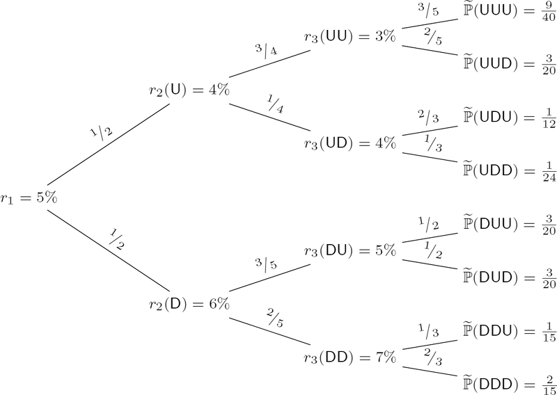
Consider a nonrecombining binomial tree model whose risk-neutral probabilities and interest rates are as shown in Figure 8.5. Compute the time-0 price of (i) a zero-coupon bond maturing at time 3 and (ii) a coupon bond with payments $C_1=C_2=C_3=\frac{1}{3}$.

Solution. First, we compute the time-0 prices Z0,n of zero-coupon bonds maturing at times n =1, 2, 3, respectively:

$\begin{array}{c}{Z}_{0,3}={\displaystyle \sum _{{\omega }_1,{\omega }_2,{\omega }_3\in \left\{\text{D},\text{U}\right\}}\frac{1}{\left(1+r_1\right)\left(1+r_2\left({\omega }_1\right)\right)\left(1+r_3\left({\omega }_1{\omega }_2\right)\right)}\tilde{\mathbb{P}}\left({\omega }_1{\omega }_2{\omega }_3\right)}\\ ={\displaystyle \sum _{{\omega }_{1,}{\omega }_2\in \left\{\text{D},\text{U}\right\}}\frac{1}{\left(1+r_1\right)\left(1+r_2\left({\omega }_1\right)\right)\left(1+r_3\left({\omega }_1{\omega }_2\right)\right)}\tilde{\mathbb{P}}\left(A_{{\omega }_1{\omega }_2}\right)}\\ =\frac{1/5}{1.05\cdot 1.06\cdot 1.07}+\frac{3/10}{1.05\cdot 1.06\cdot 1.05}+\frac{1/8}{1.05\cdot 1.04\cdot 1.04}+\frac{3/8}{1.05\cdot 1.04\cdot 1.03}\\ \cong 0.868116,\end{array}$

$\begin{array}{c}{Z}_{0,2}={\displaystyle \sum _{{\omega }_1,{\omega }_2\in \left\{\text{D},\text{U}\right\}}\frac{1}{\left(1+r_1\right)\left(1+r_2\left({\omega }_1\right)\right)}\tilde{\mathbb{P}}\left(A_{{\omega }_1{\omega }_2}\right)={\displaystyle \sum _{{\omega }_1\in \left\{\text{D},\text{U}\right\}}\frac{1}{\left(1+r_1\right)\left(1+r_2\left({\omega }_1\right)\right)}\tilde{\mathbb{P}}\left(A_{{\omega }_1}\right)}}\\ =\frac{1/2}{1.05\cdot 1.06}+\frac{1/2}{1.05\cdot 1.04}\cong 0.907112,\\ Z_{0,1}={\displaystyle \sum _{{\omega }_1\in \left\{\text{D},\text{U}\right\}}\frac{1}{1+r_1}\tilde{\mathbb{P}}\left(A_{{\omega }_1}\right)=\frac{1}{1+r_1}=\frac{1}{1.05}\cong \mathrm{0.952381.}}\end{array}$

In the above calculations, we used the risk-neutral probabilities $\tilde{\mathbb{P}}\left(A_{{\omega }_1{\omega }_2}\right)$ computed from transition probabilities, which are given as weights in Figure 8.5:

$\begin{array}{c}\tilde{\mathbb{P}}\left(A_{\text{DD}}\right)=\tilde{\mathbb{P}}\left(A_{\text{D}}\right)\tilde{\mathbb{P}}\left(A_{\text{DD}}|A_{\text{D}}\right)=\frac{1}{2}\cdot \frac{2}{5}=\frac{1}{5},\\ \tilde{\mathbb{P}}\left(A_{\text{DU}}\right)=\tilde{\mathbb{P}}\left(A_{\text{D}}\right)\tilde{\mathbb{P}}\left(A_{\text{DU}}|A_{\text{D}}\right)=\frac{1}{2}\cdot \frac{3}{5}=\frac{3}{10},\\ \tilde{\mathbb{P}}\left(A_{\text{UD}}\right)=\tilde{\mathbb{P}}\left(A_{\text{U}}\right)\tilde{\mathbb{P}}\left(A_{\text{UD}}|A_{\text{U}}\right)=\frac{1}{2}\cdot \frac{1}{4}=\frac{1}{8},\\ \tilde{\mathbb{P}}\left(A_{\text{UU}}\right)=\tilde{\mathbb{P}}\left(A_{\text{U}}\right)\tilde{\mathbb{P}}\left(A_{\text{UU}}|A_{\text{U}}\right)=\frac{1}{2}\cdot \frac{3}{4}=\frac{3}{8}.\end{array}$

So, the price of the zero-coupon bond maturing at time 3 is Z0,3 ≅ 0.868116. The price of the coupon bond is

$\frac{1}{3}\cdot Z_{0,1}+\frac{1}{3}\cdot Z_{0,2}+\frac{1}{3}\cdot Z_{0,2}=\frac{0.952381+0.907112+0.868116}{3}\cong \mathrm{0.909203.}$

In Example 8.8, the bond prices are calculated using the risk-neutral probabilities given us a priori. In practice, we deal with the reverse situation: the market prices of bonds with different term structures are known and then the risk-neutral probability measure $\tilde{\mathbb{P}}$ needs to be determined. Recall that the discounted bond price processes ${\left\{{\overline{Z}}_{n,m}=Z_{n,m}/B_n\right\}}_{0\le n\le m}$ are $\tilde{\mathbb{P}}$-martingales for all m = 1, 2,...,T. Therefore, the risk-neutral probabilities can be found by solving

$\{\begin{array}{l}\left(1+r_{n+1}\left({\omega }_1...{\omega }_n\right)\right)Z_{n,m}\left({\omega }_1...{\omega }_n\right)=Z_{n+1,m}\left({\omega }_1...{\omega }_n\text{D}\right)\tilde{\mathbb{P}}\left(A_{{\omega }_1...{\omega }_n\text{D}}|A_{{\omega }_1...{\omega }_n}\right)\hfill \\ +Z_{n+1,m}\left({\omega }_1...{\omega }_n\text{U}\right)\tilde{\mathbb{P}}\left(A_{{\omega }_1...{\omega }_n\text{U}}|A_{{\omega }_1...{\omega }_n}\right)\hfill \\ \tilde{\mathbb{P}}\left(A_{{\omega }_1...{\omega }_n\text{D}}|A_{{\omega }_1...{\omega }_n}\right)+\tilde{\mathbb{P}}\left(A_{{\omega }_1...{\omega }_n\text{U}}|A_{{\omega }_1...{\omega }_n}\right)=1\hfill \end{array}\text{ (8.32)}$

for all ω1,...,ωn ∊{D, U} and all n and m with 1 ≤ n + 1 <m ≤ T. Clearly, under the no-arbitrage assumption, all probabilities have to be between 0 and 1 and have to be independent of maturity.

For example, in the three-period case, we have three zero-coupon bonds with maturities m = 1, m = 2, and m = 3, respectively. The bond prices can be organized in a binomial tree, given in Figure 8.6. Since the face value of any ZCB is one, we omit the values Zm,m for all m = 1, 2, 3 in the above figure and truncate the tree to two periods. To find the state probabilities $\tilde{\mathbb{P}}\left(A_{\text{D}}\right)$ and $\tilde{\mathbb{P}}\left(A_{\text{U}}\right)$, we solve either

$Z_{0,2}=\frac{1}{1+r_1}\left[Z_{1,2}\left(\text{D}\right)\tilde{\mathbb{P}}\left(A_{\text{D}}\right)+Z_{1,2}\left(\text{U}\right)\tilde{\mathbb{P}}\left(A_{\text{U}}\right)\right]$

or

$Z_{0,3}=\frac{1}{1+r_1}\left[Z_{1,3}\left(\text{D}\right)\tilde{\mathbb{P}}\left(A_{\text{D}}\right)Z_{1,3}\left(\text{U}\right)\tilde{\mathbb{P}}\left(A_{\text{U}}\right)\right].$

The result has to be independent of maturity or there is an arbitrage opportunity otherwise. The proof of this fact is left as an exercise for the reader. To find the conditional probabilities $\tilde{\mathbb{P}}\left\{A_{{\omega }_1{\omega }_2}|A_{{\omega }_1}\right\}$ for ω1,ω2 ∊{D, U}, we solve the following equations:

$\begin{array}{c}{Z}_{1,3}\left(\text{D}\right)=\frac{1}{1+r_2\left(\text{D}\right)}\left[Z_{2,3}\left(\text{DD}\right)\tilde{\mathbb{P}}\left(A_{\text{DD}}|A_{\text{D}}\right)+Z_{2,3}\left(\text{DU}\right)\tilde{\mathbb{P}}\left(A_{\text{DU}}|A_{\text{D}}\right)\right]\\ Z_{1,3}\left(\text{U}\right)=\frac{1}{1+r_2\left(\text{U}\right)}\left[Z_{2,3}\left(\text{UD}\right)\tilde{\mathbb{P}}\left(A_{\text{UD}}|A_{\text{U}}\right)+Z_{2,3}\left(\text{UU}\right)\tilde{\mathbb{P}}\left(A_{\text{UU}}|A_{\text{U}}\right)\right].\end{array}$

Note that we also use the fact that $\tilde{\mathbb{P}}$ is a probability measure. Since the value of a ZCB at maturity is always one, the above process cannot be used to determine the probabilities $\tilde{\mathbb{P}}\left(A_{{\omega }_1{\omega }_2{\omega }_3}|A_{{\omega }_1{\omega }_2}\right)$ for the last period. However, these probabilities are not required for pricing bonds and other interest rate derivatives.

8.5 Exercises

1. Exercise 8.1. Prove that a multi-period model is complete iff every single-period sub-model is complete (Lemma 8.6).
2. Exercise 8.2. Consider a binomial model with stochastic volatility and stochastic interest rates presented in Section 8.4.1. Find a formula for the number of shares of stock, Δt, held at each time t ∊{0, 1, 2 ...,T − 1} by a self-financing portfolio strategy that replicates a derivative with a given payoff VT.

3. Exercise 8.3. Consider a two-period market model with four scenarios and two base assets: a risk-free asset B with the prices B0 = 50, B1 = 55, and B2 = 60 and a risky stock S whose prices are given by

   Scenario	S0(ω)	S1(ω)	S2(ω)
   ω1	50	60	70
   ω2	50	60	50
   ω3	50	45	50
   ω4	50	45	40

   1. (a) Find the EMM relative to the numéraire g = B.
   2. (b) If instead S2(ω1) = 65, show how to construct an arbitrage strategy.

4. Exercise 8.4. For the model described in Examples 8.3 and 8.4, construct a self-financing strategy replicating the payoff vector

   $V_2(\Omega )=\left[10,20,30,40,50,60,70,80,90\right].$

5. Exercise 8.5. Consider the two-period trinomial model with three base assets as given in Examples 8.3 and 8.4.

   1. (a) Construct the Radon–Nikodym process ${\left\{{\varrho }_t\right\}}_{t\in \left\{0,1,2\right\}}$ of ${\tilde{\mathbb{P}}}^{\left(S1\right)}$ w.r.t. ${\tilde{\mathbb{P}}}^{\left(B\right)}$.
   2. (b) Using the result of Example 8.5, find the EMM ${\tilde{\mathbb{P}}}^{\left(s^1\right)}$.
6. Exercise 8.6. Consider the following game. There is a set of 3 coins labelled 1, 2, and 3. The first coin has probability of heads 0.4, the second coin has probability of heads 0.6, and the third coin is fair. Your initial capital is $1. You toss the three coins in turn. If coin n results in heads, then your wealth is increased by factor of n + 1; otherwise, the wealth is decreased by factor of n + 1, where n = 1, 2, 3. Draw a scenario tree indicating possible outcomes along with their probabilities. Find the distribution of your final wealth.
7. Exercise 8.7. For a given integer m with 1 ≤ m ≤ T, consider a contract that pays rm at time m. Show that the time-zero no-arbitrage price of this contract is equal to Z0,m−1 − Z0,m.

8. Exercise 8.8. For a given integer m with 1 ≤ m ≤ T, an m-period interest rate swap is a contract that makes payments S1,S2,...,Sm at times 1, 2,...,m, respectively, where Sn = K − rn for n = 1, 2,...,m, and K is a fixed rate.

   1. (a) Show that the time-zero no-arbitrage value of the swap contract is equal to

      $K{\displaystyle \sum _{n=1}^m{Z}_{0,n}-\left(1-Z_{0,m}\right).}$

   2. (b) Find the time-zero no-arbitrage value of a three-period swap with K = 4% for the model of Example 8.8.

9. Exercise 8.9. For a given integer m with 1 ≤ m ≤ T, an m-period interest rate cap is a contract that makes payments C1,C2,...,Cm at times 1, 2,...,m, respectively, where Cn =(rn − K)+ for n = 1, 2,...,m, and K is a fixed rate. An m-period interest rate floor is a contract that makes payments F1,F2,...,Fm at times 1, 2,...,m, respectively, where Fn =(K − rn)+ for n = 1, 2,...,m, and K is a fixed rate.

   1. (a) Consider interest rate swap, cap, and floor with the same period m. Show that the sum of the initial no-arbitrage values of the swap and cap gives the initial no-arbitrage value of the floor:

      ${\text{Swap}}_m+{\text{Cap}}_m={\text{Floor}}_m.$

   2. (b) Find the initial no-arbitrage values of the three-period floor and cap with K = 4% for the model in Example 8.8.
10. Exercise 8.10. Consider a binomial tree model for interest rates. Let the risk-free interest rates and no-arbitrage prices of bonds with all possible maturities be given. Show that the lack of arbitrage implies that the risk-neutral probabilities defined by (8.32) are independent of maturity.