T

Taguchi methods – An approach to design of experiments developed by Genichi Taguchi that uses a quadratic loss function; also called robust design.

Dr. Genichi Taguchi developed a practical approach for designing quality into products and processes. His methodology recognized that quality should not be defined as simply within or not within specifications, so he created a simple quadratic loss function to measure quality. The two figures below contrast the typical 0-1 loss function used in quality with the Taguchi quadratic loss function.

Technicians apply Taguchi methods on the manufacturing floor to improve products and processes. The goal is to reduce the sensitivity of engineering designs to uncontrollable factors or noise by maximizing the signal to noise ratio. This moves design targets toward the middle of the design space so external variation affects the behavior of the design as little as possible. This approach permits large reductions in both part and assembly tolerances, which are major drivers of manufacturing cost.

See Analysis of Variance (ANOVA), Design of Experiments (DOE), functional build, lean sigma, robust, tolerance.

takt time – The customer demand rate expressed as a time and used to pace production.

According to a German-English dictionary (http://dict.leo.org), “takt” is the German word for “beat” or “musical time.” Several sources define takt as the baton that an orchestra conductor uses to regulate the beat for the orchestra. However, this is not correct. The German word for baton is “taktstock.”

The Japanese picked up the German word and use it to mean the beat time or heart beat of a factory. Lean production uses takt time to set the production rate to match the market demand rate. Takt time, therefore, is the desired time between completions of a product, synchronized to the customer demand rate and can be calculated as (available production time)/(forecasted demand rate).

Takt time, therefore, is set by the customer demand rate, and should be adjusted when the forecasted market demand rate changes. If takt time and the customer demand rate do not match, the firm (and the supply chain) will have either too little or too much inventory.

For example, a factory has a forecasted market demand of 100 units per day, and the factory operates for 10 hours per day. The target production rate should be the same as the market demand rate (100 units per day or 10 units per hour). The takt time for this factory should be (10 hours/day)/(100 units/day) = 0.1 hours per unit, or 6 minutes per unit. The factory should complete 1 unit about every 6 minutes, on average.

Many lean manufacturing consultants do not seem to understand the difference between a rate and a time and use the term “takt time” to mean the target production rate. However, a rate is measured in units per hour and a time is measured in hours (or minutes) per unit. For example, a production rate of 10 units per hour translates into a takt time of 6 minutes per unit.

Takt time is nearly identical to the traditional industrial engineering definition of cycle time, which is the target time between completions. The only difference between takt time and this type of cycle time is that takt time is defined by the market demand rate, whereas cycle time is not necessarily defined by the market demand.

Some people confuse takt time and throughput time. It is possible to have a throughput time of 6 weeks and have a takt time of 6 seconds. Takt time is the time between completions and can be thought of as time between units “falling off the end of the line.” The cycle time entry compares cycle time and throughput time.

See cycle time, heijunka, leadtime, lean thinking, pacemaker, pitch.

tally sheet – See checksheet.

tampering – The practice of adjusting a stable process and therefore increasing process variation.

Tampering is over-reacting to common cause variation and therefore always increasing variation.

See common cause variation, control chart, quality management, special cause variation, Statistical Process Control (SPC), Statistical Quality Control (SQC).

tardiness – See service level.

tare weight – (1) In a shipping/logistics context: The weight of an empty vehicle before the products are loaded; also called unladen weight. (2) In a packaging context: The weight of an empty shipping container or package.

The weight of the goods carried (the net weight) can be determined by subtracting the tare weight from the total weight, which is called the gross weight or laden weight. The tare weight can be useful for estimating the cost of goods carried for taxation and tariff purposes. This is a common practice for tolls related to barge, rail, and road traffic, where the toll varies with the value of the goods. Tare weight is often printed on the sides of railway cars and transport vehicles.

See gross weight, logistics, net weight, scale count, tariff.

target cost – The desired final cost for a new product development effort.

Many firms design a product, estimate the actual cost, and then add the margin to set the price. In contrast to this practice, with a target costing strategy, the firm determines the price based on the market strategy and then determines the target cost by subtracting the desired margin. The resulting “target cost” becomes the requirement for the product design team. The four major steps of target costing are:

1. Determine the price – The amount customers are willing to pay for a product or service with specified features and functions.

2. Set the target cost per unit and in total – The target cost per unit is the market price less the required margin. The total target cost is the per unit target cost multiplied by the expected number of units sold over its life.

3. Compare the total target cost to the currently feasible total cost to create the cost reduction target – The currently feasible total cost is the cost to make the product, given current design and process capabilities. The difference between the total target cost and currently feasible cost is the cost reduction target.

4. Design (or redesign) products and processes to achieve the cost reduction target – This can be an iterative process until both the product or service and its cost meet marketing and financial objectives.

See job order costing, target price.

target market – The group of customers that a business intends to serve.

See market share, strategy map.

target inventory – See order-up-to level.

target price – The practice of setting a sales price based on what the market will bear rather than on a standard cost.

The target price is the price at which the firm believes a seller will buy a product based on market research. The easiest approach for determining a target price is to study similar products sold by competitors. The target price may be used to calculate the target cost. In an investment context, the target price is the price at which a stockholder is willing to sell his or her stock.

See Customer Relationship Management (CRM), target cost.

tariff – A tax on import or export trade.

An ad valorem tariff is set as a percentage of the value. A specific tariff is not based on the value.

See facility location, General Agreement on Tariffs and Trade (GATT), tare weight, trade barrier.

task interleaving – A warehouse management term for combining tasks, such as picking, put away, and cycle counting, on a single trip to reduce deadheading (driving empty) for materials handling equipment.

The main idea of task interleaving is to reduce deadheading for materials handling equipment, such as forklift trucks in a warehouse or distribution center. Task interleaving is often used with put away, picking, and cycle counting tasks. For example, a stock picker might put away a pallet and then pick another pallet and move it to the loading dock. Although task interleaving is used primarily in pallet operations, it can be used with any type of materials handling equipment. Benefits of task interleaving include reduced travel time, increased productivity, less wear on lift trucks, reduced energy usage, and better on-time delivery.

Gilmore (2005) suggests that a Warehouse Management System (WMS) task interleaving system must consider permission, proximity, priority, and the age of the task (time). He also recommends that firms initially implement a WMS system without interleaving so personnel can learn the basics before trying interleaving.

See picking, slotting, warehouse, Warehouse Management System (WMS).

technological forecasting – The process of predicting the future characteristics and timing of technology.

The prediction usually estimates the future capabilities of a technology. The two major methods for technological forecasting include time series and judgmental methods. Time series forecasting methods for technological forecasting fit a mathematical model to historical data to extrapolate some variable of interest into the future. For example, the number of millions of instructions per second (MIPS) for a computer is fairly predictable using time series methods. (However, the underlying technology to achieve that performance will change at discrete points in time.) Judgmental forecasting may also be based on projections of the past, but information sources in such models rely on the subjective judgments of experts.

The growth pattern of a technological capability is similar to the growth of biological life. Technologies go through an invention phase, an introduction and innovation phase, a diffusion and growth phase, and a maturity phase. This is similar to the S-shaped growth of biological life. Technological forecasting helps estimate the timing of these phases. This growth curve forecasting method is particularly useful in determining the upper limit of performance for a specific technology.

See Delphi forecasting, forecasting, technology road map.

technology push – A business strategy that develops a high-tech/innovative product with the hope that the market will embrace it; in contrast, a market pull strategy develops a product in response to a market need.

See operations strategy.

technology road map – A technique used by many businesses and research organizations to plan the future of a particular process or product technology.

The goal of a technology roadmap is to anticipate externally driven technological innovations by mapping them on a timeline. The technology roadmap can then be linked with the research, product development, marketing, and sourcing. Some of the benefits of technology roadmapping include:

• Support the organization’s strategic planning processes with respect to new technologies.

• Plan for the integration of new technologies into current products.

• Identify business opportunities for leveraging new technologies in new products.

• Identify needs for technical knowledge.

• Inform sourcing decisions, resource allocation, and risk management decisions.

One approach for structuring the technology roadmapping process is to use a large matrix on a wall to capture the ideas. The top row should be labeled Past → Now → Plans → Future → Vision. The left column has the rows labeled markets, products, technologies, and resources.

• The markets row is used to explore markets, customers, competitors, environment, industry, business trends, threats, objectives, milestones, and strategies.

• The products row is used to explore products, services, applications, performance capabilities, features, components, families, processes, systems, platforms, opportunities, requirements, and risks.

• The technologies row is used to map new technologies, competencies, and knowledge.

• The resources row is used for skills, partnerships, suppliers, facilities, infrastructure, science, and R&D projects.

Post-it Notes are then used to “map” and link each of these dimensions over time.

The Centre for Technology Management at the University of Cambridge has a number of publications on this topic at www.ifm.eng.cam.ac.uk/ctm/publications/tplan. Their standard “T-Plan” process includes four major steps that focus on (1) the market (performance dimensions, business drivers, SWOT, gaps), (2) the product (features, strategy, gaps), (3) technology (solutions, gaps), and (4) roadmapping (linking technology resources to future market requirements). Technology roadmapping software is offered by www.roadmappingtechnology.com. The University of Minnesota Technological Leadership Institute (TLI) (http://tli.umn.edu) makes technology roadmapping a key topic in many of its programs.

See disruptive technology, New Product Development (NPD), product life cycle management, technological forecasting.

technology transfer – The process of sharing skills, expertise, knowledge, processes, technologies, scientific research, and intellectual property across different organizations, such as research laboratories, governments, universities, joint ventures, or subsidiaries.

Technology transfer can occur in three ways: (1) giving it away through technical journals, conferences, or free training and technical assistance, (2) commercial transactions, such as licensing patent rights, marketing agreements, co-development activities, exchange of personnel, and joint ventures, and (3) theft through industrial espionage or reverse engineering.

See intellectual property (IP), knowledge management, reverse engineering.

telematics – The science of sending, receiving, and storing information via telecommunication devices.

According to Wikipedia, the word “telematics” is now widely associated with the use of Global Positioning System (GPS) technology integrated with computers and mobile communications technology in automotive and trucking navigation systems. This technology is growing in importance in the transportation industry. Some important applications of telematics include the following:

• In-car infotainment

• Navigation and location

• Intelligent vehicle safety

• Fleet management

• Asset monitoring

• Risk management

See Global Positioning System (GPS), logistics.

termination date – A calendar date by which a product will no longer be sold or supported.

Many manufacturing and distribution companies use a policy of having a “termination date” for products and components. A product (and its associated unique components) is no longer sold or supported after the termination date. The advantages of having a clearly defined termination date policy include:

• Provides a clear plan for every functional area in the organization that deals with products (manufacturing, purchasing, inventory, service, engineering, and marketing). This facilitates an orderly, coordinated phaseout of the item.

• Communicates to the salesforce and the market that the product will no longer be supported (or at least no longer be sold) after the termination date. This often provides incentive for customers to upgrade.

• Allows manufacturing and inventory planners to bring down the inventories for all unique components needed for the product in a coordinated way.

Best practices for a termination date policy include the following policies: (1) plan ahead many years to warn all stakeholders (this includes marketing, sales, product management, purchasing, and manufacturing), (2) ensure that all functions (and divisions) have “buy-in” to the termination date, and (3) do not surprise customers by terminating a product without proper notice.

See all-time demand, obsolete inventory, product life cycle management.

terms – A statement of a seller’s payment requirements.

Payment terms generally include discounts for prompt payment, if any, and the maximum time allowed for payment. The shipping terms determine who is responsible for the freight throughout the shipment. Therefore, a shipper will only be concerned about tracking the container to the point where another party takes ownership. This causes problems with container tracking because information may not be shared throughout all links in the supply chain.

See Accounts Payable (A/P), Cash on Delivery (COD), demurrage, FOB, Incoterms, invoice, waybill.

theoretical capacity – See capacity.

Theory of Constraints (TOC) – A management philosophy developed by Dr. Eliyahu M. Goldratt that focuses on the bottleneck resources to improve overall system performance.

The Theory of Constraints (TOC) recognizes that an organization usually has just one resource that defines its capacity. Goldratt (1992) argues that all systems are constrained by one and only one resource. As Goldratt states, “A chain is only as strong as its weakest link.” This is an application of Pareto’s Law to process management and process improvement. TOC concepts are consistent with managerial economics that teach that the setup cost for a bottleneck resource is the opportunity cost of the lost gross margin and that the opportunity cost for a non-bottleneck resource is nearly zero.

The “constraint” is the bottleneck, which is any resource that has capacity less than the market demand. Alternatively, the constraint can be defined as the process that has the lowest average processing rate for producing end products. The constraint (the bottleneck) is normally defined in terms of a resource, such as a machine, process, or person. However, the TOC definition of a constraint can also include tools, people, facilities, policies, culture, beliefs, and strategies. For example, this author observed that the binding constraint in a business school in Moscow in 1989 was the mindset of the dean (rector) who could not think beyond the limits of Soviet Communism, even for small issues, such as making photocopies⁵⁸.

The Goal (Goldratt 1992) and the movie of the same name, include a character named Herbie who slowed down a troop of Boy Scouts as they hiked though the woods. Herbie is the “bottleneck” whose pace slowed down the troop. The teaching points of the story for the Boy Scouts are (1) they needed to understand that Herbie paced the operation (i.e., the troop could walk no faster than Herbie) and (2) they needed to help Herbie with his load (i.e., the other Scouts took some of Herbie’s bedding and food so Herbie could walk faster). In the end, the troop finished the hike on-time because it had better managed Herbie, the bottleneck.

According to TOC, the overall performance of a system can be improved when an organization identifies its constraint (the bottleneck) and manages the bottleneck effectively. TOC promotes the following five-step methodology:

1. Identify the system constraint – No improvement is possible unless the constraint or weakest link is found. The constraint can often be discovered by finding the largest queue.

2. Exploit the system constraints – Protect the constraint (the bottleneck) so no capacity is wasted. Capacity can be wasted by (1) starving (running out of work to process), (2) blocking (running out of an authorized place to put completed work), (3) performing setups, or (4) working on defective or low-priority parts. Therefore, it is important to allow the bottleneck to pace the production process, not allow the bottleneck to be starved or blocked, focus setup reduction efforts on the bottleneck, increase lotsizes for the bottleneck, and inspect products before the constraint so no bottleneck time is wasted on defective parts.

3. Subordinate everything else to the system constraint – Ensure that all other resources (the unconstrained resources) support the system constraint, even if this reduces the efficiency of these resources. For example, the other processes can produce smaller lotsizes so the constrained resource is never starved. The unconstrained resources should never be allowed to overproduce.

4. Elevate the system constraints – If this resource is still a constraint, find more capacity. More capacity can be found by working additional hours, using alternate routings, purchasing capital equipment, or subcontracting.

5. Go back to Step 1 – After this constraint problem is solved, go back to the beginning and start over. This is a continuous process of improvement.

Underlying Goldratt’s work is the notion of synchronous manufacturing, which refers to the entire production process working in harmony to achieve the goals of the firm. When manufacturing is synchronized, its emphasis is on total system performance, not on localized measures, such as labor or machine utilization.

The three primary TOC metrics are throughput (T), inventory (I), and operating expenses (OE), often called T, I, and OE. Throughput is defined as sales revenue minus direct materials per time period. Inventory is defined as direct materials at materials cost. Operating expenses include both labor and overhead. Bottleneck management will result in increased throughput, reduced inventory, and the same or better operating expense.

See absorption costing, bill of resources, blocking, bottleneck, buffer management, CONWIP, critical chain, current reality tree, Drum-Buffer-Rope (DBR), facility layout, future reality tree, gold parts, Herbie, Inventory Dollar Days (IDD), lean thinking, opportunity cost, overhead, pacemaker, Pareto’s Law, process improvement program, routing, setup cost, setup time reduction methods, starving, synchronous manufacturing, throughput accounting, Throughput Dollar Days (TDD), transfer batch, utilization, variable costing, VAT analysis.

Theta Model – A forecasting model developed by Assimakopoulos and Nikolopoulos (2000) that combines a longterm and short-term forecast to create a new forecast; sometimes called the Theta Method.

The M3 Competition runs a “race” every few years to compare time series forecasting methods on hundreds of actual times series (Ord, Hibon, & Makridakis 2000). The winner of the 2000 competition was a relatively new forecasting method called the “Theta Model” developed by Assimakopoulos and Nikolopoulos (2000). This model was difficult to understand until Hyndman and Billah (2001) simplified the mathematics. More recently, Assimakopoulos and Nikolopoulos (2005) wrote their own simplified version of the model. Although the two simplified versions are very similar in intent, they are not mathematically equivalent.

Theta Model forecasts are the average (or some other combination) of a longer-term and a shorter-term forecast. The longer-term forecast can be a linear regression fit to the historical demand, and the shorter-term forecast can be a forecast using simple exponential smoothing. The Theta Model assumes that all seasonality has already been removed from the data using methods, such as the centered moving average. The apparent success of this simple time series forecasting method is that the exponential smoothing component captures the “random walk” part of the time series, and the least squares regression trend line captures the longer-term trend.

See exponential smoothing, forecasting, linear regression.

Thiel’s U – An early Relative Absolute Error (RAE) measure of forecast errors developed by Henri Thiel (1966).

Thiel’s U statistic (or Thiel’s inequality coefficient) is a metric that compares forecasts to an upper bound on the naïve forecast from a random walk, which uses the actual value from the previous period as the forecast for this period (Thiel 1966). Thiel proposed two measures for forecast error that Armstrong calls U₁ and U₂. SAP uses still another variant of Thiel’s coefficient, labeled U₃ below.

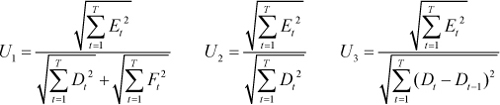
According to Armstrong and Collopy (1992), the U₂ metric has better statistical properties than U₁ or U₃. Although Thiel’s U metrics are included in many forecasting tools and texts, Armstrong and Collopy do not recommend them because other RAE metrics are easier to understand and have better statistical properties.

See forecast error metrics, Mean Absolute Percent Error (MAPE), Relative Absolute Error (RAE).

Third Party Logistics (3PL) provider – A firm that provides outsourced services, such as transportation, logistics, warehousing, distribution, and consolidation to customers but does not take ownership of the product.

Third Party Logistics providers (3PLs) are becoming more popular as companies seek to improve their customer service capabilities without making significant investments in logistics assets, networks, and warehouses. The 3PL may conduct these functions in the client’s facility using the client’s equipment or may use its own facilities and equipment. The parties in a supply chain relationship include the following:

• First party – The supplier

• Second party – The customer

• Third party (3PL) – A company that offers multiple logistics services to customers, such as transportation, distribution, inbound freight, outbound freight, freight forwarding, warehousing, storage, receiving, cross-docking, customs, order fulfillment, inventory management, and packaging. In the U.S., the legal definition of a 3PL in HR4040 is “a person who solely receives, holds, or otherwise transports a consumer product in the ordinary course of business but who does not take title to the product” (source: www.scdigest.com, 2009).

• Fourth party (4PL) – An organization that manages the resources, capabilities, and technologies of multiple service providers (such as 3PLs) to deliver a comprehensive supply chain solution to its clients.

With a 3PL, the supplier firm outsources its logistics to two or more specialist firms (3PLs) and then hires another firm (the 4PL) to coordinate the activities of the 3PLs. 4PLs differ from 3PLs in the following ways (source: www.scdigest.com, January 1, 2009):

• The 4PL organization is often a separate entity established as a joint venture or long-term contract between a primary client and one or more partners.

• The 4PL organization acts as a single interface between the client and multiple logistics service providers.

• All aspects of the client’s supply chain are managed by the 4PL organization.

• It is possible for a 3PL to form a 4PL organization within its existing structure.

See the International Warehouse Logistics Association (www.iwla.com) site for more information.

See bullwhip effect, consolidation, customer service, fulfillment, joint venture, logistics, receiving, warehouse.

throughput accounting – Accounting principles based on the Theory of Constraints developed by Goldratt.

Throughput is the rate at which an organization generates money through sales. Goldratt defines throughput as the difference between sales revenue and unit-level variable costs, such as materials and power. Cost is the most important driver for our operations decisions, yet costs are unreliable due to the arbitrary allocation of overhead, even with Activity Based Costing (ABC). Because the goal of the firm is to make money, operations can contribute to this goal by managing three variables:

• Throughput (T) = Revenue less materials cost less out-of-pocket selling costs (Note that this is a rate and is not the same as the throughput time.)

• Inventory (I) = Direct materials cost and other truly variable costs with no overhead

• Operating expenses (OE) = Overhead and labor cost (the things that turn the “I” into “T”)

Throughput accounting is a form of contribution accounting, where all labor and overhead costs are ignored. The only cost that is considered is the direct materials cost. Throughput accounting is applied to the bottleneck (the constraint) using the following key performance measurements: output, setup time (average setup time by product and total setup time per period), downtime (planned and emergency), and yield rate. The bottleneck has the greatest impact on the throughput accounting measures (T, I, and OE), which in turn affect the goal of making money for the firm. Noreen, Smith, and Mackey (1995) is a good reference on this subject.

See absorption costing, Activity Based Costing (ABC), focused factory, Inventory Dollar Days (IDD), overhead, Theory of Constraints (TOC), Throughput Dollar Days (TDD), variable costing, Work-in-Process (WIP) inventory.

Throughput Dollar Days (TDD) – A Theory of Constraints (TOC) measure of the reliability of a supply chain defined in terms of the dollar days of late orders.

The entry Inventory Dollar Days (IDD) has much more detail on this measure.

See Inventory Dollar Days (IDD), operations performance metrics, Theory of Constraints (TOC), throughput accounting.

throughput ratio – See value added ratio.

throughput time – See cycle time.

tier 1 supplier – A sourcing term for an immediate supplier; a tier 2 supplier is a supplier to a supplier.

See purchasing, supply chain management.

time bucket – A time period used in planning and forecasting systems.

The time bucket (period) for most MRP systems is a day. These systems are often called bucketless because they use date-quantity detail rather than weekly or monthly time buckets. In contrast, many forecasting systems forecast in monthly or weekly time buckets.

See Croston’s Method, exponential smoothing, finite scheduling, forecasting, Materials Requirements Planning (MRP), production planning.

time burglar – A personal time management term that refers to anything (including a person) that steals time from someone else; someone who wastes the time of another person.

Time burglars are people who often stop by and ask, “Got a minute?” and then proceed to launch into 20 minutes of low-value discussion. Some situations, such as a friend stopping by to say “hello,” are just minor misdemeanors, but disruptions that arrive during a critical work situation could be considered a crime.

The key time management principle for managers is to explain the situation and then offer to schedule another time for a visit. A reasonable script is, “I can see this is going to take some more time to discuss. Let’s schedule some time to talk about this further. When is a good time for you?”

The term “time burglar” can also be applied to junk e-mail, unnecessary meetings, too much TV, surring the Internet, and other time wasting activities. Time burglars are everywhere, so stop them before they strike.

See personal operations management.

time fence – A manufacturing planning term used for a time period during which the Master Production Schedule (MPS) cannot be changed; sometimes called a planning time fence.

The time fence is usually defined by a planning period in days (e.g., 21 days) during which the Master Production Schedule (MPS) cannot be altered and is said to be frozen. The time fence separates the MPS into a firm order period followed by a tentative time period. The purpose of a time fence policy is to reduce shortterm schedule disruptions for both manufacturing and suppliers and improve on-time delivery for customers by stabilizing the MPS and reducing “system nervousness.”

Oracle makes a distinction between planning, demand, and release time fences. More on this topic can be found at http://download.oracle.com/docs/cd/A60725_05/html/comnls/us/mrp/tfover.htm (January 11, 2011).

See cumulative leadtime, firm planned order, Master Production Schedule (MPS), Materials Requirements Planning (MRP), planned order, planning horizon, premium freight, Sales & Operations Planning (S&OP).

time in system – The total start to finish time for a customer or customer order; also called customer leadtime.

The time in system is the turnaround time for a customer or customer order. In the queuing context, time in system is the sum of the wait time (the time in queue before service begins) and the service time.

Do not confuse the actual time in system for a single customer, the average time in system across a number of customers, and the planned time in system parameter, which is used for planning purposes.

See customer leadtime, cycle time, leadtime, Little’s Law, queuing theory, turnaround time, wait time.

time management – See personal operations management.

time study – A work measurement practice of collecting data on work time by observation, typically using a stop watch or some other timing device.

The average actual time for a worker in the time study is adjusted by his or her performance rating to determine the normal time for a task. The standard time is then the normal time with an allowance for breaks.

See normal time, performance rating, scientific management, standard time, work measurement, work sampling.

time to market – The time it takes to develop a new product from an initial idea (the product concept) to initial market sales; sometimes called speed to market.

In many industries, a short time to market can provide a competitive advantage, because the firm “first to market” with a new product can command a higher margin, capture a larger market share, and establish its brand as the strongest brand in the market. Precise definitions of the starting and ending points vary from one firm to another, and may even vary between products within a single firm. The time to market includes both product design and commercialization. Time to volume is a closely related concept.

See clockspeed, market share, New Product Development (NPD), product life cycle management, time to volume, time-based competition.

time to volume – The time from the start of production to the start of large-scale production.

See New Product Development (NPD), time to market.

time-based competition – A business strategy to (a) shorten time to market for new product development, (b) shorten manufacturing cycle times to improve quality and reduce cost, and (c) shorten customer leadtimes to stimulate demand.

Stalk (1988) and Stalk and Hout (1990) make strong claims about the profitability of a time-based strategy. The strategy map entry presents a causal map that summarizes and extends this competition strategy. The benefits of a time-based competition strategy include: (1) segmenting the demand to target the time-sensitive and price-insensitive customers and increase margins, (2) reducing work-in-process and finished goods inventory, (3) driving out non-value activities (e.g., JIT and lean manufacturing concepts), and (4) bringing products to market faster. These concepts are consistent with the Theory of Constraints and lean thinking.

See agile manufacturing, flow, operations strategy, Quick Response Manufacturing, resilience, time to market, value added ratio.

Time Phased Order Point (TPOP) – An extension of the reorder point system that uses the planned future demand to estimate the date when the inventory position will hit the safety stock level; it then backschedules using the planned leadtime from that date to determine a start date for a planned order.

The Time Phased Order Point (TPOP) system is used to determine the order timing in all Materials Requirements Planning (MRP) systems. TPOP uses the gross requirements (the planned demand) to determine the date when the planned inventory position will hit the safety stock level. It then uses the planned leadtime to plan backward in time (backschedule) to determine the start date for the next planned order. The lotsize (order quantity) can be determined with any lotsizing rule, such as lot-for-lot, fixed order quantity, EOQ, day’s supply, week’s supply, etc. TPOP can be used over the planning horizon to create many planned orders.

See lotsizing methods, Materials Requirements Planning (MRP), reorder point, safety stock.

time series forecasting – A forecasting method that identifies patterns in historical data to make forecasts for the future; also called intrinsic forecasting.

A time series is a set of historical values listed in time order (such as a sales history). A time series can be broken (decomposed) into a level (or mean), trend, and seasonal patterns. If the level, trend, and seasonal patterns are removed from a time series, all that remains is what appears to be random error (white noise). Box-Jenkins methods attempt to identify and model the autocorrelation (serial correlation) structure in this error.

A moving average is the simplest time series forecast method, but it is not very accurate because it does not include either trend or seasonal patterns. The Box-Jenkins method is the most sophisticated, but is more complicated than most managers can handle. The exponential smoothing model with trend and seasonal factors is a good compromise for most firms.

Univariate time series methods simply extrapolate a single time series into the future. Multivariate time series methods consider historical data for several related variables to make forecasts.

See autocorrelation, Box-Jenkins forecasting, Croston’s Method, Durbin-Watson statistic, exponential smoothing, forecasting, linear regression, moving average, seasonality, trend.

time-varying demand lotsizing problem – The problem of finding the set of lotsizes that will “cover” the demand over the time horizon and will minimize the sum of the ordering and carrying costs.

Common approaches for solving this problem include the Wagner-Whitin lotsizing algorithm, the Period Order Quantity (POQ), the Least Total Cost method, the Least Unit Cost method, and the Economic Order Quantity. Only the Wagner-Whitin algorithm is guaranteed to find the optimal solution. All other lotsizing methods are heuristics; however, the cost penalty in using these heuristics is generally small.

See Economic Order Quantity (EOQ), lotsizing methods, Period Order Quantity (POQ), Wagner-Whitin lotsizing algorithm.

TOC – See Theory of Constraints.

tolerance – An allowable variation from a predefined standard; also called specification limits.

All processes have some randomness, which means that no manufacturing process will ever produce parts that exactly achieve the “nominal” (target) value. Therefore, design engineers define tolerance (or specification) limits that account for this “common cause variation.” A variation from the standard is not considered significant unless it exceeds the upper or lower tolerance (specification) limit. Taguchi takes a different approach to this issue and creates a loss function around the nominal value rather than setting limits.

See common cause variation, Lot Tolerance Percent Defective (LTPD), process capability and performance, Taguchi methods.

ton-mile – A measure of freight traffic equal to moving one ton of freight one mile. See logistics.

tooling – The support devices required to operate a machine.

Tooling usually includes jigs, fixtures, cutting tools, molds, and gauges. In some manufacturing contexts, the requirements for specialized tools are specified in the bill of materials. Tooling is often stored in a tool crib.

See fixture, Gauge R&R, jig, manufacturing processes, mold.

total cost of ownership – The total cost that a customer incurs from before the purchase until the final and complete disposal of the product; also known as life cycle cost.

Some of these costs include search costs, purchase (acquisition) cost, purchasing administration, shipping (delivery), expediting, premium freight, transaction cost, inspection, rework, scrap, switching cost, installation cost, training cost, government license fees, royalty fees, Maintenance Repair Operations (service contracts, parts, labor, consumables, repair), information systems costs (support products, upgrades), inventory carrying cost, inventory redistribution/redeployment cost (moving inventory to a new location), insurance, end of life disposal cost, and opportunity costs (downtime, lost productive time, lost sales, lost profits, brand damage)⁵⁹.

Life cycle cost is very similar to the total cost of ownership. The only difference is that life cycle cost identifies cost drivers based on the stage in the product life cycle (introduction, growth, maturity, and decline). Both total cost of ownership and life cycle cost can have an even broader scope that includes research and development, design, marketing, production, and logistics costs.

See financial performance metrics, purchasing, search cost, switching cost, transaction cost.

Total Productive Maintenance (TPM) – A systematic approach to ensure uninterrupted and efficient use of equipment; also called Total Productive Manufacturing.

Total Productive Maintenance (TPM) is a manufacturing-led collaboration between operations and maintenance that combines preventive maintenance concepts with the kaizen philosophy of continuous improvement. With TPM, maintenance takes on its proper meaning to “maintain” rather than just repair. TPM, therefore, focuses on preventive and predictive maintenance rather than only on emergency maintenance. Some leading practices related to TPM include:

• Implement a 5S program with a standardized work philosophy.

• Apply predictive maintenance tools where appropriate.

• Use an information system to create work orders for regularly scheduled preventive maintenance.

• Use an information system to maintain a repair history for each piece of equipment.

• Apply autonomous maintenance, which is the concept of using operators to inspect and clean equipment without heavy reliance on mechanics, engineers, or maintenance people. (This is in contrast to the old thinking which required operators to wait for mechanics to maintain and fix their machines.)

• Clearly define cross-functional duties.

• Train operators to handle equipment related issues.

• Measure performance with Overall Equipment Effectiveness (OEE).

Some indications that a TPM program might be needed include frequent emergency maintenance events, long downtimes, high repair costs, reduced machine speeds, high defects and rework, long changeovers, high startup losses, high Mean Time to Repair (MTTR), and low Mean Time Between Failure (MTBF). Some of the benefits for a well-run TPM program include reduced cycle time, improved operational efficiency, improved OEE, improved quality, and reduced maintenance cost.

See 5S, autonomous maintenance, bathtub curve, downtime, maintenance, Maintenance-Repair-Operations (MRO), Manufacturing Execution System (MES), Mean Time Between Failure (MTBF), Mean Time to Repair (MTTR), Overall Equipment Effectiveness (OEE), reliability, reliability engineering, Reliability-Centered Maintenance (RCM), standardized work, Weibull distribution, work order.

Total Productive Manufacturing (TPM) – See Total Productive Maintenance (TPM).

Total Quality Management (TQM) – An approach for improving quality that involves all areas of the organization, including sales, engineering, manufacturing, and purchasing, with a focus on employee participation and customer satisfaction.

Total Quality Management (TQM) can involve a wide variety of quality control and improvement tools. TQM pioneers, such as Juran (1986), Deming (1986, 2000), and Crosby (1979) emphasized a combination of managerial principles and statistical tools. This term has been largely supplanted by lean sigma and lean programs and few practitioners or academics use this term today. The quality management, lean sigma, and lean entries provide much more information on this subject.

See causal map, defect, Deming’s 14 points, inspection, lean sigma, Malcolm Baldrige National Quality Award (MBNQA), PDCA (Plan-Do-Check-Act), quality management, quality trilogy, stakeholder analysis, Statistical Process Control (SPC), Statistical Quality Control (SQC), zero defects.

touch time – The direct value-added processing time.

See cycle time, run time, value added ratio.

Toyota Production System (TPS) – An approach to manufacturing developed by Eiji Toyoda and Taiichi Ohno at Toyota Motor Company in Japan; some people use TPS synonymously with lean thinking⁶⁰.

See autonomation, jidoka, Just-in-Time (TPS), lean thinking, muda.

T-plant – See VAT analysis.

TPM – See Total Productive Maintenance (TPM).

TPOP – See Time Phased Order Point (TPOP).

TPS – See Toyota Production System (TPS).

TQM – See Total Quality Management (TQM).

traceability – The capability to track items (or batches of items) through a supply chain; also known as lot traceability, serial number traceability, lot tracking, and chain of custody.

Lot traceability is the ability to track lots (batches of items) forward from raw materials through manufacturing and ultimately to end customers and also backward from end consumers back to the raw materials. Lot traceability is particularly important for food safety in food supply chains.

Serial number traceability is individual “serialized” items and is important in medical device supply chains. Petroff and Hill (1991) provide suggestions for designing lot and serial number traceability systems.

See Electronic Product Code (EPC), part number, supply chain management.

tracking signal – An exception report given when the forecast error is consistently positive or negative over time (i.e., the forecast error is biased).

The exception report signals the manager or analyst to intervene in the forecasting process. The intervention might involve manually changing the forecast, the trend, underlying average, and seasonal factors, or changing the parameters for the forecasting model. The intervention also might require canceling orders and managing both customer and supplier expectations.

Tracking signal measurement – The tracking signal is measured as the forecast bias divided by a measure of the average size of the forecast error.

Measures of forecast bias – The simplest measure of the forecast bias is to accumulate the forecast error over time (the cumulative sum) with the recursive equation R_t = R_t−1 + E_t, where R_t is the running sum of the errors and E_t is the forecast error in period t. The running sum of the errors is a measure of the bias and an exception report is generated when R_t gets “large.” Another variant is to use the smoothed average error instead of the running sum of the error. The smoothed error is defined as SE_t = (1 − α)SE_t−1 + αE_t.

Measures of the average size of the forecast error – One measure of the size of the average forecast error is the Mean Absolute Deviation (MAD). The MAD is defined as , where T is the number of periods of history. A more computationally efficient approach to measure the MAD is with the smoothed mean absolute error, which is defined as SMAD_t = (1 − α)SMAD_t−1 + α|E_t|, where alpha (α) is the smoothing constant (0 < α < 1). Still another approach is to replace the smoothed mean absolute deviation (SMAD_t) with the square root of the smoothed mean squared error, where the smoothed mean squared error is defined as SMSE_t = (1 − α)SMSE_t + αE_t². In other words, the average size of the forecast error can be measured as . The smoothed MAD is the most practical approach for most firms.

In summary, a tracking signal is a measure of the forecast bias relative to the average size of the forecast error and is defined by TS = bias/size. Forecast bias can be measured as the running sum of the error (R_t) or the smoothed error (SE_t); the size of the forecast error can be measured with the MAD, the smoothed mean absolute error (SMAD_t), or the square root of the mean squared error (SMAD_t). It is not clear which method is best.

See cumulative sum control chart, demand filter, exponential smoothing, forecast bias, forecast error metrics, forecasting, Mean Absolute Deviation (MAD), Mean Absolute Percent Error (MAPE), mean squared error (MSE).

trade barrier – Any governmental regulation or policy, such as a tariff or quota that restricts imports or exports.

See tariff.

trade promotion allowance – A discount given to retailers and distributors by a manufacturer to promote products; retailers and distributors sponsor advertising and other promotional activities or pass the discount along to consumers to encourage sales; also known as trade allowance, cooperative advertising allowance, advertising allowance, and ad allowance.

Trade promotions include slotting allowances, performance allowances, case allowances, and account specific promotions. Promotions can include newspaper advertisements, television and radio programs, in-store sampling programs, and slotting fees. Trade promotions are common in the consumer packaged goods (CPG) industry.

See consumer packaged goods, slotting.

traffic management – See Transportation Management System (TMS).

trailer – A vehicle pulled by another vehicle (typically a truck or tractor) used to transport goods on roads and highways; also called semitrailer, tractor trailer, rig, reefer, flatbed; in England, called articulated lorry.

Trailers are usually enclosed vehicles with a standard length of 45, 48, or 53 feet, internal width of 98 to 99 inches, and internal height of 105 to 110 inches. Refrigerated trailers are known as reefers and have an internal width of 90 to 96 inches and height of 96 to 100 inches. Semi-trailers usually have three axles, with the front axle having two wheels and the back two axles each having a pair of wheels for a total of 10 wheels.

See Advanced Shipping Notification (ASN), cube utilization, dock, intermodal shipments, less than truck load (LTL), logistics, shipping container, Transportation Management System (TMS).

transaction cost – The cost of processing one transaction, such as a purchase order.

In a supply chain management context, this is the cost of processing one purchase order.

See search cost, switching cost, total cost of ownership.

transactional process improvement – Improving repetitive non-manufacturing activities.

The term “transactional process improvement” is used by many lean sigma consultants to describe efforts to improve non-manufacturing processes in manufacturing firms and also improve processes in service organizations. Examples include back-office operations (e.g., accounting, human resources) and front-office operations (order-entry, customer registration, teller services).

The entities that flow through these processes may be information on customers, patients, lab specimens, etc. and may be stored on paper or in electronic form. The information often has to travel across several departments. Lean sigma programs can often improve transactional processes by reducing non-value-added steps, queue time, cycle time, travel time, defects, and cost while improving customer satisfaction.

See lean sigma, lean thinking, service management, waterfall scheduling.

transfer batch – A set of parts that is moved in quantities less than the production batch size.

When a batch of parts is started on a machine, smaller batches can be moved (transferred) to the following machines while the large batch is still being produced. The smaller batch sizes are called transfer batches, whereas the larger batch produced on the first machine is called a production batch. The practice of allowing some units to move to the next operation before all units have completed the previous operation is called operation overlapping. The Theory of Constraints literature promotes this concept to reduce total throughput time and total work in process inventory. When possible, transfer batches should be used at the bottleneck to allow for large production batch sizes, without requiring large batch sizes after the bottleneck. It is important to have large batch sizes at the bottleneck to avoid wasting valuable bottleneck capacity on setups.

See bottleneck, lotsizing methods, pacemaker, Theory of Constraints (TOC).

transfer price – The monetary value assigned to goods, services, or rights traded between units of an organization.

One unit of an organization charges a transfer price to another unit when it provides goods or services. The transfer price is usually based on a standard cost and is not considered a sale (with receivables) or a purchase (with payables). Some international firms use transfer prices (and related product costs) to shift profits from high-tax countries to low-tax countries to minimize taxes.

See cost of goods sold, purchasing.

transportation – See logistics.

Transportation Management System (TMS) – An information system that supports transportation and logistics management; also called fleet management, transportation, and traffic management systems.

Transportation Management Systems (TMSs) are information systems that manage transportation operations of all types, including shippers, ocean, air, bus, rail, taxi, moving companies, transportation rental agencies and all types of activities, including shipment scheduling through inbound, outbound, intermodal, and intra-company shipments. TMSs can track and manage every aspect of a transportation system, including fleet management, vehicle maintenance, fuel costing, routing and mapping, warehousing, communications, EDI, traveler and cargo handling, carrier selection and management, accounting, audit and payment claims, appointment scheduling, and yard management. Most TMSs provide information on rates, bills of lading, load planning, carrier selection, posting and tendering, freight bill auditing and payment, loss and damage claims processing, labor planning and assignment, and documentation management.

Many TMSs also provide GPS navigation and terrestrial communications technologies to enable government authorities and fleet operators to better track, manage, and dispatch vehicles. With these technologies, dispatchers can locate vehicles and respond to emergencies, send a repair crew, and notify passengers of delays.

The main benefits of a TMS include lower freight costs (through better mode selection, route planning, and route consolidation) and better customer service (better shipment tracking, increased management visibility, and better on-time delivery). A TMS can provide improved visibility of containers and products, aid in continuous movements of products, and reduce empty miles.

See Advanced Shipping Notification (ASN), cross-docking, Electronic Data Interchange (EDI), intermodal shipments, logistics, materials management, on-time delivery (OTD), Over/Short/Damaged Report, trailer, Warehouse Management System (WMS), waybill.

transportation problem – A mathematical programming problem of finding the optimal number of units to send from location i to location j to minimize the total transportation cost.

The transportation problem is usually shown as a table or a matrix. The problem is to determine how many units should be shipped from each “factory” (row) to each “market” (column). Each factory has limited capacity and each market has limited demand.

The transshipment problem is an extension of the transportation problem that allows for intermediate nodes between the supply and demand nodes. Transportation and transshipment problems can be extended to handle multiple periods where the product is “shipped” from one period to the next with an associated carrying cost.

The size of these problems can become quite large, but network algorithms can handle large networks efficiently. However, network algorithms only allow for a single commodity (product) to be shipped. More general linear programming and integer programming approaches can be used when the firm has multiple products. Unfortunately, the solution algorithms for these approaches are far less efficient. The transportation and transshipment problems can be solved with special-purpose algorithms, network optimization algorithms, or with general purpose linear programming algorithms. Even though they are both integer programming problems, they can be solved with any general linear programming package and can still be guaranteed to produce integer solutions because the problems are unimodular.

The mathematical statement for the transportation problem with N factories (sources) and M markets (demands) is as follows:

Transportation problem: Minimize

Subject to , for j = 1, 2, ... , M and , for i = 1, 2, ... , N

where c_ij is the cost per unit of shipping from factory i to market j, x_ij is the number of units shipped from factory i to market j, D_j is the demand in units for market j, and C_i is the capacity (in units) for factory i. The goal is to minimize total transportation cost. The first constraint ensures that all demand is met. The second constraint ensures that production does not exceed capacity.

The transportation model is often formulated with equality constraints. This often requires either a “dummy” plant to handle market demand in excess of capacity or a “dummy” market to handle capacity in excess of market demand. The cost per unit for shipping from the dummy plant is the cost of a lost sale; the cost of shipping to the dummy market is the cost of excess capacity.

See algorithm, assignment problem, linear programming (LP), logistics, network optimization, operations research (OR), transshipment problem, Traveling Salesperson Problem (TSP).

transshipment problem – A mathematical programming term for a generalization of the transportation problem that allows for intermediate points between supply and demand nodes.

The transportation problem finds the optimal quantities to be shipped from a set of supply nodes to a set of demand nodes given the quantities available at each supply node, the quantities demanded at each demand node, and the cost per unit to ship along each arc between the supply and demand nodes. In contrast, the transshipment problem allows transshipment nodes to be between the supply and demand nodes. Any transshipment problem can be converted into an equivalent transportation problem and solved using an algorithm for the transportation problem. Transshipment problems can also be solved by any network optimization model. Both transportation and transshipment problems can handle only one commodity (type of product). Linear and mixed integer linear programs are more general and can handle multiple commodity network optimization problems.

See network optimization, operations research (OR), transportation problem.

traveler – See shop packet.

Traveling Salesperson Problem (TSP) – The problem of finding the minimum cost (distance or travel time) sequence for a single vehicle to visit a set of cities (nodes, locations), visiting each city exactly once, and returning to the starting city; also spelled travelling salesperson problem; formerly known as the Traveling Salesman Problem.

The Traveling Salesperson Problem (TSP) is one of the most studied problems in operations research and many methods are available for solving the problem. The methods can be divided into optimal (“exact”) methods and heuristics. Optimal methods are guaranteed to find the best (lowest cost or lowest travel time) solution, but the computing time can be extremely long and increases exponentially as N increases. On the other hand, many heuristic methods are computationally fast, but may find solutions that are far from optimal. Although optimal methods guarantee the mathematically best solution, heuristics do not.

Extensions of the problem include the multiple-vehicle TSP and the Vehicle Scheduling Problem (VSP). The VSP can involve multiple vehicles, time window constraints on visiting each node, capacity constraints on each vehicle, total distance and time constraints for each vehicle, and demand requirements for each node. The Chinese Postman Problem is finding the optimal (minimum cost) circuit that covers all the arcs.

Both the TSP and the VSP are important problems in logistics and transportation. Similar combinatorial problems are found in many problem contexts. For example, the problem of finding the optimal sequence of jobs for a machine with sequence-dependent setups can be formulated as a TSP. Some printed circuit board design problems can also be formulated as a TSP.

The mathematical programming formulation for the TSP can be formulated as follows:

The traveling salesperson problem (TSP): Minimize

Subject to , for j = 1, 2, ... , N and , for i = 1, 2, ... , N

y_i − y_j + (n − 1)x_ij n − 2 for all (i, j), j depot; x_ij {0,1} for all (i, j)

The x_ij variables are binary (0,1) variables such that x_ij = 1 if node i immediately follows node j in the route and x_ij = 0 otherwise. The c_ij parameters are the costs, times, or distances to travel from node i to j. The objective is to minimize the total cost, distance, or time. The first two constraints require all nodes to have one incoming and one outgoing arc. The third constraint prohibits subtours, which are circuits that do not connect to the depot. Alternative formulations for this constraint can be found in the literature. The last constraint requires that the x_ij decision variables to be binary (zero-one) variables.

See algorithm, assignment problem, heuristic, linear programming (LP), logistics, operations research (OR), sequence-dependent setup time, setup cost, transportation problem, Vehicle Scheduling Problem (VSP).

trend – The average rate of increase for a variable over time.

In the forecasting context, the trend is the slope of the demand over time. One simple way to estimate this rate is with a simple linear regression using time as the x variable. In exponential smoothing, the trend can be smoothed with its own smoothing constant. The Excel function TREND(range) is a useful tool for projecting trends into the future. The linear regression entry presents the equations for the least squares trend line.

See exponential smoothing, forecasting, linear regression, seasonality, time series forecasting.

trend line – See linear regression.

triage – The process of directing (or sorting) customers into different streams based on their needs.

Triage is used to allocate a scarce resource, such as a medical doctor’s time to those most deserving of it. The word comes from trier, which is old French and means to sort.

In a healthcare context, a triage step can be used to sort injured people into groups based on their need for or likely benefit from immediate medical treatment. In a battlefield context, triage means to select a route or treatment path for the wounded. In a service quality context, adding a triage step means to place a resource (a person, computer, or phone system) at the beginning of the process. This resource “triages” incoming customers and directs them to the right resource and process.

A good triage system protects valuable resources from being wasted on unimportant tasks and assigns customers to the most appropriate service for their needs. For example, a clinic should usually not have a highly paid Ear-Nose-Throat specialist seeing a patient with a minor sore throat. The clinic should have a triage nurse directing patients to the right provider. Patients with minor problems should see RNs or physician assistants; patients with major non-urgent problems should be scheduled to see doctors; patients with major urgent problems should see doctors right away. With a good triage system, a patient will be quickly directed to the proper level for the proper medical help and the system will be able to deliver the maximum benefit to society.

See service management, service quality.

triangular distribution – A continuous distribution that is useful when little or no historical data is available.

Parameters: Minimum (a), mode (b), and maximum (c).

Density and distribution functions:

Statistics: Range [a, b], mean (a + b + c)/3, mode b, and variance (a² + b² + c² − ab − ac − bc)/18.

Inverse: The following is the inverse of the triangular distribution function with probability of p:

In other words, when p = F(x) then x = F⁻¹(p). Using the inverse of the triangular distribution is often a practical approach for implementing the newsvendor model when little is known about the demand distribution. When the probability p is set to the critical ratio, the inverse function returns the optimal value.

Graph: The graph below is the triangular density function with parameters (1, 4, 11).

Parameter estimation: An expert (or team) estimates three parameters: minimum (a), mode (b), and maximum (c). When collecting subjective probability estimates, it is a good idea to ask respondents for the maximum and minimum values first so they do not “anchor” (bias) their subjective estimates with their own estimate of the mode. It is imprecise to talk about the “maximum” and the “minimum” for distributions that are not bounded. For example, with a little imagination, the “maximum” demand could be extremely large. In this situation, it would be more precise to ask the expert for the values at the 5th percentile and 95th percentile of the distribution. However, this mathematical fact does not seem to bother most practitioners, who seem to be comfortable using this distribution in a wide variety of situations. The paper entitled “The Triangular Distribution” (Hill 2011c) shows how points (a’, b’) at the p and 1– p points of the CDF can be translated into endpoints (a, b).

Excel: Excel does not have formulas for the triangular distribution, but they are fairly easy to create in Excel with the above equations.

Excel simulation: The inverse transform method can be used to generate random deviates from the inverse CDF above using when r is in the interval 0 < r (b − a)/(c − a) and otherwise. (Note: r is a uniformly distributed random variable in range (0,1]). This method will generate x values that will follow the triangular distribution with parameters (a, b, c).

Relationships to other distributions: The sum of two uniformly distributed random variables is triangular.

See newsvendor model, probability density function, probability distribution.

tribal knowledge – Any unwritten information that is not commonly known by others within an organization.

Tribal knowledge is undocumented, informal information closely held by a few individuals. This information is often critical to the organization’s products and processes but is lost when these individuals leave the organization. The term is often used in the context of arguments for knowledgement management systems.

See knowledge management.

trim – A statistical procedure that eliminates (removes) exceptional values (outliers) from a sample; also known as trimming; in Visual Basic Assistant, the Trim(S) function removes leading and trailing blanks from a text string.

See mean, outlier, trimmed mean, Winsorizing.

trimmed mean – A measure of central tendency that eliminates (removes) outliers (exceptional values) from a sample used to compute the mean (average) value.

When data is highly skewed, the trimmed mean may be a better measure of central tendency than the average. The trimmed mean is computed by removing a α percent of values from the bottom and top of a data set that is sorted in rank order. A trimmed mean with α = 0 is the simple mean, and a trimmed mean with α = 50% is the median (assuming that only the middle value remains after the trimming process). The trimmed mean, therefore, can be considered a measure of the central tendency somewhere between the simple average and the median. Whereas trimming removes values in the tails, bounding rules, such as Winsorizing replace values in the tails with a minimum or maximum value.

See interpolated median, mean, median, outlier, skewness, trim, Winsorizing.

triple bottom line – An organizational performance evaluation that includes social and environmental performance indicators as well as the typical financial performance indicators.

The term “triple bottom line” was coined by Elkington (1994), who argued that an organization’s responsibility is to its entire group of stakeholders rather than just to its shareholders. The stakeholders include everyone who is affected directly or indirectly by the actions of the organization.

The triple bottom line is also referred to as the “Three Ps,” which are people (human capital), planet (natural capital), and profits (economic benefit). Wikipedia makes an interesting distinction between the profit for the triple bottom line and the profit that typically shows up on a firm’s income statement. The triple bottom line profit is the economic benefit enjoyed by all stakeholders rather than just the shareholders.

See carbon footprint, green manufacturing, income statement, public-private partnership, sustainability.

triple exponential smoothing – See exponential smoothing.

TRIZ – A methodology for generating creative ideas.

TRIZ is the Russian acronym for the phrase “Theory of Inventive Problem Solving” , which is a methodology developed by Genrich Altshuller and his colleagues in the former USSR. After reviewing more than 400,000 patents, Altshuller devised 40 inventive principles that distinguished breakthrough products. TRIZ is a methodology that uses these inventive principles for innovative problem solving and design. Furthermore, these principles can be codified and taught, leading to a more predictable process of invention. Although primarily associated with technical innovation, these principles can be applied in a variety of areas, including service operations, business applications, education, and architecture.

The TRIZ list of 40 inventive principles (www.triz-journal.com/archives/1997/07/b/index.html, May 10, 2011) follows:

Principle 1. Segmentation

Principle 2. Taking out

Principle 3. Local quality

Principle 4. Asymmetry

Principle 5. Merging

Principle 6. Universality

Principle 7. “Nested doll”

Principle 8. Anti-weight

Principle 9. Preliminary anti-action

Principle 10. Preliminary action

Principle 11. Beforehand cushioning

Principle 12. Equipotentiality

Principle 13. “The other way round”

Principle 14. Spheroidality - Curvature

Principle 15. Dynamics

Principle 16. Partial or excessive actions

Principle 17. Another dimension

Principle 18. Mechanical vibration

Principle 19. Periodic action

Principle 20. Continuity of useful action

Principle 21. Skipping

Principle 22. Blessing in disguise

Principle 23. Feedback

Principle 24. “Intermediary”

Principle 25. Self-service

Principle 26. Copying

Principle 27. Cheap short-living objects

Principle 28. Mechanics substitution

Principle 29. Pneumatics and hydraulics

Principle 30. Flexible shells and thin films

Principle 31. Porous materials

Principle 32. Color changes

Principle 33. Homogeneity

Principle 34. Discarding and recovering

Principle 35. Parameter changes

Principle 36. Phase transitions

Principle 37. Thermal expansion

Principle 38. Strong oxidants

Principle 39. Inert atmosphere

Principle 40. Composite materials

Source: The TRIZ Journal (www.triz-journal.com).

See Analytic Hierarchy Process (AHP), ideation, Kepner-Tregoe Model, New Product Development (NPD), Pugh Matrix.

truck load – Designation for motor carrier shipments exceeding 10,000 pounds.

A motor carrier may haul more than one truck load (TL) shipment in a single vehicle.

See less than container load (LCL), less than truck load (LTL), logistics.

true north – A lean term that describes a long-term vision of the ideal.

True north is often identified as the customer’s ideal. However, it can (and should) also consider all stakeholders, including the owners, customers, workers, suppliers, and community.

See lean thinking, mission statement.

TS 16949 quality standard – A quality standard developed by the American automotive industry.

Beginning in 1994 with the successful launch of QS 9000 by DaimlerChrysler, Ford, and GM, the automotive OEMs recognized the increased value that could be derived from an independent quality system registration scheme and the efficiencies that could be realized in the supply chain by “communizing” system requirements. In 1996, the success of these efforts led to a move toward the development of a globally accepted and harmonized quality management system requirements document. Out of this process, the International Automotive Task Force (IATF) was formed to lead the development effort. The result of the IATF’s effort was the ISO/TS 16949 specification, which forms the requirements for automotive production and relevant service part organizations. ISO/TS 16949 used the ISO 9001 Standard as the basis for development and included the requirements from these standards with specific “adders” for the automotive supply chain. The 2002 revision of TS builds off of the ISO9001:2000 document. Adapted from www.ul.com/services/ts16949.html.

See ISO 9001:2008, quality management.

TSP – See Traveling Salesperson Problem (TSP).

t-test – A statistical technique that uses the Student’s t-test statistic to test if the means of two variables (populations) are significantly different from each other based on a sample of data on each variable.

The null hypothesis is that the true means of two variables (two populations) are equal. The alternative hypothesis is either that the means are different (e.g., μ₁ ≠ μ₂), which is a two-tailed test, or that one mean is greater than the other (e.g., μ₁ < μ₂ or μ₁ > μ₂), which is a one-tailed test. With n₁ and n₂ observations on variables 1 and 2, and sample means and standard deviations and , the t-statistic is , where . The term simplifies to , when n = n₁ = n₂.

If each member in population 1 is related to a member in the other population (e.g., a person measured before and after a treatment effect), the observations will be positively correlated and the more powerful paired t-test (or matched pairs test) can be used. The paired t-test computes the difference variable d_i = x_1i − x_2i, then computes the sample mean () and standard deviation (s_d), and finally the t-statistic .

For a two-tailed test, the t-test rejects the null hypothesis of equal means in favor of the alternative hypothesis of unequal means when this t-statistic is greater than the critical level t_{α/2, n1+n2−2}, which is the Student’s t value associated with probability α/2 and n₁ + n₂ − 2 degrees of freedom. For a one-tailed test, α/2 should be replaced by α. For a paired t-test, use n = n₁ = n₂ degrees of freedom. In Excel, use TINV(α, n₁+n₂−2) for a two-tailed test and TINV(2α, n₁+n₂−2) for a one-tailed test. The counter-intuitive p-values (α and 2α) are used because TINV assumes a two-tailed test.

The t-test assumes that the variables are normally distributed and have equal variances. If the variances of the two populations are not equal, then Welch’s t-test should be used.

The t-test can be done in one Excel function. The TTEST(A1, A2, TAILS, TYPE) function returns the probability (the p-value) that two samples are from populations that have the equal means. A1 and A2 contain the ranges for sample data from the two variables. TAILS specifies the number of tails for the test (one or two). Two tails should be used if the alternative hypothesis is that the two means are not equal. The TYPE parameter defines the type of t-test to use in the Excel TTEST function, where TYPE =1 for a paired t-test, TYPE = 2 for a two-sample test with equal variance, and TYPE = 3 for a two-sample test with unequal variances. The table below summarizes the parameters for the Excel functions assuming equal variances.

See Analysis of Variance (ANOVA), confidence interval, sampling, Student’s t distribution

Turing test – A face validity test proposed by (and named after) Alfred Turing (1950) in which an expert or expert panel compares the results of two processes, typically a computer program and an expert, and tries to determine which process is the computer process.

If the experts cannot tell the difference, the computer process is judged to have a high degree of expertise. For example, an expert system is presented with a series of medical cases and makes a diagnosis for each one. A medical expert is given the same series of cases and also asked to make a diagnosis for each one. A second expert is then asked to review the diagnoses from the two sources and discern which one is the computer. If the second medical expert cannot tell the difference, the computer system is judged to have face validity.

See expert system, simulation.

turnaround time – The actual time required to get results to a customer.

Turnaround time is the actual customer time in system for an oil change, medical exam, and many other types of service. The turnaround time is often the basis for a service guarantee. Turnaround time is synonymous with actual customer leadtime. Do not confuse the average historical turnaround time, the actual turnaround time for one customer, and the planned turnaround time promised to a population of customers. From a queuing theory perspective, turnaround time for a customer is the sum of the customer’s wait time and service time.

See customer leadtime, cycle time, leadtime, strategy map, time in system, wait time.

turnkey – An information systems term that describes a system designed so it does not require modification or investment when implemented.

Some software vendors claim that their software is “turnkey” software that requires little or no effort to customize for an organization. A joke regarding turnkey systems is that if you leave out the “n” you get “turkey,” which describes naïve people who believe that turnkey systems will not require effort to implement.

See Enterprise Resources Planning (ERP), implementation, Original Equipment Manufacturer (OEM).

turnover – In the field of operations management, turnover is usually assumed to mean inventory turnover.

However, employee turnover is also an important concept. In most of the world outside North America, the word “turnover” is used to mean revenue or sales.

See employee turnover, inventory turnover.

two-bin system – A simple inventory system that has two containers (bins); an empty bin signals the need for a replenishment order.

This popular lean manufacturing concept uses two bins, normally of the same size. When a bin is emptied, it signals the need to send a replenishment order to the supplier to fill up the bin. Meanwhile, the inventory in the other bin is used to satisfy the demand. In many cases, a card is associated with the bin so the card (rather than the bin) can be sent back to the supplier to request replenishment. In some cases, it is a good idea to put a lock on the reserve bin to ensure that the ordering discipline is enforced.

From an inventory perspective, a two-bin system is a reorder point system, where the size of the second bin is the reorder point and the combined size of the two bins is order-up-to (target) inventory level. In many firms, the empty bins (or cards) are only sent to suppliers once per week, which is a periodic review order-up-to system with a minimum order quantity (the size of a bin). The bin size, therefore, should be based on inventory theory where the reorder point is and the target inventory is T = R + Q. See the reorder point entry for more information on this topic.

This author visited a plant that had implemented a lean system using a two-bin system for managing inventory. When first implemented, the new system ran out of inventory and shut down the plant. The problem was that management had set all bin sizes to “three weeks supply.” Evidently, they had failed to check to make sure that the bin sizes were as large or larger than the reorder point discussed above.

See lean thinking, pull system, reorder point, replenishment order.

two-minute rule – The time management principle stating that tasks requiring less than two minutes should be done immediately and should not be added to a task list.

It requires about two minutes to record and review a task. Therefore, it is often better to do such tasks and not add them to a list. However, sometimes it is better to make a quick note and stay focused on the task at hand.

See Getting Things Done (GTD), personal operations management, two-second rule, tyranny of the urgent.

two-second rule – The personal operations management principle that encourages people to take two seconds to write down a distracting idea so they can quickly regain their focus on their current task.

Hill (2010) observed that people can handle distractions in three ways: (1) ignore the distraction and hope it goes away, (2) pursue the idea and lose focus on the current task, or (3) quickly make a note of the idea and stay focused on the current task. It requires about two seconds to write a note. This “two-second rule” allows people to stay focused but still capture potentially valuable ideas. The two-second rule is similar to a “parking lot” list for a meeting. Do not confuse the two-second rule with the two-minute rule, which is a different personal operations management rule.

See Getting Things Done (GTD), parking lot, personal operations management, two-minute rule, tyranny of the urgent.

Type I and II errors – The two types of errors that can be made in hypothesis testing using the scientific method.

Type I and type II errors

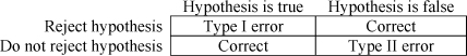
A type I error is rejecting a true hypothesis. A type II error is failing to reject a false hypothesis. These concepts are summarized in the table on the right. It is imprecise to say, “We accept the hypothesis,” because it might be possible to reject the hypothesis with a larger sample size. It is more precise to say, “We are not able to reject the hypothesis based on the data collected so far.”

Some authors define a Type III error as working on the wrong problem.

See consumer’s risk, producer’s risk.

tyranny of the urgent – A time management concept popularized by Hummel (1967) suggesting that people are often so driven by urgent tasks, that they never get around to the important ones.

See Getting Things Done (GTD), Personal Operations Management, two-minute rule, two-second rule.

U

u-chart – A statistical quality control chart used to monitor the number of defectives in a batch, where the batch size may not be constant.

Unlike the c-chart, the u-chart does not require that the batchsize be constant. Like the c-chart, the u-chart relies on the Poisson distribution.

See c-chart, control chart, Poisson distribution, Statistical Process Control (SPC).

unfair labor practice – A term used in the U.S. to describe actions taken by employers or unions that violate the

National Labor Relations Act (NLRA) and administers by the National Labor Relations Board (NLRB).

The NLRA makes it illegal for employers to (1) interfere with two or more employees acting in concert to protect rights provided for in the Act, whether or not a union exists, (2) dominate or interfere with the formation or administration of a labor organization, (3) discriminate against employees for engaging in concerted or union activities or refraining from them, (4) discriminate against an employee for filing charges with the NLRB or taking part in any NLRB proceedings, and (5) refuse to bargain with the union that is the lawful representative of its employees.

Similarly, the NLRA bars unions from (1) restraining or coercing employees in the exercise of their rights or an employer in the choice of its bargaining representative, (2) causing an employer to discriminate against an employee, (3) refusing to bargain with the employer of the employees it represents, (4) engaging in certain types of secondary boycotts, (5) requiring excessive dues, (6) engaging in featherbedding (requiring an employer to pay for unneeded workers), (7) picketing for recognition for more than thirty days without petitioning for an election, (8) entering into “hot cargo” agreements (refusing to handle goods from an anti-union employer), and (9) striking or picketing a health care establishment without giving the required notice.

See human resources.

uniform distribution – A probability distribution for modeling both continuous and discrete random variables.

The continuous uniform is for random variables that can take on any real value in the range (a, b). For example, the continuous uniform can be used to model the clock time for a random arrival during a time interval. The discrete uniform is constrained to integer values and is useful when items are selected randomly from a set.

Parameters: Range (a, b). The a parameter is the location parameter and b – a is the scale parameter.

Density and distribution functions: The continuous uniform distribution is defined in the range (a, b) and has density and distribution functions:

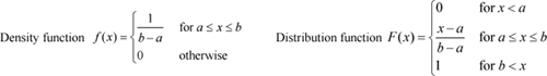
Statistics: The mean and variance of the continuous uniform are μ = (a + b)/2 and σ² = (b − a)²/12. The mean and variance for the discrete uniform are μ = (a + b)/2 and σ² = ((b − a + 1)² − 1)/12. Note that the variances for the continuous and discrete uniform distributions are not the same.

Graph: The graph on the right is the density function for the continuous uniform (1, 2) distribution.

Excel: Excel does not have density or distribution functions for the uniform distribution, but it can be easily implemented using the above equations.

Excel simulation: A continuous uniform random variate in the range (A,B) can be generated in Excel with =A+RAND()*(B-A). A discrete uniform random variable in the range (a, b) can be generated with either RANDBETWEEN(A,B) or A+Int((B-A+1)*RAND()).

See inverse transform method, probability density function, probability distribution.

unit fill rate – See fill rate.

unit of measure – The standard method for counting an item used for inventory records and order quantities; sometimes abbreviated U/M.

The unit of measure is an attribute of each item (stock keeping unit, part number, material) and is stored in the inventory master. Typical values are box, case, pallet, or each. The commonly used term “each” means that each individual item is one unit. The unit of measure can be ambiguous when a box is inside a box, which is inside another box. Typical abbreviations include case (CA or CS), pallets (PL), pounds (LB), ounces (OZ), linear feet (LF), square feet (SF), and cubic feet (CF). Information systems often need to convert the unit of measure. For example, a firm might purchase an item in pallets, stock it in cases, and sell it in “eaches” (units).

See aggregate inventory management, part number, production planning.

Universal Product Code (UPC) – The standard barcode symbol for retail packaging in the U.S.

A UPC is a product identification number that uniquely identifies a product and the manufacturer. It is a series of thick and thin vertical bars (lines) printed on consumer product packages. All UPC identifiers have an associated numeric 12-digit code. The UPC barcode can be scanned at the point-of-sale to enable retailers to record data at checkout and transmit this data to a computer to monitor unit sales, inventory levels, and other factors. Data items can include the SKU, size, color.

The EAN is the international version of the UPC and has 13 rather than 12 digits. EAN stands for European Article Number. When it was introduced, the idea was to expand the UPC across the world with this new code, while still being UPC compliant. To do this, a prefix number was added to the UPC, where the prefix 0 was reserved for existing UPCs. Many firms that import from around the world use both UPCs and EANs in their information systems.

See barcode, Electronic Product Code (EPC), part number, Point-of-Sale (POS), Radio Frequency Identification (RFID).

unnecessary waste – See 8 wastes.

upstream – A manufacturing and supply chain term referring to any process that comes before a given process.

This term makes an analogy between a stream or a river and a manufacturing or supply chain system. Just as water moves downstream, the product flows “downstream.” A downstream process is any process that comes after a given process. Therefore, if the painting process comes after the molding process, the painting process is said to be downstream from the molding. Likewise, an “upstream” process is one that comes before. Therefore, the molding process is said to be “upstream” from the painting process.

See bullwhip effect, Design Structure Matrix (DSM), Drum-Buffer-Rope (DBR), pacemaker, process map, reverse logistics.

utilization – The percentage of the available work time that a resource is working.

Utilization is the ratio of the actual time worked for a resource to the time available. Utilization is a fundamental concept in operations management, capacity management, and queuing theory. It is also one of the three elements of the Overall Equipment Effectiveness (OEE) metric. In queuing theory, utilization is defined as the ratio of the average arrival rate to the average service rate. See the queuing theory entry for more detail.

Operations managers sometimes seek to maximize productivity by maximizing utilization to amortize fixed costs over more units. However, maximizing utilization is often a foolish strategy because high utilization can also mean high inventory, long customer waiting time, and poor customer service. The ideal utilization, therefore, will minimize the sum of the waiting and capacity costs. For example, the ideal utilization for a fire engine is close to zero because the waiting cost is very high. The capacity entry discusses these issues further.

In a factory context, most organizations consider setup time to be part of the work time when calculating utilization. However, the Theory of Constraints (TOC) literature defines utilization as the ratio of the run time (excluding setup time) to the time the resource is scheduled to produce.

See bottleneck, capacity, cellular manufacturing, efficiency, operations performance metrics, Overall Equipment Effectiveness (OEE), productivity, queuing theory, Theory of Constraints (TOC), wait time.

V

validation – See process validation.

validation protocol – See process validation.

value added ratio – The ratio of the processing time (direct value-adding time) to the total cycle time (throughput time); also called Manufacturing Cycle Effectiveness (MCE), throughput ratio, and cycle time efficiency.

In a manufacturing context, the total cycle time (throughput time) is the total time in the system, which usually includes the queue time (wait time), run time, post-operation wait time, and move time. The value-adding time is the “touch time” plus time spent in other value-adding operations, such as baking in an oven, curing, drying, etc. In labor-intensive manufacturing operations, the value-adding time is just the “touch time.” In a service context, the value added ratio is often defined as the percentage of the time that the customer is receiving actual value-added service divided by the time that the customer is in the system. In this author’s experience, most manufacturing plants have a value added ratio far less than 20%.

See batch-and-queue, cellular manufacturing, cycle time, labor intensive, lean thinking, Overall Equipment Effectiveness (OEE), queuing theory, time-based competition, touch time, wait time.

Value Added Reseller (VAR) – An organization that adds value to a system and resells it.

For example, a VAR could purchase computer components (e.g., CPU, motherboard, case, and monitor) and graphics software from a number of different suppliers and package them together as a specialized CAD system. Although VARs typically only repackage and sell products, they might also include software or services they have developed themselves. Adapted from www.pcmag.com/ encyclopedia_term, October 25, 2006.

See Original Equipment Manufacturer (OEM).

value analysis – See value engineering.

value chain – A model developed by Michael Porter that describes the activities in a business that deliver value to a market; this model is used as the basis for a competitive analysis called a value chain analysis.

As shown in the figure below, Porter (1985) suggest business activities can be grouped into primary and support activities⁶¹. Primary value chain activities are those that are directly concerned with creating and delivering a product (e.g., component assembly). Support value chain activities are not directly involved in production but may increase effectiveness or efficiency (e.g., human resource management).

Porter’s value chain

Adapted by Professor Arthur V. Hill from Porter (1985)

A good profit margin is the result of well-designed primary and secondary value chain activities. The firm’s margin or profit depends on how well the frim’s primary activities add value to the market so that the amount that the customer is willing to pay exceeds the cost of the activities in the value chain. It is rare for a business to undertake all primary and support activities for itself. In fact, one of the main benefits of a value chain analysis is to consider which activities should be outsourced to other firms. A competitive advantage can often be achieved by reconfiguring the value chain to provide lower cost or better differentiation.

Primary value chain activities include:

• Inbound logistics – All relationships with suppliers, including all activities required to receive, store, and disseminate inputs.

• Operations – All activities required to transform inputs into outputs (products and services).

• Outbound logistics – All activities required to collect, store, and distribute the output.

• Marketing and sales – All activities to inform buyers about products and services, induce buyers to purchase them, and facilitate their purchase.

• After sales service – All activities required to keep the product or service working effectively for the buyer after it is sold and delivered.

Support value chain activities include:

• Procurement – Acquisition of inputs, or resources, for the firm.

• Human resource management – All activities involved in recruiting, hiring, training, developing, compensating, and (if necessary) dismissing personnel.

• Technological development – Equipment, hardware, software, procedures, and technical knowledge brought to bear in the firm’s transformation of inputs into outputs.

• Infrastructure – Serves the company’s needs and ties the various parts together. Infrastructure consists of functions or departments, such as accounting, legal, finance, planning, public affairs, government relations, quality assurance, and general management.

Porter suggests that firms can gain competitive advantage through either cost leadership or differentiation. In a cost leadership strategy, a firm sets out to become the low-cost producer in its industry. The sources of cost advantage are varied and depend on the structure of the industry. They may include the pursuit of economies of scale, proprietary technology, preferential access to raw materials, and other factors. In a differentiation strategy, a firm seeks to be unique in its industry along some dimensions that are widely valued by buyers. It selects one or more attributes that many buyers in an industry perceive as important, and then uniquely positions itself to meet those needs. It is rewarded for its uniqueness with a premium price.

Value chain analysis can be broken down into three steps:

• Break down a market/organization into its key activities under each of the major headings in the model.

• Assess the potential for adding value via cost advantage or differentiation, or identify current activities where a business appears to be at a competitive disadvantage.

• Determine strategies built around focusing on activities where competitive advantage can be sustained.

Many authors now use the terms value chain and supply chain almost interchangeably. However, most scholars make a distinction between the terms. The value chain takes a business strategy point of view, considers product design and after sales service, and emphasizes outsourcing decisions based on core competencies. In contrast, supply chain management usually takes a materials and information flow point of view and emphasizes suppliers, inventories, and information flow as shown in the SIPOC Diagram and the SCOR model.

See bullwhip effect, delegation, division of labor, human resources, lean sigma, logistics, SCOR Model, SIPOC Diagram, supply chain management, value stream.

value engineering – An approach for designing and redesigning products and services to achieve the same functionality at less cost or achieve better functionality at the same cost; also known as value analysis.

Value engineering techniques (1) identify the functions of a product or service, (2) establish a worth for each function, (3) generate alternatives through the use of creative thinking, and (4) select alternatives to reliably fulfill the needed functions to achieve the lowest life cycle cost without sacrificing safety, quality, or environmental attributes of the project. Value engineering is usually conducted by a multi-disciplined team and applies a well-developed methodology. Value engineering is closely related to product simplification, which is the process of finding ways to reduce product complexity without sacrificing important functionality. Value engineering is also closely related to commonality, which involves using common parts across many products.

See commonality, Design for Manufacturing (DFM), product life cycle management.

value proposition – A statement of the benefits offered by a product or service to a market.

The value proposition is a statement of how a bundle of products and services propose to add value to a set of customers and how that value is differentiated from competitors’ offerings. In an economic sense, the value proposition is the difference between the life-cycle benefits and the life-cycle cost.

See service guarantee, strategy map.

value stream – A lean term used to describe the series of steps (both value-adding and non-value-adding) required to create a product, a product family, or a service.

A value stream includes product and service flows that have similar process steps. A value stream takes a process view focusing on product flows across organizational boundaries. Identifying value streams and creating a value stream map for each one is a good starting point for lean process improvement. This activity can be used to help find and prioritize the non-value-adding steps.

See functional silo, lean thinking, product family, value chain, value stream manager, value stream map.

value stream manager – A lean manufacturing term for an individual who has been assigned the responsibility for a value stream; also called value stream leader.

The value stream may be on the product or the business level.

See lean thinking, value stream, value stream map.

value stream map – A simple process mapping methodology developed at Toyota Motor Company that highlights waste in a system.

Value stream mapping was popularized in the English-speaking world by the Lean Enterprise Institute in the book Learning to See (Rother, Shook, Womack, & Jones 2003). Value stream mapping is a visual tool that graphically identifies every process in a product’s flow from “door-to-door,” giving visibility to both the valueadding steps as well as the non-value-adding steps. The processes that create value are thoroughly detailed for complete process flow of a particular product or product family. The current state is drawn from observation and data gathering of the actual processes. This exercise exposes the waste and redundancy. The future state map is based on lean principles and world-class benchmarks. Value stream analysis activities include:

• Review demand profile (Pareto Chart, histogram)

• Conduct flow analysis (parts process matrix, spaghetti diagram)

• Calculate takt time (peak demand, average demand)

• Create the value stream map (material and information flow diagram using the “learning to see” format, current state and future state gap analysis)

• Identify change loops, kaizen breakthroughs, and the implementation plan.

The diagram below is a simple example of a value stream map created by the author.

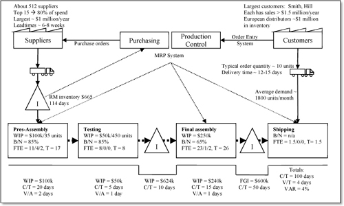
Source: Professor Arthur V. Hill

The data associated with each step can include:

• C/T = Average cycle time.

• V/A = Value-added time or the percentage of total time that is value-added time.

• C/O = Changeover time from one product to another.

• B/N = Bottleneck utilization.

• U/T = The time that the process is available for work or the percentage of the total time that the process is available for work.

• FPY = First pass yield, which is the percentage of the time that the quality standards are met the first time a product goes through the process.

• FTE = Number of full-time equivalent workers required for this process.

The benefits claimed for value stream mapping include:

• Helps users identify and eliminate waste.

• Creates a vision of the future by uncovering wastes and opportunities to create flow.

• Enables broad participation.

• Improves understanding of product cost.

• Helps reduce work in process.

• Helps reduce cycle time.

• Focuses on customer pull signals.

The standard reference on value stream maps is the book Learning to See Version by Rother, Shook, Womack, and Jones (2003).

See A3 Report, causal map, deliverables, lean sigma, lean thinking, process map, value stream, value stream manager.

values statement – See mission statement.

variable costing – An accounting method that defines product cost as the sum of the costs that vary with output and ignores all fixed overhead costs; this usually includes only direct materials and direct labor and possibly the variable portion of manufacturing overhead.

With variable costing, the contribution margin is sales revenue minus variable costs.

See absorption costing, Activity Based Costing (ABC), overhead, standard cost, Theory of Constraints (TOC), throughput accounting.

variance – (1) In a statistics context: A measure of the dispersion (variability) of a random variable; the average squared deviation from the mean; the standard deviation squared. (2) In an accounting context: The difference between the budgeted (planned) and actual amount.

The discussion here is only for the statistics definition. Given a set of n observations on a random variable labeled (x₁, x₂, ... , x_n), the sample variance is defined as .

The first expression is known as the definitional form and the second expression is known as the computational form because it is easier for computing purposes. The computational form requires only “one pass” on the data.

The sample standard deviation is the square root of the sample variance. The population variance and population standard deviation have a denominator of n instead of n−1. Most authors use either the symbol . (sigma hat) or s for the standard deviation of a sample, whereas the σ (sigma) is used for the standard deviation of the population. The unit of measure for the standard deviation is always the same as the raw data and the mean. The inflection points for the normal distribution are at the mean plus and minus one standard deviation. A rough estimate for the standard deviation of a random variable is the range divided by six. The standard deviation for a normally distributed random variable is theoretically equal to , which is approximately 1.25MAD, where the Mean Absolute Deviation . This is true asymptotically⁶², but will almost never be exactly true for any given sample.

In Excel, the formulas for the sample standard deviation and variance are STDEV(range) and VAR(range), and for the population standard deviation and variance they are STDEVP(range) and VARP(range). The Excel formula for the sample covariance is (n/(n−1))*COVAR(x_range, y_range), and the population covariance is COVAR(x_range, y_range).

The variance of the product of a constant a and random variable X is VAR(aX) = a²VAR(X). The variance of the sum of two random variables X and Y is Var(X + Y) = Var(X) + Var(Y) + 2Cov(X, Y). The variance of the weighted sum of two random variables is Var(aX + bY) = a² Var(X)+b² Var(Y) + 2abCov(X, Y). If Y is the sum of N random variables, then .

See Analysis of Variance (ANOVA), correlation, covariance, kurtosis, Mean Absolute Deviation (MAD), mean squared error (MSE), standard deviation.

VAT analysis – A Theory of Constraints classification system used to describe different types of general materials flows and their related bill of material structures.

The shape of each of the letters V, A, and T describes the process flow (Goldratt 1990):

• V-plant – A V-plant transforms a few inputs into a wide variety of products in a “one to many” product flow. This type of process should be master scheduled at the raw materials level. The primary problem in V-plants is allocating the material properly to competing products.

• A-plant – An A-plant transforms (often assembles) a wide variety of inputs into a small variety of final products in a “many to one” product flow. This type of process should be master scheduled at the finished products level. The primary problem in A-plants is synchronizing the incoming materials so that all materials are available when needed.

• T-plant – A T-plant builds standard parts up to a certain point (the crossbar of the “T”) and then assembles these into a wide variety of end products. The components for the lower part of the “T” are built to inventory and then “mixed and matched” in a wide variety of ways for a customer order. Examples include appliances (“white goods”) and computers that have many standard inputs but can result in a variety of end items. This type of process should be master scheduled at the finished components level. T-plants suffer from both synchronization problems of A-plants (parts are not all available for an assembly) and the stealing problems of V-plants (one assembly steals parts that could have been used in another).

Wikipedia lists the fourth process type as an I-plant, which is a simple linear process, such as an assembly line. The primary work is done in a straight sequence of events. The constraint is the slowest operation.

The terms V-plant, A-plant, and T-plant are probably not the best terms and are not commonly used. In this author’s point of view, these terms are a better description of the bill of material than of the plant.

The Master Production Schedule (MPS) entry provides much more detail on this subject.

See bill of material (BOM), Master Production Schedule (MPS), standard parts, Theory of Constraints (TOC), white goods.

VBA – See Visual Basic for Applications (VBA).

Vehicle Scheduling Problem (VSP) – An extension of the Traveling Salesperson Problem (TSP) that can involve multiple vehicles, time window constraints on visiting each node, capacity constraints on each vehicle, total distance and time constraints for each vehicle, and demand requirements for each node.

See the Traveling Salesperson Problem (TSP) entry for more detailed information.

See milk run, Traveling Salesperson Problem (TSP).

vendor – See supplier.

vendor certification – See supplier qualification and certification.

vendor managed inventory (VMI) – A supplier-customer relationship where the vendor assumes responsibility for managing the replenishment of stock; also known as supplier-managed inventory (SMI).

In a traditional supplier-customer relationship, a customer evaluates its own inventory position and sends an order to a supplier (vendor) when it has a need for a replenishment order. With VMI, the supplier not only supplies goods, but also provides inventory management services. The supplier-customer agreement usually makes the supplier responsible for maintaining the customer’s inventory levels. For VMI to work, the supplier needs to have access to the customer’s inventory data. Examples of VMI in practice for many years include:

• Supermarkets and vending machines have used this concept for decades.

• Frito-Lay’s route salespeople stock the shelves for their retail customers to keep the product fresh and the paperwork simple. Much fresh produce moves into convenience shops in the same way.

• For more than 20 years, Hopson Oil, a home heating oil supplier, has automatically scheduled deliveries for fuel oil based on consumption forecasts for each customer. In this way, it keeps its order-taking costs down and keeps the process simple for customers.

Rungtusanatham, Rabinovich, Ashenbaum, and Wallin (2007) define consignment as supplier-owned inventory at the customer’s location and reverse consignment as customer-owned inventory at the supplier’s location. (See the table below.) They further define “Vendor-Owned Inventory Management” (VOIM) as supplier-owned inventory at the customer location (consignment inventory), but managed by the supplier. The table below calls this “Consignment VMI.”

Inventory management alternatives

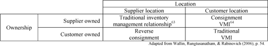
The advantages and disadvantages of VMI over a traditional purchasing relationship are listed below.

Advantages and disadvantages of VMI compared traditional supplier customer relationships

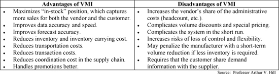
VMI is relatively easy to implement from a technical perspective because the computer hardware and software tools are readily available. However, job functions, processes, and performance measurements all need to change in order to get the most benefit.

Like other customer interface strategies, VMI has strategic implications. The fundamental value proposition is one where the supplier is able to reduce the transaction cost for the customer, but at the expense of increasing the customer’s switching cost (the cost to switch from one supplier to another).

See co-location, consignment inventory, delegation, inventory management, JIT II, outsourcing, purchasing, replenishment order, supply chain management, switching cost.

Version control – The process of keeping track of changes to software, engineering specifications, product designs, databases, and other information; also known as revision control.

Version control is commonly used in software development, product design, engineering, and architecture, where multiple people may change the same set of files. Changes are usually identified by an alphanumeric code called the revision number, revision level, or version number. For example, the initial design might be labeled revision 1, but when a change is made, the new version is labeled revision 2. Each revision should identify the date and the person who made the change. Ideally, revisions can be compared, restored, and merged. Software version control tools and disciplines are essential for all multi-developer projects.

See Engineering Change Order (ECO), Product Data Management (PDM), product life cycle management.

Vertical integration – The process a firm uses to acquire sources of supply (upstream suppliers) or channels of distribution (downstream buyers).

Because it can have a significant impact on a business unit’s position in its industry with respect to cost, differentiation, and other strategic issues, the vertical scope of the firm is an important strategic issue. Expansion of activities downstream is referred to as forward integration and expansion upstream is backward integration. The table below compares the potential advantages and disadvantages of a firm becoming more vertically integrated.

Evaluation of vertical integration

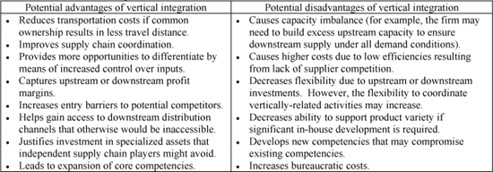
Some situational factors favoring vertical integration include:

• Taxes and regulations on market transactions

• Obstacles to the formulation and monitoring of contracts

• Strategic similarity between the vertically related activities

• Sufficiently large production quantities so the firm can benefit from economies of scale

• Reluctance of other firms to make investments specific to the transaction

The following situational factors tend to make vertical integration less attractive:

• The quantity required from a supplier is less than the minimum efficient scale for producing the product.

• The product is a commodity and its production cost decreases significantly as cumulative quantity increases.

• The core competencies between the activities are very different.

• The vertically adjacent activities are in very different types of industries. For example, manufacturing is very different from retailing.

• The addition of the new activity places the firm in competition with another player with which it needs to cooperate. The firm may then be viewed as a competitor rather than as a partner.

Alternatives to vertical integration may provide many of the same benefits without the risks. Some of these alternatives include long-term explicit contracts, franchise agreements, joint ventures, and co-location of facilities (Greaver 1999). Some of the above ideas are adapted from quickmba.com/strategy/vertical-integration.

See joint venture, make versus buy decision, operations strategy, outsourcing, supply chain management.

virtual organization – A business model where the selling organization is able to pull together business partners to satisfy a customer order, launch a new product, or supply a product to a market without owning many of the key components of the system.

Virtual organizations have significant flexibility benefits, but given the tenuous nature of their relationships, they may not be sustainable. Many high-technology development firms design products and then find contract manufacturers to build them and distributors to find markets for them.

See agile manufacturing, mass customization, operations strategy, organizational design.

virtual teams – Groups that do not meet in person but use technologies such the Internet to communicate.

vision statement – See mission statement.

Visual Basic for Applications (VBA) – A programming language built into most Microsoft Office applications.

VBA makes it possible to write user-defined functions and programs in Microsoft Excel. VBA code is sometimes referred to as a “macro.” The example on the right shows VBA code for a user-defined function that multiplies the input by two. Winston and Albright (2011) provide excellent instruction on VBA programming and modeling.

visual management – See visual control.

visual control – A lean manufacturing approach of designing systems that give everyone in a work area immediate information about the current status of a system.

Visual controls are simple, easy-to-see clues that give managers and workers immediate information about the current status of a system. Visual control requires that the normal and abnormal states be immediately apparent. As Jerome Hamilton of 3M says, “My shop floor speaks to me.” Although many computer-based information systems make use of exception reports and “traffic light” reports (with red, yellow, and green fields), most of them do not meet lean standards for truly visual communication of the system status. Examples of visual control include (1) a shadow board that clearly and quickly shows, which tools are missing, (2) an andon light that clearly shows when a worker is having trouble, and (3) work stoppage in a pull system.

See 5S, andon light, lean thinking, shadow board.

VMI – See vendor managed inventory.

VOC – See voice of the customer (VOC).

voice of the customer (VOC) – Customer opinions, perceptions, desires (both stated and unstated), and requirements.

It is important for organizations to understand both internal and external customers’ needs and desires as they change over time. This voice of the customer should inform both new product development and process improvement efforts. Quality Function Deployment (QFD) is a tool that can be used to translate the voice of the customer into product features and specifications. The VOC is considered one of the keys to success for process improvement programs and projects.

The voice of the customer can be captured in a variety of ways such as:

• Interviews

• Customer satisfaction surveys

• Market research surveys

• E-surveys

• Comment cards

• Focus groups

• Customer specifications

• Contractual requirements

• Observation

• Warranty and service guarantee data

• Field reports

• Complaint logs

• Customer loyalty (i.e., repeat sales)

• Exploratory marketing (Hamel & Prahalad 1991)

Many of the entries listed below discuss specific VOC tools.

See Analytic Hierarchy Process (AHP), critical incidents method, Critical to Quality (CTQ), Customer Relationship Management (CRM), ethnographic research, Kano Analysis, lean sigma, New Product Development (NPD), Process Improvement Program, Pugh Matrix, Quality Function Deployment (QFD), quality management, Voice of the Process (VOP).

Voice of the Process (VOP) – Communication from the system (process) to the process owner.

Process owners receive two important sources of information: the voice of the customer (VOC) and the Voice of the Process (VOP). Whereas the VOC communicates customer desires, requirements, needs, specifications, and expectations, the VOP communicates information about the performance of the process. The VOP can use many quality tools, such as bar charts, Pareto charts, run charts, control charts, cause and effect diagrams, and checksheets. The challenge for the process owner/manager is to use VOP information to better meet the customer needs as defined by the VOC.

See voice of the customer (VOC).

voice picking – A speech recognition system that allows warehouse workers to verbally enter data into a system.

Voice picking is a feature available in many warehouse management systems that allows workers’ hands to be free while working. Benefits include improved accuracy, productivity, accuracy, and reliability.

See picking, warehouse, Warehouse Management System (WMS).

volume flexibility – See flexibility.

V-plant – See VAT analysis.

VSP (Vehicle Scheduling Problem) – See Traveling Salesperson Problem (TSP), Vehicle Scheduling Problem (VSP).

W

Wagner-Whitin lotsizing algorithm – A dynamic programming algorithm for finding the optimal solution for the time-varying demand lotsizing problem.

An implementation of this algorithm (including the pseudocode) can be found in Evans (1985).

See algorithm, lotsizing methods, time-varying demand lotsizing problem.

wait time – A random variable indicating the time that a customer (or an order) is delayed before starting in a process; also called waiting time or queue time.

The wait time is the time that a customer or order is delayed before starting in service. The time in system for a particular customer is the wait time (queue time) plus the service time, and the average time in system is the average wait time plus the average service time. The average queue time and the average time in system are important system performance measures. Wait time (queue time) is often the largest portion of the manufacturing cycle time. In the lean manufacturing philosophy, wait time is considered wasteful.

See cycle time, lean thinking, Little’s Law, operations performance metrics, queuing theory, time in system, turnaround time, utilization, value added ratio, Work-in-Process (WIP) inventory.

waiting line – See queuing theory.

warehouse – A building or storage area used to store materials.

Warehouses are used by manufacturers, importers, exporters, wholesalers, distributors, and retailers to store goods in anticipation of demand. They are usually large metal buildings in industrial areas with loading docks to load and unload goods from trucks, railways, airports, or seaports. Nearly all Warehouse Management Systems (WMS) allow users to define multiple logical warehouses inside a single building.

Warehouses usually use forklifts to move goods on pallets. When a shipment arrives at a warehouse, it must be received and then put away. When a customer order is received, it must then be picked from shelves, packed, and shipped to the customer.

Having a good inventory system is critical to the success of a warehouse. WMSs can help reduce the cost to receive and put away products and reduce the cost to pick, pack, and ship customer orders. A good WMS also improves record accuracy for on-hand, allocated, and on-order quantities.

A zone is an area of a warehouse used for storing one type of product. For example, a hospital inventory might have one zone for forms, another for medical-surgical items, and still another for pharmacy items (drugs). A rack is a storage shelf, usually made from metal. An aisle is a space for people to walk and for materials handling equipment to move between racks. A section or bay is usually the space defined by a pair of upright frames and a shelf (or level) is the level in the section or bay. Finally, a bin (or slot) is a specific storage location (or container) used to store multiple units of a single item. Bins are commonly made of metal, corrugated cardboard, or plastic, and may have a cover. Bins may have capacity limits in terms of weight, volume, or units. Bins are referenced by warehouse, zone, rack (or aisle), bay (or section), shelf (level or row), and bin number. Barcoding bins can reduce cost and increase picking accuracy.

Warehouses must have a locator system to find items. Items may be stored using a fixed location system, a random location system, or a zone location system. Fixed location systems label the shelves with the item (SKU, material) number and attempt to keep products only in that one storage area. In contrast, random location systems label the shelves with the bin (bay) number and shelf number and then use a computer-based system to keep track of what items are stored in each bin. Zone storage is a combination of the two that uses fixed storage areas for groups of items but uses random storage in each zone.

Warehouses can use a variety of slotting rules to guide where an item is stored. Similarly, warehouses can use a variety of picking systems to create a pick list that guides stock pickers in picking (retrieving) materials from the warehouse to fill orders.

Most warehouses use a First-In-First-Out (FIFO) policy for managing physical inventory. However, it is important to note that the accounting system might still use last-in-first-out for costing purposes. Warehouses generally use either pallet rack or carton flow racking. As the names suggest, pallet racks store pallets (or skids) and carton flow racking stores cartons. Pallet racks can be either static or flow racks (gravity rack). Static racks must use LIFO. In contrast, pallet flow racks use gravity so pallets loaded in the rear flow forward on a wheeled track to a picking position. Pallet flow racks, therefore, use FIFO. Carton systems sometimes use wheeled shelves and conveyors to move products and sometimes use gravity flow.

A public warehouse is a business that leases space and provides services to customers, usually on a month-to-month basis, and uses its own equipment and labor to provide warehouse services, such as receiving, storage, and shipping. Public warehouses charge based on space and labor usage. In contrast, a contract warehouse provides warehouse services for a specified period of time (often yearly) where the owner of the goods pays for the space even if it is not used. Both public and contract warehouses are often used to supplement space requirements of a private warehouse.

A bonded warehouse is a facility (or dedicated portion of a facility) where imported goods are stored until custom duties are paid. In the U.S., a bonded warehouse must be approved by the U.S. Treasury Department and under bond/guarantee for observance of revenue laws. A bonded warehouse can be particularly useful when products are received well in advance of sale because the import fees are not usually paid until the products are shipped from the bonded warehouse.

Dry storage is storage of non-refrigerated products, such as canned goods. Cold storage is for perishable food and other products that require refrigeration. Cold storage can be either refrigerated storage (above freezing) or frozen storage (below freezing).

See ABC classification, aggregate inventory management, Automated Storage & Retrieval System (AS/RS), carousel, cross-docking, cube utilization, discrete order picking, distribution center (DC), Distribution Requirements Planning (DRP), dock, facility location, First-In-First-Out (FIFO), flow rack, forklift truck, forward pick area, fulfillment, locator system, logistics, materials management, numeric-analytic location model, pallet, part number, periodic review system, pick face, pick list, picking, pull system, Radio Frequency Identification (RFID), random storage location, receiving, reserve storage area, safety stock, slotting, square root law for warehouses, supply chain management, task interleaving, Third Party Logistics (3PL) provider, voice picking, Warehouse Management System (WMS), wave picking, zone storage location.

Warehouse Management System (WMS) – A software application that helps organizations manage the operations of a warehouse or distribution center.

WMSs manage the storage and retrieval of materials in a building and handle the transactions associated with those movements, such as receiving, put away (stocking), cycle counting, picking, consolidating, packing, and shipping. The WMS guides the operator or machine with information about item locations, quantities, units of measure and other relevant information to determine where to stock, where to pick, and in what sequence to perform each operation. Newer warehouse management systems include tools that support more complex tasks, such as inventory management, product allocations, shipment planning, workforce planning/labor management, and productivity analysis. WMSs can be stand-alone systems, modules in an ERP system, or modules in a supply chain execution suite. The benefits of a good WMS include reduced inventory, reduced labor cost, increased storage capacity, improved customer service, and improved inventory accuracy. Traditionally, WMSs have used barcodes or smart codes to capture data; however, more recently, Radio Frequency Technology (RFID) technology has been added to provide real-time information. However, most firms, especially in manufacturing and distribution, still use barcodes to capture data because of their simplicity, universality, and low cost.

See ABC classification, Advanced Shipping Notification (ASN), Automated Data Collection (ADC), bill of material (BOM), cross-docking, distribution center (DC), Distribution Requirements Planning (DRP), dock-to-stock, fixed storage location, forward pick area, fulfillment, inventory management, locator system, logistics, materials management, Over/Short/Damaged Report, picking, Radio Frequency Identification (RFID), random storage location, real-time, receiving, slotting, slotting fee, task interleaving, Transportation Management System (TMS), voice picking, warehouse, wave picking, zone picking, zone storage location.

warranty – A guarantee given from the seller to the purchaser stating that a product is free from known defects and that the seller will repair or replace defective parts within a given time limit and under certain conditions.

A warranty and a service guarantee have identical legal obligations for the seller. The difference is that a warranty is for a product (a tangible good) and a service guarantee is for a service (an intangible product). Blischke and Murty (1992) and Murty and Blischke (1992) provide a good summary of the warranty literature.

See caveat emptor, product design quality, service guarantee, Service Level Agreement (SLA).

waste – See 8 Wastes.

waste walk – The lean practice of walking through a place where work is being done to look for wasteful activities; also called a gemba walk.

When conducting a waste walk, it is wise to engage with the gemba, ask the “5 Whys,” take notes as you go, and follow-up as necessary.

See 3Gs, 8 Wastes, gemba, lean thinking, management by walking around.

water spider – A lean manufacturing practice of assigning a skilled worker to re-supply parts to the point of use on the production line; a worker who follows a timed material delivery route; also known as mizusumashi (in Japanese), water strider, water beetle, water-spider, or material delivery route.

The water spider’s job is to follow the schedule and maintain the inventory on a production line between a minimum and maximum level. They typically use a cart to deliver materials to workstations in predefined quantities at least every one to two hours on a fixed time schedule. This ensures that the manufacturing line has the right amount of inventory at the right time. Compared to traditional methods, material delivery routes stock line bins more frequently and in smaller quantities, resulting in reduced WIP inventory and reduced waiting time.

The water spider has a routine and knows all processes thoroughly enough to step in if needed. Water spiders sometimes also assist with changeovers, provide tools and materials, and provide other help needed to maintain flow. At Toyota, performing the water spider role is a prerequisite for supervisory positions.

The water spider is named after the whirligig beetle that swims about quickly in the water. The Japanese word for water spider is mizusumashi, which is written as in Kanji (source: www.babylon.com/definition/mizusumashi/Japanese, December 28, 2009).

See lean thinking, point of use.

waterfall – See waterfall scheduling.

waterfall scheduling – (1) A project management approach that does not allow a step to be started until all previous steps are complete. (2) A lean methodology that schedules customers to arrive every few minutes.

Definition (1) – The project management context: In a waterfall process, steps do not overlap. The Gantt Chart for a waterfall process looks like a waterfall, with each step starting after the previous step. The term is often used in a software development context where the design step is not allowed to begin until the requirements step is complete, the coding step is not allowed to begin until the design step is complete, etc. This waterfall scheduling process only works well in situations where the domain is fully specified, well structured, and well understood. However, in the software development context, the term “waterfall process” is often used to criticize old thinking that does not allow for iterative, spiral, lean, and agile development approaches.

Definition (2) – The customer scheduling context: Some lean healthcare consultants use the term “waterfall scheduling” to mean scheduling patients to arrive every few minutes (e.g., 10 or 15 minute intervals) rather than in batches every half-hour. Batch arrivals cause bottlenecks for receptionists and nurses and cause long waits for many patients. Therefore, waterfall scheduling in this context is a positive thing, because it spreads out arrivals and develops a smooth even flow for the service process.

Although both of the above definitions have to do with scheduling, they are used in different contexts. Definition (1) is usually presented as a bad practice, and definition (2) is usually presented as a good practice.

See agile software development, concurrent engineering, Gantt Chart, New Product Development (NPD), project management, scrum, sprint burndown chart, stage-gate process, transactional process improvement.

wave picking – A method of creating a pick list where all items for a particular group of orders (e.g., a carrier, destination, or set of work orders) are picked and then later grouped (consolidated) by ship location.

With wave picking, all zones are picked at the same time, and the items are later sorted and consolidated to fill individual orders. The principle is to handle each item efficiently two times, rather than inefficiently once. A wave is a grouping of orders by a specific set of criteria, such as priority level, freight carrier, shipment type, or destination. These orders are released to the different zones in the warehouse as a group. Clearly, the rate for each of the two handling steps, batch picking and container loading (consolidation), must be considerably more than twice as fast as the single step in traditional serial order picking to make wave picking worthwhile.

The two options for wave picking include fixed-wave picking and dynamic-wave picking. With fixed-wave picking, orders are not sent off to be packed until the entire wave’s worth of items has been picked. With dynamic-wave picking, each order is sent to the packer as it is completed.

Operations with a high total number of SKUs and moderate to high picks per order may benefit from wave picking. Although wave picking is one of the quickest methods for picking multiple line orders, some distribution centers struggle with order consolidation, sorting, and verifying that the contents are correct.

See batch picking, distribution center (DC), picking, warehouse, Warehouse Management System (WMS), zone picking.

waybill – A shipping document created by a carrier identifying the shipper, date of shipment, carrier, number of parcels, weight, receiver, and date received; also called an air waybill, Air Consignment Note.

The waybill confirms receipt of the goods by the carrier. Unlike a bill of lading, which includes much of the same information, a waybill is not a document of title.

See bill of lading, Cash on Delivery (COD), FOB, terms, Transportation Management System (TMS).

WBS – See work breakdown structure.

weeks supply – See periods supply.

Weibull distribution – A continuous probability distribution for modeling lifetimes of objects, time to failure, or time to complete a task that has a long tail; a probability distribution that is commonly used in reliability theory and maintenance for extreme values.

Parameters: Shape parameter α > 0 and scale parameter β > 0. Some sources add a location parameter γ by replacing x with (x − γ). (Note: The reliability literature uses shape and scale parameters and β and η.)

Density and distribution functions: The density and distribution functions for x > 0 are f(x) = αβ^−α x^α−1 exp(−(x/β)^α) and F(x) = 1 −exp(−(x/β)^α).

Statistics: Range [0, ∞), mean βΓ(1+1/α), median βIn(1)^1/α, mode β((α − 1)/α)^1/α if α 1 and otherwise, variance (β²/α)(2Γ(2/α) − 1(1/α)Γ(1/α)²) where Γ() is the gamma function.

Graph: The graph on the right shows the Weibull density function with (α, β) = (2, 1).

Parameter estimation: Estimating the α and β parameters from a set of observations requires numerical methods for both the MLE and method of moments estimators. See Law and Kelton (2000) for information on the MLE approach.

Excel: In Excel, the Weibull density and distribution functions are WEIBULL(x, α, β, FALSE) and WEIBULL(x, α, β, TRUE). Excel 2003/2007 has no inverse function for the Weibull, but it can be calculated with the Excel formula x = β*(-ln(1-F(x)))^(1/α). Excel 2010 renamed the function WEIBULL.DIST, but it still uses the same arguments.

Excel simulation: In an Excel simulation, Weibull distributed random variates can be generated with the inverse transform method using x = β*(-ln(RAND()))^(1/α).

Relationships to other distributions: The exponential distribution is a special case of the Weibull when α = 1, and the Rayleigh distribution is a special case of the Weibull distribution when α = 2. When α = 3, the Weibull distribution is similar to the normal distribution.

History: The Weibull distribution was named after Swedish engineer and scientist Ernst Hjalmar Waloddi Weibull (1887-1979) (source: www.wikipedia.org, November 20, 2007.)

See bathtub curve, beta distribution, exponential distribution, inverse transform method, probability density function, probability distribution, Total Productive Maintenance (TPM).

weighted average – An average where some values contribute more than others.

A weighted average is commonly used in forecasting where it is important to give more weight to more recent data. Mathematically, a weighted average is , where T is the number of values (time periods), t is the period index, w_t is the weight assigned to the value in period t, x_t is the value in period t, and . The weights are often required to sum to one, which simplifies the equation to .

See carrying charge, carrying cost, exponential smoothing, forecast error metrics, moving average, periods supply.

Weighted MAPE – See Mean Absolute Percent Error (MAPE).

what-if analysis – The practice of evaluating the results of a model when input parameters are changed.

What-if sensitivity analysis is often done with mathematical optimization, stochastic simulation, and queuing theory models to help decision makers (1) evaluate different potential scenarios and make risk return trade-offs, (2) refine their intuition about the relationships in the model, and (3) validate that the model fits the real-world.

See Activity Based Costing (ABC), DuPont Analysis, linear programming (LP), queuing theory, simulation.

where-used report – A listing of all materials that are “parents” for a particular material in a bill of material.

See bill of material (BOM), bill of material implosion, Materials Requirements Planning (MRP), pegging.

white goods – Major electric appliances (machines) that are typically finished in white enamel.

Examples of white goods include refrigerators, freezers, dishwashers, stoves, ovens, washing machines, dryers, and water heaters. White goods are usually classified as consumer durables, but can be sold for either consumer or commercial uses.

See durable goods, platform strategy, private label, VAT analysis.

wholesale price – See wholesaler.

wholesaler – A distributor that buys goods and resells them to organizations other than final customers; also called a distributor or jobber.

Wholesalers often buy large quantities of goods from manufacturers, store them in warehouses, and sell them to retailers who sell to consumers. The wholesale price is the price wholesalers pay when buying in large quantities. A rack jobber is a wholesaler that provides goods on consignment for rack displays in retail locations. They are given dedicated space in the store in exchange for sharing profits with the retailer.

See B2B, broker, distributor, supplier, supply chain management.

Winsorizing – A simple bounding procedure that replaces values greater (less) than the maximum (minimum) value allowed with the maximum value.

Data can be Winsorized by setting a maximum and minimum value or by defining the upper and lower percentiles allowed on the cumulative distribution. Whereas Winsorizing replaces values in the tail of the sample, trimming excludes these values.

See forecast error metrics, Mean Absolute Percent Error (MAPE), outlier, Relative Absolute Error (RAE), trim, trimmed mean.

WIP – See Work-in-Process (WIP) inventory.

WMS – See Warehouse Management System (WMS).

work breakdown structure (WBS) – A project management tool that defines the hierarchy of project activities (tasks) needed to complete the project.

The WBS is a useful way to identify all tasks needed for a project, break large tasks into smaller, more manageable tasks, and organize and communicate the list of tasks. The WBS lists all tasks required for the project, starting at the highest level of aggregation and going down to a detailed list of all tasks. It is like a bill of material for the project and can be drawn like the roots of a tree. The WBS does not create the project schedule, communicate precedence relationships between tasks, or define the resources required for each task. The U.S. Air Force encourages suppliers to define a WBS so all tasks require about one week of work.

For example, the top level of the WBS for a wedding might include create invitations, acquire dresses/tuxes, and reserve church. The example below shows a small portion of the WBS for this simple example. This WBS could be broken down into much more detail as needed. The lowest level of the WBS should define all specific tasks needed to complete the project.

It is important to understand that the WBS is not a schedule or sequence of activities. It is simply a hierarchical list of the activities that need to be done to complete the project.

Example work breakdown structure for a wedding

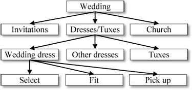
The next step after using the WBS to identify tasks is to identify the precedence constraints between the tasks. That information can then be used to determine the early and late start times and early and late finish times for each task and finally determine the critical path through the network.

See Critical Path Method (CPM), Earned Value Management (EVM), mindmap, Project Evaluation and Review Technique (PERT), project management.

work center – See workcenter.

work design – See job design.

work measurement – The process of estimating the standard time required for a task; also called labor standards, engineered labor standards, labor management systems, and Methods Time Measurement (MTM).

The main reasons for a work measurement system (labor management system) include:

• Cost accounting – Standard times are used to assign both labor and overhead cost to products or jobs.

• Evaluation of alternatives – Standard times are used to help evaluate new equipment investments or changes in the current equipment configuration.

• Evaluation and reward systems – Standard times are often used as a basis of comparison for evaluating and rewarding direct labor, where workers are rewarded when they “beat” the standard times.

• Scheduling – Jobs, workers, and machines are often scheduled based on standard times.

The three common ways to measure the time for a task are (1) time study, (2) standard data, and (3) work sampling. A time study can be used for almost any existing job with a relatively short duration. Standard data only requires that the analyst determine which elemental motions (e.g., pick, drop, etc.) are required for the job. Once these are determined, the analyst simply looks these up in the reference database and adds them up to “assemble” the total time for the task. The data for this type of analysis is often called pre-determined motion and time data. Work sampling takes a large number of random “snapshots” (samples) of the process over several weeks and estimates how much time is spent in each “state” based on the percentage of the random samples found in each state. This data is often self-reported and is more appropriate for knowledge work.

See human resources, job design, normal time, operations performance metrics, overhead, performance management system, performance rating, scientific management, standard time, time study, work sampling.

work order – A request for a job to be done; also called a workorder, job, production order, and work ticket.

In a manufacturing context, a work order is a request to a maintenance organization to perform either preventive or emergency maintenance or a request to a machine shop to make a tool. Work orders should identify the customer, the date the work order was created, and some indication of the urgency of the work.

A work order should not be confused with a manufacturing order.

See maintenance, manufacturing order, Total Productive Maintenance (TPM).

work sampling – The application of statistical sampling methods to estimate the percentage of time that a worker is spending on each activity (or in each “state”); also called occurrence sampling.

This approach to work measurement should only be used for long cycle tasks. For example, a hospital administrator wants to know how much time nurses are sitting at the nursing station per day. The person responsible for collecting the data takes a large number of random “snapshots” (samples) of the process over several weeks. Work sampling assumes that the percentage of the samples in each activity (state) is proportional to the percentage of work time in each activity. From these snapshots, the administrator can estimate how much time nurses spend at the nursing station per day on average.

The advantage of work sampling over other work measurement tools is that the data are gathered over a relatively long time period. In contrast, a time study makes more sense for a task that requires a relatively short amount of time, with the observer recording each repetition of the process.

See normal time, sampling, standard time, time study, work measurement.

work simplification – The process of reducing the complexity of a process.

Work simplification involves designing the job to have fewer stages, steps, moves, and interdependences, thus making the job easier to learn, perform, and understand. This is closely related to work standardization. Although normally applied only to repetitive factory and service work, it can also be applied to less repetitive knowledge work done by professionals and salaried workers. Simplicity is highly valued in lean thinking.

See Business Process Re-engineering (BPR), error proofing, Failure Mode and Effects Analysis (FMEA), human resources, job design, job enlargement, standardized work.

work standardization – See standardized work.

work standards – See standardized work.

workcenter – An area where work is performed by people, tools, and machines and usually focuses on one type of process (e.g., drilling) or one set of products (e.g., assembly of a particular type of product).

A workcenter in a factory is usually a group of similar machines or a group of processes used to make a product family. The item routing defines the sequence of workcenters required to make a product. When a workcenter has multiple machines or people, the production planning system usually considers them identical in terms of capabilities and capacities.

See cellular manufacturing, facility layout, routing.

workflow software – See groupware.

workforce agility – The ability of the employees in a firm to adapt to change.

The main benefits of increased workforce agility can include (Hopp and Van Oyen 2001):

• Improved efficiency – Better on-time delivery, reduced cycle time, and reduced Work in Process (WIP) because idle time in the production line is decreased.

• Enhanced flexibility – Reduced overtime cost, increased productivity, reduced absenteeism and labor turnover because cross-trained workers can absorb some of the work assigned to absent workers.

• Improved quality – Increased worker knowledge which enables them to reduce defects.

• Improved culture – Improved working environment due to increased job satisfaction, worker motivation, and reduced ergonomic stress.

However, it is possible to have too much agility. Workers cannot be expected to be experts at every job in an organization. Training that is never used is of very limited value to the organization. Some specialization is good from a learning curve and responsibility assignment point of view.

See absorptive capacity, cross-training, human resources, job design, job rotation, learning curve, learning organization, organizational design, RACI Matrix.

Work-in-Process (WIP) inventory – Orders or materials that have been started in a production process, but are not yet complete; sometimes called Work-in-Progress inventory and in-process inventory.

Work-in-Process (WIP) includes all orders or materials in queue waiting to be started, in the process of being set up, currently being run, waiting to be moved to the next operation, and being moved. WIP inventory is usually valued as the sum of the direct labor, materials, and overhead for all operations that have been completed. Some factories assign manufacturing overhead to a product when it is started; others assign manufacturing overhead when it is completed. Goldratt recommends not assigning overhead at all.

See blocking, cellular manufacturing, CONWIP, finished goods inventory, Little’s Law, overhead, pipeline inventory, throughput accounting, wait time.

Work-in-Progress inventory (WIP) – See Work-in-Process (WIP) inventory.

X

x-bar chart – A quality control chart that monitors the mean performance of a process.

A sample of n parts is collected from a process at regular intervals (either time intervals or production quantity intervals). The mean of the sample is plotted on the control chart, and the process is evaluated to see if it is “under control.” The name of this chart comes from the sample mean , which is read as “x-bar.”

See control chart, Statistical Process Control (SPC), Statistical Quality Control (SQC).

X-Matrix – See hoshin planning.

XML (Extensible Markup Language) – A simple, flexible language used to create webpages.

XML is an extensible version of Hypertext Markup Language (HTML). Another popular way to create webpages is Active Server Pages (ASP). XML is also a robust and flexible alternative to Electronic Data Interchange (EDI).

See Electronic Data Interchange (EDI), robust.

Y

yield – (1) In manufacturing: The ratio of units started in a process to completed without defect. (2) In finance: The ratio of return to investment. (3) In service management: The ratio of realized to potential revenue.

See the yield management entry for the service management context. See the Compounded Annual Growth Rate (CAGR) and Internal Rate of Return (IRR) entries for the finance context.

In the manufacturing context, process yield (also called final yield) is used as (1) a performance measure (after production) and (2) a planning factor (before production) to increase the production start quantity so the final quantity meets the requirements. Process yield planning factors are usually stored in the bill of material. For example, if the requirement is for 100 units and the process yield is 80%, the start quantity should be 100/0.8 = 125 units so that the final quantity produced is 125 × 0.8 = 100 units.

Lean sigma consultants often promote a demanding yield metric called rolled throughput yield (RTY), sometimes also called first pass yield and first time yield. This is the percentage of units completed without needing any rework. The following table compares the traditional process yield with RTY.

Comparison of traditional process yield and rolled throughput yield (RTY)

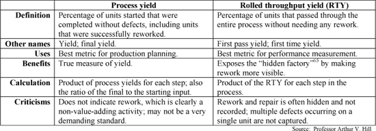
The table below provides a simple example of these metrics. Reporting only the overall process yield of 90% hides the extensive rework in this process; however, the RTY of 25.9% makes the rework evident.

Yield metric example

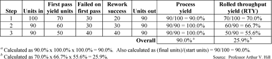
Process yield is one of the three dimensions of Overall Equipment Effectiveness, an important performance measure in many firms. Note that yield has little relationship to yield management tools used in services.

See bill of material (BOM), conformance quality, hidden factory, operations performance metrics, Overall Equipment Effectiveness (OEE), process capability and performance, quality management, scrap, supplier scorecard.

yield management – A set of metrics and tools for maximizing revenue for organizations that have relatively fixed capacity costs; also called revenue management or perishable asset resource management.

The goal – For many capital-intensive businesses, such as airlines, hotels, theaters, stadiums, and utilities, maximizing revenue is equivalent to maximizing profit, because nearly all costs are relatively fixed. The goal is to maximize revenue per unit of resource ($/room night, $/seat mile, etc.). The goal is not to maximize utilization, although that is usually the result.

The control variables – Yield management systems change prices and capacity allocations over time as the date of the event approaches. For example, airlines change their prices thousands of times every day.

The performance metrics – The following yield management terms are used in the airline industry:

Available seat miles (ASM) – A measure of capacity defined as the number of seat miles that are available for purchase on an airline.

Revenue passenger miles (RPM) – The number of available seat miles (ASM) actually sold. This is a measure of an airline’s traffic.

Load factor – The RPM divided by the ASM. Alternatively, this can be measured by the percentage of seats that were sold compared to the number of seats that could have been sold.

Yield – How much an airline makes per revenue passenger mile (RPM).

Revenue per available seat mile (RASM) – Sometimes called the “unit revenue,” this metric has become the industry standard and is tracked each month because it gives a good overall picture of how an airline is performing.

Cost per available seat mile (CASM) – A widely used metric indicating the cost divided by the available miles that could have been flown (not the miles actually flown), regardless if the seats were occupied.

Stage length – The length of the average flight for a particular airline. As stage length increases, costs per mile tend to go down. Consequently, increases in the stage length of an airline will tend to bode well for the cost side, all other things being equal.

The booking curve – See the booking curve entry for more information on this yield management tool.

Other factors – Hotels and airlines place great importance on no-show factors, cancellations/reservation adjustments, and “wash” for groups, all of which help determine the necessary level of “oversell.” Businesses with perishable inventory must remember that when the forecasted demand is below capacity, it is better to sell the room at a lower rate than to not sell it at all. In the hotel business, the term “revenue management” is often equated with getting “heads in beds.” Additional ways to maximize revenues are to implement length of stay or stay restrictions, overbook effectively, take advantage of up-sell opportunities, and allocate correct inventory to the appropriate channels (discounts in particular). An emerging trend in the hotel business is to move all segments, not just e-channels and rack (standard), to dynamic pricing structures. This will enable the hotels to better control the negotiated/volume accounts, which is one of the larger segments.

See booking curve, capacity, congestion pricing.

Y-tree – A tool for creating a strategic linkage between the efforts of individuals and the goals of the organization; also called a goal tree.

The Y-tree begins at the highest level of organizational goals and breaks these down into intermediate goals and objectives, which are finally translated into specific projects. A Y-tree is essentially a strategy map, but goes one step further by connecting the metrics to action plans and projects. Like a strategy map, a Y-tree represents the firm’s hypotheses and beliefs about how the highest-level performance variables are connected to intermediate performance measures and how the firm can “move the needle” on these measures with specific projects. All projects should have explicit connections to one or more higher-level goals.

Bossidy, Charan, and Burck (2002) point out that one of the most significant problems with strategic planning is that the strategies too often are not translated into actions. The Y-tree (along with the balanced scorecard and hoshin planning) is a means of accomplishing this difficult task.

At 3M, the highest-level elements of the Y-trees are growth, productivity/cost, and cash. These are often supplemented with two additional high-level strategies, emphasis on the customer and emphasis on corporate values and reputation. The table below is a simple example. Excel is a good tool for a Y-tree.

See balanced scorecard, benchmarking, causal map, DuPont Analysis, financial performance metrics, hoshin planning, issue tree, Management by Objectives (MBO), MECE, mission statement, operations performance metrics, strategy map.

Z

zero defects – A concept that stresses elimination of all defects; sometimes abbreviated ZD.

Deming introduced the zero defects concept to Japanese manufacturers after World War II. This approach differs from the traditional American approach promoted by American military standards, such as Mil Standard 105D that allowed for a certain percentage of defects, known as an Acceptable Quality Level (AQL).

See Acceptable Quality Level (AQL), lean sigma, quality management, Statistical Process Control (SPC), Statistical Quality Control (SQC), Total Quality Management (TQM).

zero inventory – A term used to describe a JIT inventory system.

Professor Robert “Doc” Hall (formerly at Indiana University) popularized this term with a book of the same name (Hall 1983). However, this term seems to have fallen into disuse, partly because lean thinking is so much broader than just reducing inventory.

See inventory management, lean thinking, one-piece flow.

zero sum game – A game theory term used to describe a conflict where the sum of payoffs for the players in the game is zero; also known as a constant sum game.

In a zero sum game, one player’s payoff can only improve at the expense of the other players. The standard metaphor here is that the players are dividing up the pie, but the size of the pie does not change with the number of players or with any decision made by any player.

See futures contract, game theory, prisoners’ dilemma.

zone picking – An order picking method where a warehouse is divided into several areas called zones and items are picked from each zone and then passed to the next zone; also known as “pick-and-pass.”

Order pickers are assigned to zones and only pick items in their own zones. The items for a customer order are then grouped together later. Sometimes orders are moved from one zone to the next (usually on conveyor systems) as they are picked. Adapted from http://accuracybook.com/glossary.htm, September 7, 2006.

See Automated Storage & Retrieval System (AS/RS), batch picking, picking, Warehouse Management System (WMS), wave picking.

zone storage location – A warehouse management practice that defines storage areas (zones) dedicated to particular types of items.

A zone might be created based on temperature requirements, security, typical container size, frequency of picks, etc. Within a zone, the warehouse could use either a fixed or random storage location system.

See fixed storage location, locator system, random storage location, warehouse, Warehouse Management System (WMS).