M

MAD – See Mean Absolute Deviation (MAD).

maintenance – The work of keeping something in proper condition, upkeep, or repair.

Maintenance activities can be divided into three types: emergency maintenance, preventive maintenance, and predictive maintenance. Emergency maintenance is an unplanned maintenance problem that often results in lost productivity and schedule disruption.

Preventive maintenance is the practice of checking and repairing a machine on a scheduled basis before it fails; also called preventative maintenance. The maintenance schedule is usually based on historical information on the time between failures for the population of machines. In contrast, emergency maintenance is where maintenance is done after the machine fails. In the practice of dentistry, preventive maintenance is the annual checkup and cleaning; emergency maintenance is the urgent trip to the dentist when the patient has a toothache. The old English saying, “a stitch in time saves nine” suggests that timely preventive maintenance will save time later. In other words, sewing up a small hole in a piece of clothing will save more stitching later.

Predictive maintenance is the practice of monitoring a machine with a measuring device that can anticipate and predict when it is likely to fail. Whereas preventive maintenance is based on a schedule or a counting mechanism, predictive maintenance is based on the information from a measurement device that reports the status of the machine. Predictive maintenance is often based on vibration analysis. Predictive maintenance should be targeted at equipment with high failure costs and should only be used when the predictive tools are reliable (McKone & Weiss 2002).

See the Total Productive Maintenance (TPM) entry for more information on this topic.

See autonomous maintenance, availability, bathtub curve, Maintenance-Repair-Operations (MRO), Mean Time Between Failure (MTBF), Mean Time to Repair (MTTR), reliability, reliability engineering, Reliability-Centered Maintenance (RCM), robust, Total Productive Maintenance (TPM), work order.

Maintenance-Repair-Operations (MRO) – Purchased “non-production” items not used directly in the product; also called Maintenance, Repair, and Operating supplies, Maintenance, Repair, and Operations, and Maintenance, Repair, and Overhaul.

MRO is typically divided between manufacturing MRO (cutting oil, sandpaper, etc.) and non-manufacturing MRO (travel, office supplies, etc.). Manufacturing MRO includes electrical and mechanical, electronic, lab equipment and supplies, and industrial supplies. These items are generally not handled by the firm’s ERP system, but are often a significant expense for many firms. General and Administrative (G&A) expenses include computer-related capital equipment, travel and entertainment, and MRO. MRO is usually the most significant and most critical of these expenses.

Many consulting firms have had success helping large multi-division firms “leverage their MRO spend” across many divisions. They save money by getting all divisions to buy from the same MRO suppliers, which gives the buying firm more leverage and volume discounts. For example, they get all divisions to use the same airline and negotiate significantly lower prices. This may also reduce transaction costs.

See business process outsourcing, consolidation, consumable goods, finished goods inventory, leverage the spend, lumpy demand, maintenance, overhead, purchasing, service parts, spend analysis, supplier, Total Productive Maintenance (TPM).

major setup cost – The changeover cost from one family of products to another family of products; the “between-family” changeover cost.

A minor setup involves changing over a process from one product to another in the same product family. In contrast, a major setup is involves changing over a process from a product in one product family to a product in another product family. In other words, a minor setup is within family and a major setup is between families, and therefore requires more time and cost. Both major and minor setup costs can be either sequence-dependent or sequence-independent.

See joint replenishment, sequence-dependent setup time, setup cost.

make to order (MTO) – A process that produces products in response to a customer order.

MTO processes typically produce products that (1) are built in response to a customer order, (2) are unique to a specific customer’s requirements, and (3) are not held in finished goods inventory. However, statements (2) and (3) are not always true:

MTO products are not always unique to a customer – It is possible (but not common) to use an MTO process for standard products. For example, the publisher for this book could have used an MTO process called Print on Demand that prints a copy of the book after the customer order is received. This is an example of a “standard product” produced in response to a customer order.

MTO products are sometimes held in finished goods inventory – Many descriptions of MTO state that MTO never has any finished goods inventory. However, an MTO process may have a small amount of temporary finished goods inventory waiting to be shipped. An MTO process may also have some finished goods inventory when the customer order size is smaller than the minimum order size. In this case, the firm might hold residual finished goods inventory, speculating that the customer will order more at a later date.

The respond to order (RTO) entry discusses these issues in much greater depth.

See build to order (BTO), engineer to order (ETO), Final Assembly Schedule (FAS), mass customization, pack to order, push-pull boundary, respond to order (RTO), standard products.

make to stock (MTS) – A process that produces standard products to be stored in inventory.

The main advantage of the make to stock (MTS) customer interface strategy over other customer interface strategies, such as assemble to order (ATO), is that products are usually available with nearly zero customer leadtime. The main challenge of an MTS strategy is to find the balance between inventory carrying cost and service, where the service level is measured with a fill rate metric, such as the unit fill rate or order cycle fill rate.

See assemble to order (ATO), push-pull boundary, respond to order (RTO), service level, standard products.

make versus buy decision – The decision to either manufacture an item internally or purchase it from an outside supplier.

Managers in manufacturing firms often have to decide between making a part (or product) internally or buying (outsourcing) it from a supplier. These decisions require careful use of accounting data and often have strategic implications. The guiding slogan is that “a firm should never outsource its core competence.”

One of the most difficult aspects of this decision is how to handle overhead. If overhead is completely ignored and the focus is on only direct labor and materials, the decisions will generally opt for “in-sourcing.” If overhead is fully allocated (including overhead that will remain even after outsourcing is complete), decisions will generally opt for outsourcing and can lead the firm into the death spiral where everything is outsourced. (See the figure above.) In the death spiral, the firm outsources and then finds itself with the same overhead but fewer units, which means that overhead per unit goes up, which leads the firm to pursue more outsourcing.

The outsourcing death spiral

See burden rate, business process outsourcing, outsourcing, overhead, standard cost, supply chain management, vertical integration.

makespan – The time that the last job finishes for a given set of jobs.

The static job shop scheduling problem involves scheduling a set of jobs on one or more machines. One of the common objectives in the static job shop scheduling problem is to minimize makespan, which means to minimize the maximum completion time of jobs. In other words, the goal is to assign jobs to machines and sequence (or schedule) to minimize the completion time for the last job completed.

See job shop, job shop scheduling.

Malcolm Baldrige National Quality Award (MBNQA) – An annual award established in 1987 to recognize Total Quality Management in American industry.

The MBNQA was named after Malcolm Baldrige, the U.S. Secretary of Commerce from 1981 to 1987. It represents the U.S. government’s endorsement of quality as an essential part of a successful business strategy. The MBNQA is based on the premise that competitiveness in the U.S. economy is improved by (1) helping stimulate American companies to improve quality and productivity, (2) establishing guidelines and criteria in evaluating quality improvement efforts, (3) recognizing quality improvement achievements of companies, and (4) making information available on how winning companies improved quality. The MBNQA scoring system is based on seven categories illustrated below.

Organizations can score themselves or be scored by external examiners using the following weights for each area: leadership (120), strategic planning (85), customer focus (85), measurement, analysis, and knowledge management (90), workforce focus (85), operations focus (85), and results (450). The total adds to 1000 points.

Baldrige criteria for performance excellence framework

See http://www.nist.gov/baldrige for more information.

See American Society for Quality (ASQ), benchmarking, ISO 9001:2008, quality management, Shingo Prize, Total Quality Management (TQM).

Management by Objectives (MBO) – A systematic method for aligning organizational and individual goals and improving performance.

Management by Objectives (MBO), developed by Drucker (1954), is a goal setting and performance management system. With MBO, senior executives set goals that cascade down the organization so every individual has clearly defined objectives, with individuals having significant input in setting their own goals. Performance evaluation and feedback is then based on these objectives. Drucker warned of the activity trap, where people were so involved in their day-to-day activities that they forgot their primary objectives.

In the 1990s, Drucker put MBO into perspective by stating, “It’s just another tool. It is not the great cure for management inefficiency ... MBO works if you know the objectives [but] 90% of the time you don’t” (Mackay 2007, p. 53). Deming (2000) teaches that the likely result of MBO is suboptimization because of the tendency of reward systems to focus on numbers rather than on the systems and processes that produce the numbers. He argues that employees will find ways to give management the numbers, often by taking actions that are not in the best interests of the organization.

See balanced scorecard, Deming’s 14 points, hoshin planning, performance management system, suboptimization, Y-tree.

management by walking around – A management concept that encourages management to walk, observe, and communicate with workers; sometimes abbreviated MBWA.

David Packard and William Hewlett, founders of Hewlett-Packard (HP), coined the term “management by walking around” to describe an active management style used at HP. MBWA was popularized by Peters and Austin (1985). The bigger idea is that management needs to be engaged with the workers and know and understand the “real” work that is being done. Japanese managers employ a similar concept called the 3Gs (Gemba, Genbutsu, and Genjitsu), which mean the “actual place,” “actual thing,” and “actual situation.”

See 3Gs, gemba, one-minute manager, waste walk.

Manhattan square distance – A distance metric on an x-y plane that limits travel to the x and y axes.

The Manhattan square distance is a good estimate for many intracity travel distances where vehicles can only travel in certain directions (e.g., north/south or east/west) due to the layout of the roads. The equation for the Manhattan square distance is d_ij = |x_i − x_j| + |y_i − y_j|. This metric is named after the densely populated borough of Manhattan in New York City that is known for its rectangular street layout. The Minkowski distance metric is a general form of the Manhattan square distance.

See cluster analysis, great circle distance, Minkowski distance metric.

manifest – A customs document listing the contents loaded on a means of transport, such as a boat or aircraft.

See Advanced Shipping Notification (ASN), bill of lading, packing slip.

MANOVA (Multivariate Analysis of Variance) – See Analysis of Variance (ANOVA).

Manufacturing and Service Operations Management Society (MSOM) – A professional society that is a division of the Institute for Operations Research and the Management Sciences (INFORMS), which promotes the enhancement and dissemination of knowledge, and the efficiency of industrial practice, related to the operations function in manufacturing and service enterprises.

According to the MSOM website, “The methods which MSOM members apply in order to help the operations function add value to products and services are derived from a wide range of scientific fields, including operations research and management science, mathematics, economics, statistics, information systems and artificial intelligence. The members of MSOM include researchers, educators, consultants, practitioners and students, with backgrounds in these and other applied sciences.”

MSOM publishes the M&SOM Journal as an INFORMS publication. The website for MSOM is http://msom.society.informs.org.

See Institute for Operations Research and the Management Sciences (INFORMS), operations management (OM), operations research (OR).

manufacturing cell – See cellular manufacturing.

Manufacturing Cycle Effectiveness (MCE) – See value added ratio.

Manufacturing Execution System (MES) – An information system that collects and presents real-time information on manufacturing operations and prioritizes manufacturing operations from the time a manufacturing order is started until it is completed; often called a shop floor control system.

Shop floor control has been an important topic in the production planning and control literature for decades, but the term “MES” has only been used since 1990. Whereas MRP systems plan and control orders for an item with order sizes, launch dates, and due dates, MESs plan and control the operations in the routing for an item. Most MESs are designed to integrate with an ERP system to provide shop floor control level details.

MES provides for production and labor reporting, shop floor scheduling, and integration with computerized manufacturing systems, such as Automated Data Collection (ADC) and computerized machinery. Specifically, MES functions include resource allocation and status, dispatching production orders, data collection/acquisition, quality management, maintenance management, performance analysis, operations/detail scheduling, labor management, process management, and product tracking and genealogy. Some MESs will also include document control systems that provide work instructions, videos, and drawings to operators on the shop floor.

The benefits claimed for an MES include (1) reduced manufacturing cycle time, (2) reduced data entry time, (3) reduced Work-in-Process (and increase inventory turns), (4) reduced paper between shifts, (5) reduced leadtimes, (6) improved product quality (reduced defects), (7) reduced lost paperwork and blueprints, (8) improved on-time delivery and customer service, (9) reduced training and changeover time, and, as a result, (10) improved gross margin and cash flow. See MESA International website at www.mesa.org for more information.

See Automated Data Collection (ADC), Materials Requirements Planning (MRP), real-time, routing, shop floor control, shop packet, Total Productive Maintenance (TPM).

manufacturing leadtime – See leadtime.

manufacturing order – A request for a manufacturing organization to produce a specified number of units of an item on or before a specified date; also called shop order, production order, and production release.

All orders should include the order number, item (material) number, quantity, start date, due date, materials required, and resources used. The order number is used in reporting material and labor transactions.

See firm planned order, interplant order, leadtime, lotsizing methods, Materials Requirements Planning (MRP), planned order, purchase order (PO), work order.

manufacturing processes – Technologies used in manufacturing to transform inputs into products.

The following list presents a taxonomy of manufacturing processes developed by the author. This taxonomy omits many types of processes, particularly chemical processes.

• Processes that remove materials and/or prepare surfaces – Cutting (laser, plasma, water jet), drilling, grinding, filing, machining (milling, planning, threading, rabbeting, routing), punching, sawing, shearing, stamping, and turning (lathe, drilling, boring, reaming, threading, spinning).

• Forming processes – Bending (hammering, press brakes), casting (metal, plaster, etc.), extrusion, forging, hydroforming (hydramolding), molding, and stamping.

• Temperature related processes – Cooling (cryogenics) and heating (ovens).

• Separating processes – Comminution & froth flotation, distillation, and filtration.

• Joining processes – Adhesives, brazing, fasteners, riveting, soldering, taping, and welding.

• Coating processes – Painting, plating, powder coating, printing, thermal spraying, and many others.

• Assembly processes – Assembly line, mixed model assembly, and manufacturing cells.

Computer Numerically Controlled (CNC) machines and Flexible Manufacturing Systems (FMS) can do a variety of these activities. Manufacturing cells can be used for many activities other than just assembly. Machines used in manufacturing are often supported by tooling (e.g., fixtures, jigs, molds) and gauges.

See assembly, assembly line, Computer Numerical Control (CNC), die cutting, extrusion, fabrication, fixture, Flexible Manufacturing System (FMS), forging, foundry, gauge, jig, mixed model assembly, mold, production line, stamping, tooling.

Manufacturing Resources Planning (MRP) – See Materials Requirements Planning (MRP).

manufacturing strategy – See operations strategy.

Manugistics – A software vendor of Advanced Planning and Scheduling (APS) systems.

See Advanced Planning and Scheduling (APS).

MAPD (Mean Absolute Percent Deviation) – See Mean Absolute Percent Error (MAPE).

MAPE (Mean Absolute Percent Error) – See Mean Absolute Percent Error (MAPE).

maquiladora – A Mexican corporation that operates under a maquila program approved by the Mexican Secretariat of Commerce and Industrial Development (SECOFI).

A maquila program entitles the maquiladora company to foreign investment and management without needing additional authorization. It also gives the company special customs treatment, allowing duty-free temporary import of machinery, equipment, parts, materials, and administrative equipment, such as computers and communications devices, subject only to posting a bond guaranteeing that such goods will not remain in Mexico permanently.

Ordinarily, a maquiladora’s products are exported, either directly or indirectly, through sale to another maquiladora or exporter. The type of production may be the simple assembly of temporarily imported parts, the manufacture from start to finish of a product using materials from various countries, or any combination of manufacturing and non-manufacturing operations, such as data-processing, packaging, and sorting coupons.

The legislation now governing the industry’s operation is the “Decree for Development and Operation of the Maquiladora Industry,” published by the Mexican federal Diario Oficial on December 22, 1989. This decree described application procedures and requirements for obtaining a maquila program and the special provisions that apply only to maquiladoras (source: www.udel.edu/leipzig/texts2/vox128.htm, March 28, 2011).

See outsourcing, supply chain management.

marginal cost – An economics term for the increase (or decrease) in cost resulting from an increase (or decrease) of one unit of output or activity; also called incremental cost.

Operations managers can make sound economic decisions based on the marginal cost or marginal profit by ignoring overhead costs that are fixed and irrelevant to a decision. This is true for many production and inventory models.

For example, the marginal cost of placing one more purchase order (along with the associated receiving cost) may be very close to zero. At the same time the firm might have large buying and receiving departments that have significant overhead (e.g., building space, receiving space), which means that the average cost per order is high. When making decisions about the optimal number of purchase orders per year, the firm should ignore the average costs and make decisions based on the marginal (incremental) cost. All short-term decisions should be based on the marginal cost, and long-term decisions should be based on the average (or full) cost. As many accountants like to say, “All costs are variable in the long run.”

Marginal revenue is the additional revenue from selling one more unit. Economic theory says that the maximum total profit will be at the point where the marginal revenue equals marginal cost.

See carrying charge, carrying cost, Economic Order Quantity (EOQ), economy of scale, numeric-analytic location model, order cost, safety stock, sunk cost.

market pull – See technology push.

market share – The percent of the overall sales (dollars or units) of a market (local, regional, national, or global) that is controlled by one company.

One insightful question to ask a senior executive is, “What is your market share?” When he or she answers, then ask, “Of what?” Many managers are caught by this trick question and report their market share for their regional or national market instead of the global market. This question exposes a lack of global thinking.

See cannibalization, core competence, disruptive technology, first mover advantage, product proliferation, target market, time to market.

mass customization – A business model that uses a routine approach to efficiently create a high variety of products or services in response to customer-defined requirements.

Some people mistakenly assume that mass customization is only about increasing variety at the same cost. However, some of the best examples of mass customization focus on reducing cost while maintaining or even reducing variety. For example, AbleNet manufactures a wide variety of products for disabled people, such as the electrical switch shown on the right. The product comes in a number of different colors and with a wide variety of features (e.g., push once, push twice, etc.). When AbleNet created a modular design, it was able to provide customers with the same variety as before, but dramatically reduced the number of products it produced and stored. It was able to mass customize by postponing the customization by using decals and cover plates that could be attached to the top of the button. It also moved much of the feature customization to the software, allowing the hardware to become more standard. As a result, AbleNet significantly improved service, inventory, and cost while keeping the same variety for its customers.

Pine (1993) argues that mass customization strategies should be considered in markets that already have many competitors and significant variety (i.e., markets that clearly value variety). According to Kotha (1995), the competitive challenge in this type of market is to provide the needed variety at a relatively low cost.

Products and services can be mass customized for a channel partner (e.g., a distributor), a customer segment (e.g., high-end customers), or an individual customer. Customization for an individual is called personalization.

One of the primary approaches for mass customization is postponement, where customization is delayed until after the customer order is received. For example, IBM in Rochester, Minnesota, builds the AS400 using “vanilla boxes,” which are not differentiated until after the customer order has been received. IBM customizes the vanilla boxes by inserting hard drives, modems, and other modular devices into slots on the front of the box.

Eight strategies can be used for mass customization:³⁰

1. Design products for mass customization – Make the products customizable.

2. Use robust components – Commonality is a great way to improve customization.

3. Develop workers for mass customization – Mass customization and flexibility are fundamentally a function of the flexibility and creativity of the workers.

4. Apply lean/quality concepts – Lean thinking (and short cycle times) and high quality are essential prerequisites for mass customization.

5. Reduce setup times – Long setup times (and large lotsizes) are the enemy of mass customization.

6. Use appropriate automation – Many people equate mass customization with automation; however, many of the best mass customization concepts have little to do with automation.

7. Break down functional silos – Functional silos contribute to long cycle times, poor coordination, and high costs, all of which present obstacles to mass customization.

8. Manage the value chain for mass customization – Some of the best examples of mass customization use virtual organizations and supply chain management tools to increase variety and reduce cost.

Pine and Gilmore (1999) have extended mass customization concepts to “experiences,” where the goal is to create tailored memorable experiences for customers.

See agile manufacturing, assemble to order (ATO), commonality, configurator, economy of scope, engineer to order (ETO), experience engineering, flexibility, functional silo, make to order (MTO), modular design (modularity), operations strategy, pack to order, postponement, print on demand, product mix, product proliferation, product-process matrix, push-pull boundary, respond to order (RTO), robust, sand cone model, virtual organization.

Master Production Schedule (MPS) – A high-level plan for a few key items used to determine the materials plans for all end items; also known as the master schedule.

As shown in the figure on the right, the manufacturing planning process begins with the strategic plan, which informs the business plan (finance) and the demand plan (marketing and sales), which in turn, inform the production plan (manufacturing). The Sales & Operations Planning Process (S&OP) then seeks to reconcile these three plans. Resource Requirements Planning (RRP) supports this reconciliation process by evaluating the production plan to make sure that sufficient resources (labor and machines) are available. RRP is a high-level evaluation process that only considers aggregate volume by product families (often in sales dollars or an aggregate measure of capacity, such as shop hours) and does not consider specific products, items, or resources.

Once the production plan is complete, the master scheduling process combines the production plan, firm customer orders, and managerial insight to create the MPS, which is a schedule for end items. Rough Cut Capacity Planning (RCCP) then evaluates the master schedule to make sure that sufficient capacity is available. RCCP is more detailed than RRP, but only considers the small set of end items in the master production schedule. Many firms consider major assemblies to be make to stock end items. The Final Assembly Schedule (FAS) is then used to schedule specific customer orders that pull from this inventory. Although the MPS is based on forecast (demand plan) information, it is a plan rather than a forecast, because it considers capacity limitations. Even though the MPS has the word “schedule” in it, it should not be confused with a detailed schedule.

Once the MPS is complete, the Materials Requirements Planning (MRP) process converts the MPS into a materials plan, which defines quantities and dates for every production and purchase order for every item. MRP uses a gross-to-net process to subtract on-hand and on-order quantities and a back scheduling process to account for planned leadtimes. Capacity Requirements Planning (CRP) then evaluates the materials plan to make sure that sufficient capacity is available. CRP is more detailed than RCCP and considers the capacity requirements for every operation in the routing for every production order in the materials plan. Although this capacity check is more detailed than the others, it is still fairly rough, because it uses daily time buckets and uses planned leadtimes based on average queue times. Advanced Planning and Scheduling (APS) systems can be used to conduct even more detailed scheduling.

Once the materials plan is complete, planners and buyers (or buyer/planners) review the materials plan and determine which manufacturing orders to release (send) to the factory and which purchase orders to release to suppliers. The planners and buyers may also reschedule open orders (orders already in the factory or already with suppliers) to change the due dates (pull in or push out) or the quantities (increase or decrease).

The planning above the MPS determines the overall volume and is often done in dollars or aggregate units for product families. In contrast, the planning at the MPS level and below is done in date-quantity detail for specific items and therefore determines the mix (Wallace & Stahl 2003).

Many firms do not have the information systems resources to conduct RRP, RCCP, and CRP.

All of the above plans (the production plan, master production schedule, and materials plan) have a companion inventory plan. If the planned production exceeds the planned demand, planned inventory will increase. Conversely, if planned production is less than the planned demand, planned inventory will decrease.

For example, the high-level production plan (aggregate plan, sales and operations plan) for a furniture company specifies the total number of chairs it expects to need for each month over the next year. The MPS then identifies the number of chairs of each type (by SKU) that are needed each week. MRP then builds a detailed materials plan by day for all components and determines the raw materials needed to make the chairs specified by the MPS.

The figure below shows three types of bill of materials. The assembly BOM starts with many components (at the bottom of the BOM) and converts them into a few end products (at the top). The final product is a standard product and typically has a make to stock customer interface. The modular BOM starts with many components assembled into a few modules (subassemblies) that are mixed and matched to create many end items. This is typically an assemble to order customer interface. The disassembly³¹ BOM starts with a raw material, such as oil, and converts it into many end items, such as motor oil, gasoline, and plastic. This is typically a make to order customer interface, but could also be make to stock.

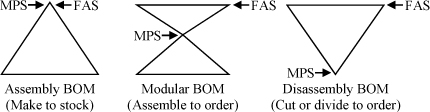
The Theory of Constraints (TOC) literature labels the processes for making these three BOMs as the A-plant, T-plant, and V-plant. See the VAT analysis entry for more detail.

The MPS is said to be “top management’s handle on the business,” because the MPS includes a very limited number of items. Therefore, the MPS process should focus on the narrow part of the BOM, which suggests that master scheduling should be done for end items for an assembly BOM, for major components for the modular BOM, and for raw materials for a disassembly BOM. Safety stock should be positioned at the same level as the MPS so that it is balanced between materials. In other words, a safety stock of zero units of item A and ten units of item B is of little value to protect against demand uncertainty if the end item BOM requires one unit of each. The Final Assembly Schedule (FAS) is a short-term schedule created in response to customer orders for the modular BOM. The push-pull boundary is between the items in the master schedule and in the FAS.

See assemble to order (ATO), Available-to-Promise (ATP), back scheduling, bill of material (BOM), Bill of Resources, Business Requirements Planning (BRP), Capacity Requirements Planning (CRP), chase strategy, Final Assembly Schedule (FAS), firm order, firm planned order, level strategy, Materials Requirements Planning (MRP), on-hand inventory, on-order inventory, production planning, push-pull boundary, Resource Requirements Planning (RRP), Rough Cut Capacity Planning (RCCP), safety leadtime, Sales & Operations Planning (S&OP), time fence, VAT analysis.

master schedule – The result of the master production scheduling process.

See Master Production Schedule (MPS).

master scheduler – The person responsible for creating the master production schedule.

See Master Production Schedule (MPS).

material delivery routes – See water spider.

Material Review Board (MRB) – A standing committee that determines the disposition of items of questionable quality.

materials handling – The receiving, unloading, moving, storing, and loading of goods, typically in a factory, warehouse, distribution center, or outside work or storage area.

Materials handling systems use four main categories of mechanical equipment: storage and handling equipment, engineered systems (e.g., conveyors, handling robots, AS/RS, AGV), industrial trucks (e.g., forklifts, stock chasers), and bulk material handling (e.g., conveyor belts, stackers, elevators, hoppers, diverters).

See forklift truck, inventory management, logistics, materials management, receiving, supply chain management.

materials management – The organizational unit and set of business practices that plans and controls the acquisition, creation, positioning, and movement of inventory through a system; sometimes called materials planning; nearly synonymous with logistics.

Materials management must balance the conflicting objectives of marketing and sales (e.g., have lots of inventory, never lose a sale, maintain a high service level) and finance (e.g., keep inventories low, minimize working capital, minimize carrying cost). Materials management often includes purchasing/procurement, manufacturing planning and control, distribution, transportation, inventory management, and quality.

If a firm has both logistics and materials management functions, the logistics function will focus primarily on transportation issues and the materials in warehouses and distribution centers and the materials management function will focus on procurement and the materials inside plants.

See carrying cost, inventory management, logistics, materials handling, purchasing, service level, supply chain management, Transportation Management System (TMS), warehouse, Warehouse Management System (WMS).

materials plan – See Materials Requirements Planning (MRP).

Materials Requirements Planning (MRP) – A comprehensive computer-based planning system for both factory and purchase orders; a major module within Enterprise Resources Planning Systems; also called Manufacturing Resources Planning.

MRP is an important module within Enterprise Requirements Planning (ERP) systems for most manufacturers. MRP was originally called Materials Requirements Planning and focused primarily on planning purchase orders for outside suppliers. MRP was then expanded to handle manufacturing orders sent to the shop floor, and some software vendors changed the name to Manufacturing Resources Planning.

MRP plans level by level down the bill of material (BOM). MRP begins by netting (subtracting) any on-hand and on-order inventory from the gross requirements. It then schedules backward from the due date using fixed planned leadtimes to determine order start dates. Lotsizing methods are then applied to determine order quantities. Lotsizes are often defined in terms of the number of days of net requirements. With MRP regeneration, a batch computer job updates all records in the database. With MRP net change generation, the system updates only the incremental changes.

MRP creates planned orders for both manufactured and purchased materials. The set of planned orders (that can be changed by MRP) and firm orders (that cannot be changed by MRP) is called the materials plan. Each order is defined by an order number, a part number, an order quantity, a start date, and a due date. MRP systems use the planned order start date to determine priorities for both shop orders and purchase orders. MRP is called a priority planning system rather than a scheduling system, because it backschedules from due dates using planned leadtimes that are calculated from the average queue times.

Nearly all MRP systems create detailed materials plans for an item using a Time Phased Order Point (TPOP) and fixed planned leadtimes. Contrary to what some textbooks claim, MRP systems rarely consider available capacity when creating a materials plan. Therefore, MRP systems are called infinite loading systems rather than finite loading systems. However, MRP systems can use Rough Cut Capacity Planning (RCCP) to check the Master Production Schedule (MPS) and Capacity Requirements Planning (CRP) to create load reports to check materials plans. These capacity checks can help managers identify situations when the plant load (planned hours) exceeds the capacity available. Advanced Planning and Scheduling (APS) systems are capable of creating detailed materials plans that take into account available capacity; unfortunately, these systems are hard to implement because of the need for accurate capacity, setup, and run time data.

See Advanced Planning and Scheduling (APS), allocated inventory, Available-to-Promise (ATP), bill of material (BOM), Business Requirements Planning (BRP), Capacity Requirements Planning (CRP), closed-loop MRP, dependent demand, Distribution Requirements Planning (DRP), effectivity date, Engineering Change Order (ECO), Enterprise Resources Planning (ERP), finite scheduling, firm order, forecast consumption, forward visibility, gross requirements, infinite loading, inventory management, kitting, low level code, Manufacturing Execution System (MES), manufacturing order, Master Production Schedule (MPS), net requirements, on-hand inventory, on-order inventory, pegging, phantom bill of material, planned order, production planning, purchase order (PO), purchasing, routing, time bucket, time fence, Time Phased Order Point (TPOP), where-used report.

matrix organization – An organizational structure where people from different units of an organization are assigned to work together under someone who is not their boss.

In a matrix organization, people work for one or more leaders who are not their bosses and who do not have primary input to their performance reviews. These people are “on loan” from their home departments. A matrix organization is usually (but not always) a temporary structure that exists for a short period of time. An example of a matrix organization is an architectural firm where people from each discipline (e.g., landscape architecture, heating, and cooling) temporarily report to a project manager for a design project.

See performance management system, project management.

maximum inventory – See periodic review system.

maximum stocking level – An SAP term for the target inventory.

See periodic review system.

MBNQA – See Malcolm Baldrige National Quality Award.

MCE (Manufacturing Cycle Effectiveness) – See value added ratio.

mean – The average value; also known as the arithmetic average.

The mean is the arithmetic average of a set of values and is a measure of the central tendency. For a sample of n values {x₁, x₂, ... x_n}, the sample mean is defined as . For the entire population of N values, the population mean is the expected value and is defined as . Greek letter μ is pronounced “mu.”

For a continuous distribution with density function f(x), the mean is the expected value 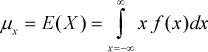, which is also known as the complete expectation and the first moment. The partial expectation, an important inventory theory concept, is defined as .

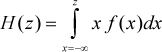The median is considered to be a better measure of central tendency than the mean when the data is likely to have outliners. The median is said to be an “error resistant” statistic.

See box plot, geometric mean, interpolated median, kurtosis, median, mode, partial expectation, skewness, trim, trimmed mean.

Mean Absolute Deviation (MAD) – A measure of the dispersion (variability) of a random variable; defined as the average absolute deviation from the mean.

The mathematical definition of the MAD for a random variable x_i with mean μ is . The standard deviation for a normally distributed random variable is theoretically exactly equal to (approximately 1.25MAD). This is true asymptotically³², but will rarely be true for any sample.

Brown (1967) implemented this approach widely at IBM, because early computers could not take square roots. However, by 1970, Brown argued that “MAD is no longer appropriate to the real world of computers. It never was the correct measure of dispersion” (Brown 1970, p. 148).

Other experts, such as Jacobs and Wagner (1989), argue that MAD is a still good approach, because absolute errors are less sensitive to outliers than the squared errors used in the variance and standard deviation. The MAD approach continues to be used in many major inventory management systems, including SAP.

In a forecasting context, the average error is often assumed to be zero (i.e., unbiased forecasts). In this context, . The MAD can be smoothed at the end of each period with the updating equation SMAD_t = σ|E_t| + (1 − α)SMAD_t−1. The smoothed MAD is sometimes called the smoothed absolute error or SAE.

See forecast bias, forecast error metrics, forecasting, Mean Absolute Percent Error (MAPE), mean squared error (MSE), Median Absolute Percent Error (MdAPE), outlier, Relative Absolute Error (RAE), robust, standard deviation, tracking signal, variance.

Mean Absolute Percent Deviation (MAPD) – See Mean Absolute Percent Error (MAPE).

Mean Absolute Percent Error (MAPE) – A commonly used (but flawed) measure of forecast accuracy that is the average of the absolute percent errors for each period; also called the Mean Absolute Percent Deviation (MAPD).

MAPE is defined mathematically as , where E_t is the forecast error in period t, D_t is the actual demand (or sales) in period t, and T is the number of observed values. Many firms multiply by 100 to rescale the MAPE as a percentage. Note that the MAPE is not the MAD divided by the average demand.

The MAPE has three significant problems. First, when the demand is small, the absolute percent error in a period (APE_t = |E_t|/D_t) can be quite large. For example, when the demand is 10 and the forecast is 100, the APE_t for that period is 90/10 = 9 (or 900%). These very large values can have an undue influence on the MAPE. Second, when the demand is zero in any period, the MAPE is undefined. Third, it is conceptually flawed. The MAPE is the average ratio, when it should be the ratio of the averages. In the opinion of many experts, the Mean Absolute Scaled Error (MASE) is a better metric than the MAPE because it avoids the above problems.

One way to try to fix the MAPE is to Winsorize (bound) the ratio in each period at 100%, which means that the MAPE is defined in the range [0%, 100%]. See the Winsorizing entry for details. However, in this author’s view, this “fix” only treats the symptoms of the problem.

The average MAPE can be misleading as an aggregate measure for a group of items with both low and high demand. For example, imagine a firm with two items. One item is very important with high demand, high unit cost, and low MAPE (e.g., 10%), and the other is a very unimportant item with low demand, low unit cost, and high MAPE (e.g., 90%). When these two MAPE values are averaged, the overall MAPE is 50%. However, this gives too much weight to the low-demand item and not enough to the important item. The weighted MAPE avoids this problem. The weighted average MAPE is defined as , where w_i is the importance weight for item i of N items. The annual cost of goods sold is the best weight to use in this equation.

Like many time series forecasting statistics, the MAPE can be smoothed with the updating equation SMAPE_t = α|E_t|/D_t + (1 − α)SMAPE_t−1. Be sure to Winsorize the APE_t when implementing this equation.

See demand filter, exponential smoothing, forecast bias, forecast error metrics, forecasting, Mean Absolute Deviation (MAD), Mean Absolute Scaled Error (MASE), mean squared error (MSE), Median Absolute Percent Error (MdAPE), Relative Absolute Error (RAE), Thiel’s U, tracking signal, Winsorizing.

Mean Absolute Scaled Error (MASE) – A forecast performance metric that is the ratio of the mean absolute deviation for a forecast scaled by (divided by) the mean absolute deviation for a random walk forecast.

Hyndman and Koehler (2006) proposed the MASE as a way to avoid many of the problems with the Mean Absolute Percent Error (MAPE) forecast performance metric. The MASE is the ratio of the mean absolute error for the forecast and the mean absolute error for the random walk forecast. Whereas the MAPE is the average of many ratios, the MASE is the ratio of two averages.

In the forecasting literature, the mean absolute error for the forecast error is called the Mean Absolute Deviation (MAD) and is defined as , where D_t is the actual demand and F_t is the forecast for period t. The random walk forecast for period t is the actual demand in the previous period (i.e., F_t = D_t–1); therefore, the Mean Absolute Deviation for the random walk is . This assumes a one-period-ahead forecast, but it can easily be modified for a k-period-ahead forecast. The MASE, therefore, is defined as MASE = MAD/MAD_RW.

The MASE will only have a divide-by-zero problem when the demand does not change over the entire horizon, but that is an unlikely situation. When MASE < 1, the forecasts are better than the random walk forecast; when MASE > 1, the forecasts are worse than the random walk forecast. A forecasting model with a MASE of 20% has a forecast error of 20% of the forecast error of the simplistic random walk forecast. A MASE of 95% is only slightly better than a simplistic random walk forecast.

The Mean Absolute Scaled Accuracy (MASA) is the companion accuracy measure for the MASE and is defined as 1 – MASE. MASA can be interpreted as the percent accuracy of the forecast relative to the accuracy of the random walk forecast. When MASA = 0, the forecasts are no better than the random walk forecast; when MASA < 0, the forecasts are worse than the random walk forecast; and when MASA = 60%, the average absolute forecast error is 40% of the average absolute forecast error for the random walk forecast. MASE and MASA are better measures of forecast accuracy than MAPE because they measure accuracy against an objective standard, which is the random walk forecast.

Hyndman and Koehler (2006, p. 13) assert that measures based on scaled measures (such as the MASE) “should become the standard approach in comparing forecast accuracy across series on different scales.” However, the MASE has two organizational challenges. First, it is not always easy to explain to managers. Second, when changing from MAPE to MASE, those responsible for forecasting will have to explain why the reported forecast accuracy decreases dramatically.

Dan Strike at 3M has suggests a very similar metric that uses a 12-month moving average as the scaling factor. This metric is even simpler than MASE to explain, but may be slightly harder to implement.

Thiel’s U₃ metric is the mean squared error scaled by the mean squared error for the random walk forecast. Therefore, it can be argued that the “new” MASE scaling concept is just an adaption of Thiel’s metric that uses the MAD rather than the mean squared error (MSE).

MASE can be implemented with simple moving averages or with exponential smoothing for both the numerator (the smoothed MAD) and the denominator (the smoothed MAD for a random walk forecast).

See forecast error metrics, Mean Absolute Percent Error (MAPE), Relative Absolute Error (RAE).

mean squared error (MSE) – The expected value of the square of the difference between an estimator and the parameter.

The MSE measures how far off an estimator is from what it is trying to estimate. In forecasting, the MSE is a measure of the forecast error that is the average of the squared forecast errors and is defined mathematically as , where E_t is the forecast error in period t and T is the number of observed values. The MSE is an estimate of the variance of the forecast error and is approximately equal to the variance when the forecast bias is close to zero. Like most time series statistics, the MSE can be smoothed with the updating equation . The root mean squared error (RMSE) is the square root of the MSE and is an estimate of the standard deviation of the forecast error. In fact, the RMSE will be equal to the standard deviation of the forecast error if the forecast is unbiased. Variances are additive, but standard deviations are not; therefore, RMSE is not normally smoothed.

See forecast bias, forecast error metrics, Mean Absolute Deviation (MAD), Mean Absolute Percent Error (MAPE), standard deviation, tracking signal, variance.

Mean Time Between Failure (MTBF) – A maintenance and reliability term for the average time that a component is expected to work without failing.

The MTBF is a good measure of product reliability. The MTBF is often modeled with the bathtub curve that has higher failure rates at the beginning and end of the product life cycle. The Mean Time For Failure (MTFF) is the average time to the first failure and is sometimes used for non-repairable products.

See availability, bathtub curve, maintenance, Mean Time to Repair (MTTR), New Product Development (NPD), reliability, Total Productive Maintenance (TPM).

Mean Time to Repair (MTTR) – A maintenance and reliability term for the average time required to fix something, such as a machine.

The MTTR is a measure of the complexity and cost of a repair job and a measure of the maintainability of a product (Schroeder 2007). The MTTR should not be used as the only performance measure for service techs because the best service techs are often assigned the most difficult repair jobs, which means they will have the highest MTTR. The same is true for doctors and other skilled professionals.

See availability, maintenance, Mean Time Between Failure (MTBF), New Product Development (NPD), serviceability, Total Productive Maintenance (TPM).

Measurement System Analysis (MSA) – An approach for verifying the accuracy and precision of a data measurement system using statistical analysis tools, such as Gauge R&R, attribute Gauge R&R, and the P/T ratio.

See Gauge, Gauge R&R, metrology.

MECE – The concept that an analysis should define issues and alternatives that are mutually exclusive and collectively exhaustive; pronounced “me-see.”

MECE thinking is widely used by strategy consulting firms, such as McKinsey, Bain, and BCG, to create both issue trees and decision trees (Rasiel 1998). In fact, the case interview method these firms use to screen applicants is designed to test MECE thinking.

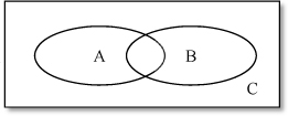
Mutually exclusive means that the ideas or alternatives are distinct and separate and do not overlap. Collectively exhaustive means that the ideas or alternatives cover all possibilities. The Venn diagram below shows two sets (A and B) that overlap and therefore are not mutually exclusive. The union of sets A, B, and C is collectively exhaustive because it covers all possibilities.

In most anlysies, it is far more important that issues be separable than MECE. For example, an outgoing shipment could be late because of mechanical problems with a truck or because the products were not ready to ship. These two events are not mutually exclusive, because they both could be true, but they can and should be studied separately.

See causal map, decision tree, issue tree, Minto Pyramid Principle, story board, Y-tree.

median – The middle value of a set of sorted values.

The median, like the mean, is a measure of the central tendency. The calculation of the median begins by sorting the values in a list. If the number of values is odd, the median is the middle value in the sorted list. If the number of values is even, the median is the average of the two middle values in the sorted list. For example, the median of {1, 2, , 9, 100} is 3, and the median of {1, 2, , 100, 200} is (3 + 9)/2 = 6.

The median is often a better measure of central tendency than the mean when the data is highly skewed. For example, consider the following selling prices for houses (in thousands): $175, $180, $200, $240, $241, $260, $800, and $2400. The mean is $562, but the median is only $240.5. In this case, the mean is “pulled up” by the two high prices.

Excel provides the function MEDIAN(range) for computing the median of a range of values.

Some people consider the interpolated median to be better than the median when many values are at the median and the data has a very limited number of possible values. For example, the interpolated median is often used for Likert survey questions on the 1-5 or 1-7 scale and also for grades in the U.S. that are translated from A, A-, B+, etc. to a 4.0 scale.

See box plot, forecast error metrics, interpolated median, mean, Median Absolute Percent Error (MdAPE), mode, skewness, trimmed mean.

Median Absolute Percent Error (MdAPE) – The middle value of all the percentage errors for a data set when the absolute values of the errors (negative signs are ignored) are ordered by size.

See forecast error metrics, Mean Absolute Deviation (MAD), Mean Absolute Percent Error (MAPE), median.

mergers and acquisitions (M&A) – The activity of one firm evaluating, buying, selling, or combining with another firm.

Whereas an acquisition is the purchase of one company by another, a merger is the combination of two companies to form a new company. In an acquisition, one firm will buy another to gain market share, create greater efficiency through economies of scale, or acquire new technologies or resources.

The goal for both mergers and acquisitions is to create shareholder value. The success of a merger or acquisition depends on whether this synergy is achieved from (1) growing revenues through synergies between products, markets, or product technologies or (2) economies of scale through headcount reduction, purchasing leverage, IT systems, HR, and other functional synergies. Unfortunately, planned synergies are not always realized, and in some cases revenues decline, morale sags, costs increase, and share prices drop.

See acquisition, antitrust laws, economy of scale.

Metcalfe’s Law – See network effect.

Methods Time Measurement (MTM) – See work measurement.

metrology – The science of measurement; closely related to Measurement System Analysis (MSA).

Metrology attempts to validate data obtained from test equipment and considers precision, accuracy, traceability, and reliability. Metrology, therefore, requires an analysis of the uncertainty of individual measurements to validate instrument accuracy. The dissemination of traceability to consumers (both internal and external) is often performed by a dedicated calibration laboratory with a recognized quality system.

Metrology has been an important topic in commerce since people started measuring length, time, and weight. For example, according to New Unger’s Bible Dictionary, the cubit was an important measure of length among the Hebrews (Exodus 25:10) and other ancient peoples. It was commonly measured as the length of the arm from the point of the elbow to the end of the middle finger, which is roughly 18 inches (45.72 cm).

The scientific revolution required a rational system of units and made it possible to apply science to measurement. Thus, metrology became a driver of the Industrial Revolution and was a critical precursor to systems of mass production. Modern metrology has roots in the French Revolution and is based on the concept of establishing units of measurement based on constants of nature, thus making measurement units widely available. For example, the meter is based on the dimensions of the Earth, and the kilogram is based on the mass of a cubic meter of water. The Système International d’Unités (International System of Units or SI) has gained worldwide acceptance as the standard for modern measurement. SI is maintained under the auspices of the Metre Convention and its institutions, the General Conference on Weights and Measures (CGPM), its executive branch, the International Committee for Weights and Measures (CIPM), and its technical institution, the International Bureau of Weights and Measures (BIPM). The U.S. agencies with this responsibility are the National Institute of Standards and Technology (NIST) and the American National Standards Institute (ANSI).

See gauge, Gauge R&R, lean sigma, Measurement System Analysis (MSA), reliability.

milestone – An important event in the timeline for a project, person, or organization.

A milestone event marks the completion of a major deliverable or the start of a new phase for a project. Therefore, milestones are good times to monitor progress with meetings or more formal “stage-gate” reviews that require key stakeholders to decide if the project should be allowed to continue to the next stage. In project scheduling, milestones are activities with zero duration.

See deliverables, project management, stage-gate process, stakeholder.

milk run – A vehicle route to pick up materials from multiple suppliers or to deliver supplies to multiple customers.

The traditional purchasing approach is for customers to send large orders to suppliers on an infrequent basis and for suppliers to ship orders to the customer via a common carrier. With a milk run, the customer sends its own truck to pick up small quantities from many local suppliers on a regular and frequent basis (e.g., once per week). Milk runs speed delivery and reduce inventory for the customer and level the load for the supplier, but at the expense of additional transactions for both parties. Milk runs are common in the automotive industry and are a commonly used lean practice. Hill and Vollmann (1986) developed an optimization model for milk runs.

See lean thinking, logistics, Vehicle Scheduling Problem (VSP).

min/max inventory system – See min-max inventory system.

mindmap – A diagram used to show the relationships between concepts, ideas, and words that are connected to a central concept or idea at one or more levels.

A mindmap is a graphical tool that can be used by an individual or a group to capture, refine, and share information about the relationships between concepts, ideas, words, tasks, or objects that are connected to a central concept or idea at one or more levels in a hierarchy. Mindmaps can be used to:

• Generate ideas

• Capture ideas

• Take course notes

• Provide structure to ideas

• Review and study ideas

• Visualize and clarify relationships

• Help plan meetings and projects

• Organize ideas for papers

• Create the storyboard for a presentation

• Stimulate creativity

• Create a shared understanding

• Create the agenda for a meeting

• Communicate ideas with others

• Teach concepts to others

• Document ideas

• Help make decisions

• Create a work breakdown structure

• Create a task list

• Prioritize activities

• Solve problems

A mindmap represents how one or more people think about a subject. The spatial organization on the paper (or screen) communicates the relationship between the nodes (ideas, concepts, objects, etc.) in the creator’s mind. Creating a mindmap helps the creators translate their thinking about a subject into more concrete ideas, which helps them clarify their own thinking and develop a shared understanding of the concepts. Once created, a mindmap is an excellent way to communicate concepts and relationships to others.

Methods – The concepts on a mindmap are drawn around the central idea. Subordinate concepts are then drawn as branches from those concepts. Buzan and Buzan (1996) recommend that the mindmaps should be drawn by hand using multiple colors, drawings, and photos. This makes the mindmap easier to remember, more personal, and more fun. They argue further that the mindmap should fit on one piece of paper, but allowed it to be a large piece of paper. Many powerful software packages are now available to create mindmaps, including Mind Manager (www.mindjet.com), Inspiration (www.inspiration.com), and many others.

Relationship to other mapping tools – A mindmap is similar to a causal map, except the links in a mindmap usually imply similarity rather than causality. A strategy map is a special type of causal map. A project network shows the time relationships between the nodes and therefore is not a mindmap. A bill of material (BOM) drawing and a work breakdown structure are similar to mindmaps in that they show relatedness and subordinated concepts.

Mindmap example – The example below was created by the author with Mindjet Mind Manager software to brainstorm both the work breakdown structure and the issue tree for a productivity improvement project. The symbol (+) indicates that additional nodes are currently hidden from view.

In conclusion, mindmaps are a powerful tool for visualizing, structuring, and communicating concepts related to a central idea. This author predicts that mindmapping software will become as popular as Microsoft’s process mapping tool (Microsoft Visio) and project management tool (Microsoft Project Manager).

Source: Professor Arthur V. Hill

See causal map, issue tree, process map, project network, strategy map, Work Breakdown Structure (WBS).

Minkowski distance metric – A generalized distance metric that can be used in logistics/transportation analysis, cluster analysis, and other graphical analysis tools.

If location i has coordinates (x_i, y_i), the Euclidean (straight-line) distance between points i and j is , which is based on the Pythagorean Theorem. The Manhattan square distance only considers travel along the x-axis and y-axis and is given by d_ij = |x_i − x_j | + |y_i − y_j|. The Minkowski distance generalizes these metrics and defines the distance as d_ij = (|x_i − x_j|^r + |y_i − y_j|^r)^1/r. The Minkowski distance metric is equal to the Euclidean distance when r = 2 and the Manhattan square distance when r = 1. Minkowski distance can be defined in multi-dimensional space. Consider item i with K attributes (dimensions) (i.e., x_i1, x_i2, ... , x_iK). The Minkowski distance between items i and j is then defined as .

The Chebyshev distance (also called the maximum metric and the L_∞ metric) sets the distance to the longest dimension (i.e., d_ij = max(|x_i−x_j|,|y_i−y_j|) and is equivalent to the Minkowski distance when r = ∞.

See cluster analysis, Manhattan square distance, Pythagorean Theorem.

min-max inventory system – An inventory control system that signals the need for a replenishment order to bring the inventory position up to the maximum inventory level (target inventory level) when the inventory position falls below the reorder point (the “min” or minimum level); known as the (s,S) system in the academic literature, labeled (R,T) in this book.

As with all reorder point systems, the reorder point can be determined using statistical analysis of the demand during leadtime distribution or with less mathematical methods. As with all order-up-to systems, the order quantity is the order-up-to level minus the current inventory position, which is defined as (on-hand + on-order – allocated – backorders).

A special case of a min-max system is the (S − 1, S) system, where orders are placed on a “one-for-one” basis. Every time one unit is consumed, another unit is ordered. This policy is most practical for low-demand items (e.g., service parts), high-value items (e.g., medical devices), or long leadtime items (e.g., aircraft engines).

See inventory management, order-up-to level, periodic review system, reorder point.

minor setup cost – See major setup cost, setup cost.

Minto Pyramid Principle – A structured approach to building a persuasive argument and presentation developed by Barbara Minto (1996), a former McKinsey consultant.

The Minto Pyramid Principle developed by Barbara Minto (1996) can improve almost any presentation or persuasive speech. Minto’s main idea is that arguments should be presented in a pyramid structure, starting with the fundamental question (or hypothesis) at the top and cascading down the pyramid, with arguments at one level supported by arguments at the next level down. At each level, the author asks, “How can I support this argument?” and “How do I know that this is true?” The presentation covers all the arguments at one level, and then moves down to the next level to further develop the argument.

For example, a firm is considering moving manufacturing operations to China. (See the figure below.) At the top of the pyramid is the hypothesis, “We should move part of our manufacturing to China.”

Example of the Minto Pyramid Principle

Source: Professor Arthur V. Hill

From this, the team doing the analysis and making the presentation asks, “Why is it a good idea to move to China?” The answer comes at the next level with three answers: (1) We will have lower labor cost in China, (2) we can better serve our customers in Asia, and (3) locating in China will eventually open new markets for the company’s products in China. The team then asks “Why?” for each of these three items and breaks these out in more detail at the next level. The “enable us to lower our direct labor cost” argument is fully developed before the “better able to serve our customers in Asia” is started.

Minto recommends that the presentation start with an opening statement of the thesis, which consists of a factual summary of the current situation, a complicating factor or uncertainty that the audience cares about, and the explicit or implied question that this factor or uncertainty raises in the audience’s mind and that the presenter’s thesis answers. The closing consists of a restatement of the main thesis, the key supporting arguments (usually the second row of the pyramid), and finally an action plan.

See hypothesis, inductive reasoning, issue tree, MECE, story board.

mission statement – A short statement of an organization’s purpose and aspirations, intended to provide direction and motivation.

Most organizations have a vision statement or mission statement that is intended to define their purpose and raison d’être³³. However, for many organizations, creating a vision or mission statement is a waste of time. Vision and mission statements are published in the annual report and displayed prominently on the walls, but they are understood by few, remembered by none, and have almost no impact on anyone’s thinking or behavior. Yet this does not have to be the case. Vision and mission statements can be powerful tools for aligning and energizing an entire organization.

Although scholars do not universally agree on the difference between vision and mission statements, most view the vision statement as the more strategic longer-term view and argue that the mission should be derived from the vision. A vision statement should be a short, succinct, and inspiring statement of what the organization intends to become at some point in the future. It is the mental image that describes the organization’s aspirations for the future without specifying the means to achieve those aspirations. The table below presents examples of vision statements that have worked and others that probably would not have worked.

Of course, having a vision, mission, goals, and objectives is not enough. Organizations need to further define competitive strategies and projects to achieve them. A competitive strategy is a plan of action to achieve a competitive advantage. Projects are a means of implementing strategies. Projects require goals and objectives, but also require a project charter, a team, and a schedule. Strategies and projects should be driven by the organization’s vision and mission. The hoshin planning, Y-tree, and strategy mapping entries present important concepts on how to translate a strategy into projects and accountability.

The mission statement translates the vision into more concrete and detailed terms. Many organizations also have values statementS dealing with integrity, concern for people, concern for the environment, etc., where the values statement defines constraints and guides all other activities. Of course, the leadership must model the values. Enron’s motto was “Respect, Integrity, Communication and Excellence” and its vision and value statement declared “We treat others as we would like to be treated ourselves ... We do not tolerate abusive or disrespectful treatment. Ruthlessness, callousness and arrogance don’t belong here” (source: http://wiki.answers.com, May 8, 2011). However, Enron’s leadership obviously did not live up to it.

Goals and objectives are a means of implementing a vision and mission. Although used interchangeably by many, most people define goals as longer term and less tangible than objectives. The table below on the left shows the Kaplan and Norton model (2004), which starts with the mission and then follows with values and vision. This hierarchy puts mission ahead of values and vision. The table below on the right is a comprehensive hierarchy developed by this author that synthesizes many models.

In conclusion, vision and mission statements can be powerful tools to define the organization’s desired end state and to energize the organization to make the vision and mission a reality. To be successful, these statements need to be clear, succinct, passionate, shared, and lived out by the organization’s leaders. They should be supported by a strong set of values that are also lived out by the leadership. Lastly, the vision and mission need to be supported by focused strategies, which are implemented through people and projects aligned with the strategies and mission.

See Balanced Scorecard, forming-storming-norming-performing model, hoshin planning, SMART goals, strategy map, true north, Y-tree.

mistake proofing – See error proofing.

mix flexibility – See flexibility.

mixed integer programming (MIP) – A type of linear programming where some decision variables are restricted to integer values and some are continuous; also called mixed integer linear programming.

See integer programming (IP), linear programming (LP), operations research (OR).

mixed model assembly – The practice of assembling multiple products in small batches in a single process.

For example, a firm assembled two products (A and B) on one assembly line and used large batches to reduce changeover time with sequence AAAAAAAAAAAAAAABBBBBBBBBBBBBB. However, the firm was able to reduce changeover time and cost, which enabled it to economically implement mixed model assembly with sequence ABABABABABABABABABABABABABABA.

The advantages of mixed model assembly over the large batch assembly are that it (1) reduces inventory, (2) improves service levels, (3) smoothes the production rate, and (4) enables early detection of defects. Its primary disadvantage is that it requires frequent changeovers, which can add complexity and cost.

See assembly line, early detection, facility layout, heijunka, manufacturing processes, service level, setup time reduction methods.

mizusumashi – See water spider.

mode – (1) In a statistics context: The most common value in a set of values. (2) In a transportation context: The method of transportation for cargo or people (e.g., rail, road, water, or air).

In the statistics context, the mode is a measure of central tendency. For a discrete distribution, the mode is the value where the probability mass function is at its maximum value. In other words, the mode is the value that has the highest probability. For a continuous probability distribution, the mode is the value where the density function is at its maximum value. However, the modal value may not be unique. For symmetrical distributions, such as the normal distribution, the mean, median, and mode are identical.

In the transportation context, the mode is a type of carrier (e.g., rail, road, water, air). Water transport can be further broken into barge, boat, ship, ferry, or sailboat and can be on a sea, ocean, lake, canal, or river. Intermodal shipments use two or more modes to move from origin to destination.

See intermodal shipments, logistics, mean, median, multi-modal shipments, skewness.

modular design (modularity) – Organizing a complex system as a set of distinct components that can be developed independently and then “plugged” together.

The effectiveness of the modular design depends on the manner in which systems are divided into components and the mechanisms used to plug components together. Modularity is a general systems concept and is a continuum describing the degree to which a system’s components can be separated and recombined. It refers to the tightness of coupling between components and the degree to which the “rules” of the system architecture enable (or prohibit) the mixing and matching of components. Because all systems are characterized by some degree of coupling between components and very few systems have components that are completely inseparable and cannot be recombined, almost all systems are modular to some degree (Schilling 2000).

See agile manufacturing, commonality, interoperability, mass customization.

modularity – See modular design.

mold – A hollow cavity used to make products in a desired shape.

See foundry, manufacturing processes, tooling.

moment of truth – A critical or decisive time on which much depends; in the service quality context, an event that exposes a firm’s authenticity to its customers or employees.

A moment of truth is an opportunity for the firm’s customers (or employees) to find out the truth about the firm’s character. In other words, it is a time for customers or employees to find out “who we really are.” This is a chance for employees (or bosses) to show the customers (or employees) that they really do care about them and to ask customers (or employees) for feedback on how products and services might be improved. These are special moments and should be managed carefully.

When creating a process map, it is important to highlight the process steps that “touch” the customer. A careful analysis of a typical service process often uncovers many more moments of truth than management truly appreciates. Such moments might include a customer phone call regarding a billing problem, a billing statement, and an impression from an advertisement.

People tend to remember their first experience (primacy) and last experience (recency) with a service provider. It is important, therefore, to manage these important moments of truth with great care.

The book Authenticity (Pine & Gillmore 2007) argues that in a world increasingly filled with deliberately staged experiences and manipulative business practices (e.g., frequent flyer programs), consumers often make buying decisions based on their perception of the honesty, integrity, and transparency of a service provider. This definition of authenticity is closely related to the concept of a moment of truth.

See primacy effect, service blueprinting, service management, service quality.

Monte Carlo simulation – See simulation.

Moore’s Law – A prediction made by Intel cofounder Dr. Gordon E. Moore in 1965 stating that the number of components on an integrated circuit will double every 12 months (or 18 months or 24 months).

In 1975, Moore revised his 12 months to 24 months. Other people have revised the law to the widely quoted number of 18 months, which is an average of the 12 and 24 months. Moore’s Law is really not a “law.” It is simply an empirical observation that the number of components on a circuit was growing at an exponential rate.

Moore was not the first person to make this kind of observation. In 1751, Benjamin Franklin noted in his essay “Observations Concerning the Increase of Mankind, Peopling of Countries, etc.,” that “This million doubling, suppose but once in 25 years, will, in another century, be more than the people of England, and the greatest number of Englishmen will be on this side of the water.”

Moore’s Law is an exponential growth model of a continuous variable that can be applied to many fast-growth contexts, such as millions of instructions per second (MIPS) for the fastest computer, the number of Internet users, and the mosquito population in Minnesota.

The mathematical model for exponential growth is identical to the exponential decay half-life “time-based learning” model, and both use the form y(t) = ae^bt. Unlike the learning curve model that has discrete time periods, the exponential growth (or decay) model is expressed in continuous time. Whereas the performance variable for exponential growth doubles every h time periods, the performance variable for the half-life curve “halves” every h time periods. The constants for both models are a = y(0), b = ln(2)/h, and h = ln(2)/b, but the signs for b and h are opposite those of the half-life model.

See green manufacturing, half-life curve, learning curve, learning organization.

moving average – An average over the last n periods often used as a short-term forecast; also called a rolling average, rolling mean, or running average.

The moving average can be used to make forecasts based on the most recent data. It can also be used to smooth data for graphing purposes.

An n-period moving average is the arithmetic average of the last n periods of a time series. For a time series (d₁, d₂, ... , d_T), the moving average is . In other words, a moving average is a weighted average with equal weights that sum to one for the last n periods and zero weights for all values more than n periods old.

An exponentially smoothed average (sometimes called an exponential moving average) is like a moving average in that it is also a weighted average and an average of the recent data for a time series. Whereas a moving average uses equal weights for the last n periods and zero weights for all values more than n periods old, an exponentially smoothed average uses weights that decline geometrically with the age of the data. When the demand is stationary, an n-period moving average can be proven to have the same expected value as a simple exponential smoothed average with smoothing constant α = 2 / (n + 1).

See Box-Jenkins forecasting, centered moving average, exponential smoothing, forecasting, time series forecasting, weighted average.

MPS – See Master Production Schedule.

MRB – See Material Review Board.

MRO – See Maintenance-Repair-Operations (MRO).

MRP – See Materials Requirements Planning (MRP).

MTBF – See Mean Time Between Failure (MTBF).

MTM (Methods Time Measurement) – See work measurement.

MTO – See make to order (MTO).

MTS – See make to stock (MTS).

MTTR – See Mean Time to Repair (MTTR).

muda – A Japanese word for waste used to describe any activity that does not add value.                      

In conversational Japanese, “muda” means useless, futile, or waste. In popular lean manufacturing terminology, muda is any type of waste. All eight of the “8 wastes” are examples of muda: over-production, waiting, conveyance, processing, inventory, motion, correction, and wasted human potential.

According to the Lean Enterprise Institute, “muda,” “mura,” and “muri” are three Japanese terms often used together in the Toyota Production System to describe wasteful practices that should be eliminated.

• Muda (Non-value-added) – Any activity that consumes resources without creating value for the customer.

• Mura (Imbalance) – Unevenness in an operation; for example, an uneven work pace in an operation causing operators to hurry and then wait.

• Muri (Overload) – Overburdening or causing strain on equipment or operators.

See 8 wastes, error proofing, lean thinking, Toyota Production System (TPS).

multi-modal shipments – Moving goods using two or more modes of transportation; also called multi-modal transport.

An example is a container picked up from the shipper by truck, loaded onto the rail, shipped by rail to a port, and then loaded onto a vessel. Multi-modal shipments help optimize supply chain efficiency, but can make tracking difficult because of the need for coordination between the modes.

See intermodal shipments, logistics, mode, shipping container.

multiple source – See single source.

multiple-machine handling – The practice of assigning workers to operate more than one machine at a time.

This is a common Japanese manufacturing practice that is made possible by the application of jidoka and error proofing principles. Chaku-Chaku is an application of this principle.

See Chaku-Chaku, error proofing, jidoka.

multiplication principle – Investing strategically in process improvements that can be “multiplied” (i.e., used) over many transactions.

Love (1979) challenged people to invest time and money to improve processes, particularly when a one-time investment can be multiplied over many transactions. Good examples include creating checklists, writing standard operating procedures, reducing setup time, automating a process, creating a standard legal paragraph, and applying 5S. The multiplication principle suggests that organizations should focus their process improvement efforts on those repetitive activities that cost the most.

See 5S, addition principle, automation, checklist, human resources, job design, lean thinking, setup time reduction methods, subtraction principle.

mura – See muda.

muri – See muda.

Murphy’s Law – A humorous and pessimistic popular adage often stated as, “If anything can go wrong, it will” or “Anything that can go wrong will go wrong.”

Murphy’s Law is similar to the Second Law of Thermodynamics (sometimes called the law of entropy), which asserts that all systems move to the highest state of disorder (the lowest possible state of energy) and tend to stay there unless energy is supplied to restore them. O’Toole’s commentary on Murphy’s Law is “Murphy was an optimist.” The website http://userpage.chemie.fu-berlin.de/diverse/murphy/murphy2.html (April 1, 2011) offers many similar types of “laws.”

See error proofing, Parkinson’s Laws, project management.

N

NAFTA – See North American Free Trade Agreement (NAFTA).

nanotechnology – The study of the control of materials on an atomic or molecular scale; also called nanotech.

“Nano” means a billionth. A nanometer is one-billionth of a meter. Nanotechnology generally deals with structures of the size of 100 nanometers or smaller.

See disruptive technology.

NAPM (National Association of Purchasing Management) – See Institute for Supply Management (ISM).

National Association of Purchasing Management (NAPM) – See Institute for Supply Management (ISM).

NC machine – See Numerically Controlled (NC) machine.

near miss – See adverse event.

nearshoring – The practice of moving work to a neighboring country; also called near shore outsourcing.

U.S. firms nearshore to Canada and Mexico as well to Central and South America and the Caribbean. Firms in Western Europe nearshore to central and Eastern Europe. Whereas offshoring means to move work to any other country (possibly across an ocean), nearshoring means to move work to another country in the same region. The term “nearshoring” often implies outsourcing to another firm, but technically, it is possible for a firm to nearshore to a plant owned by the firm in another nearby country. The advantages of keeping the work in a nearby region can include better communication (particularly if the countries share the same language), better cultural understanding (leading to trust), less travel distance (leading to reduced cost and more frequent visits and tighter controls), and fewer time zones (leading to easier and more frequent communication).

See offshoring, outsourcing, sourcing.

necessary waste – See 8 wastes.

negative binomial distribution – A discrete probability distribution that counts the number of successes (or failures) in a sequence of independent Bernoulli trials (each with probability of success p) before the r-th failure (or success); also known as the Pascal distribution, Pólya distribution, and gamma-Poisson distribution.

The negative binomial is the discrete analog to the gamma distribution and therefore can take on many shapes. Like the gamma and Poisson, the negative binomial is only defined for non-negative values (i.e., x0).

The Poisson distribution is the most commonly used discrete probability distribution in inventory theory, but has only one parameter and is only appropriate when the mean and variance are approximately equal. The negative binomial distribution is a good alternative to the Poisson when the data is “dispersed” (i.e., σ² > μ).

Parameters: r > 0 is the number of failures and p is the probability of success on each experiment.

Probability mass and cumulative distribution functions: , where x is a non-negative integer, p is a probability, and r is an integer for the Pascal version but can be any real positive number for the Pólya version. For the Pólya version with non-integer r, , where Γ(.) is the gamma function. Note that this distribution can be parameterized in many ways, so care must be taken to not confuse them. The CDF has no closed form, but can be written as F(x) = I(p;r,x + 1), where I(p;r,x + 1) is the regularized beta function. (See the beta function entry for more information.)

Statistics: Range x{0, 1, 2, ... }, mean μ = r(1 − p)/p, variance σ² = rp/(1 − p)² = μ/(1 − p), and mode (r − 1)p/(1 − p) if r > 1; 0 otherwise.

Graph: The graph below is the negative binomial probability mass function with r = 5 trials of a fair coin (p = 0.5).

Parameter estimation: The method of moments parameters are p = 1 − μ/σ² and r = μ(1 − p)/p. Many authors recommend a Maximum Likelihood Estimator (MLE) approach over the method of moments estimators.

Excel: In Excel, the probability mass function is NEGBINOMDIST(x, r, p) and is interpreted as the probability of x failures before the r-th success when the probability of a success on any one trial is p.

Excel simulation: An Excel simulation can use the inverse transform method to generate negative binomial random variates using a direct search for the inverse cumulative CDF function.

Relationships to other distributions: The geometric distribution is a special case of the negative binomial distribution for r = 1. The sum of r independent geometric(p) random variables is a negative binomial (r, p) random variable. The sum of n negative binomial random variables with parameters (r_i, p) is a negative binomial with parameters (Σr_i, p). The negative binomial converges to the Poisson as r approaches infinity, p approaches 1, and μ is held constant. The Pascal distribution (after Blaise Pascal) and Pólya distribution (after George Pólya) are special cases of the negative binomial. The convention among statisticians and engineers is to use the negative binomial (or Pascal) with an integer-valued r and use Pólya with a real-valued r. The Pólya distribution more accurately models occurrences of “contagious” discrete events, such as tornado outbreaks, than does the Poisson distribution.

See Bernoulli distribution, beta function, gamma distribution, Poisson distribution, probability distribution, probability mass function.

negative exponential distribution – See exponential distribution.

net change MRP – See Materials Requirements Planning (MRP).

Net Present Value (NPV) – The future stream of benefits and costs converted into equivalent values today.

The NPV is calculated by assigning monetary values to benefits and costs, discounting future benefits and costs using an appropriate discount rate, and subtracting the sum total of discounted costs from the sum total of discounted benefits. Mathematically, NPV is defined as , where t is the time period, n is the number of periods, r is the discount rate, C_t is the net cash flow in period t, and C₀ is the initial cash outlay.

See financial performance metrics.

Net Promoter Score (NPS) – A simple but useful loyalty metric based on customers’ willingness to recommend.

The Net Promoter Score (NPS) is a relatively new loyalty metric developed by Frederick Reichheld (2003). It is derived from the “willingness to recommend metric,” which is a survey instrument with the single item (question), “How likely is it that you would recommend us to a friend or colleague?”

Customers are asked to respond using a 0-10 Likert rating scale with 0 anchored on the extreme negative end and 10 on the extreme positive end. Customers are then divided into three categories: (1) promoters (9 or 10) are loyal enthusiasts who keep buying from a company and urge their friends to do the same; (2) passives (7 or 8) are satisfied but unenthusiastic customers who can be easily wooed by the competition; and (3) detractors (0 to 6) are unhappy customers. The NPS is the percentage of promoters minus the percentage of detractors. Reichheld (2003) compared the NPS to a financial net worth that takes the assets minus the liabilities, where the assets are the promoters and the liabilities are the detractors.

Reichheld (2003) claims that the NPS is the single best predictor of customer loyalty. He argues that the NPS is highly correlated with growth rates and that it is the single most reliable indicator of a company’s ability to grow. The consulting firm Satmetrix offered a short white paper on this subject found at www.satmetrix.com/pdfs/NetPromoterWPfinal.pdf, May 16, 2011.

Dixon, Freeman, and Toman (2010) claim that the Customer Effort Score (CES) is more predictive of customer loyalty in a call center context than either the NPS or customer satisfaction.

Hill, Hays, and Naveh (2000) develop a concept similar to the NPS based on an economic model showing that loyalty is related to the ratio (not the difference) of satisfied and dissatisfied customers; i.e., Π_s/(1 − Π_s), where Π_s is the percent satisfied. This suggests that loyalty might be a function of the ratio Π_p/Π_d, where Π_p is the percent promoters and Π_d the percent detractors, rather than the difference Π_p − Π_d. This concept has not yet been tested empirically.

See Customer Effort Score (CES), operations performance metrics, service management, service quality.

net requirements – The number of units still needed to satisfy the materials plan in a Materials Requirements Planning (MRP) system.

In the MRP planning process, the net requirement is calculated as the gross requirements (units needed by higher-level items) plus allocations (units already promised to an order), less on-hand inventory (units that are available now), less open orders (scheduled receipts that will soon be available), less safety stock (desired number of units on-hand at all times).

See Materials Requirements Planning (MRP), open order.

net weight – (1) In a packaging context: The weight of a product without packaging. (2) In a shipping/logistics context: The weight of a vehicle without its fuel, cargo, personnel, pallets, containers, or straps.

See gross weight, logistics, tare weight.

network effect – An economics term that describes a situation where the value of a product or service increases with the number of adopters, thereby encouraging an increasing number of adopters; also called a network externality.

The network effect can be illustrated with cell phones. If the world had only one cell phone that used a particular communication technology, it would be of no value. However, this cell phone would become much more valuable if two of them existed, even more valuable if four of them existed, and far more valuable if nearly everyone had one.

Economists call this a network externality because when new consumers join the network, they have a beneficial external impact on consumers already in the network. The network effect produces a self-reinforcing cycle, with more buyers attracting more buyers.

Metcalfe’s Law states, “The value of a telecommunications network is proportional to the square of the number of users of the system (n²)” (Shapiro & Varian 1999). Metcalfe’s Law explains many of the network effects of communication technologies and networks, such as the Internet, social networking, and Wikipedia. It is related to the fact that the number of unique connections in a network with n nodes is n(n − 1)/2. Briscoe, Odlyzko, and Tilly (2006) argues that Metcalfe’s Law is wrong and proposes n log(n) as an alternative growth model. With both models, the value of the network grows faster than a linear growth rate. If cost grows linearly with n and value grows faster than linear, the value will eventually exceed the cost.

The network effect is enabled by the interoperability of the network. The network effect is often the result of word-of-mouth testimonials. In other words, people may adopt a service because “everyone” uses it. Over time, positive network effects can create a “bandwagon effect” as the network becomes more valuable. This is related to the Bass Model.

The expression network effect nearly always refers to positive network externalities, as in the case of the telephone. Negative network externalities can also occur where more adopters make a product less valuable. This is sometimes referred to as “congestion,” as in automobile congestion on the road.

With economy of scale, the supply side of a business becomes more efficient as it grows. With the network effect, the demand side of a business becomes more valuable as it grows. The network effect, therefore, is essentially a demand side economy of scale.

See Bass Model, economy of scale, interoperability.

network optimization – An operations research term for an efficient approach for modeling and solving a class of linear programming problems.

Many problems can be modeled as a network optimization problem, including the assignment problem, the transportation problem, and the transshipment problem. Most network optimization problems can be represented by a set of notes with arrows connecting them (a directed graph). The user must define the minimum flow, maximum flow, and cost per unit flow that can pass along each arc in the network. The fundamental rule is conservation of flow, which states simply that the flow coming into a node must equal the flow going out of a node. Only one type of commodity (product) can be modeled. More general methods, such as linear and integer programming, can handle multiple commodity flows.

The Ford and Fulkerson “out-of-kilter” algorithm is the most famous approach for solving this problem, but primal network algorithms are much more efficient. Several variants of the Ford and Fulkerson algorithm are available in the public domain and are efficient enough to handle many practical problems.

See algorithm, assignment problem, linear programming (LP), operations research (OR), optimization, transportation problem, transshipment problem.

neural network – A computer program that can “learn” over time; often called an “artificial neural network.”

A neural network is a program that creates a computer network designed to function in a similar way to natural neural structures, such as a human brain. They can be used to model complex relationships between inputs and outputs or to find patterns in data. Neural networks are sometimes used in data mining applications to try to find relationships between inputs and outputs.

For example, neural networks might be helpful in identifying which customers have high credit risk based on history with other customers. In another example, a neural network approach was used at the University of Minnesota to try to identify how much of a particular polymer was found in a microscopic digitized photo. The program was “trained” by hundreds of photos that had many variables describing each pixel in the photo. Over time, the neural net program was able to develop a simple set of decision rules that could be used to correctly classify future pixels most of the time.

See Artificial Intelligence (AI), data mining.

never event – See sentinel event.

New Product Development (NPD) – The process of generating new product and service concepts, creating designs, and bringing new products and services to market; also called product development.

The NPD process is often divided into three steps:

The fuzzy front end – The activities that generate and select concepts to be started into product development. Organizations should only start concepts that have a high probability of financial success.

New product development – The process of translating product concepts into specific designs that can be manufactured and brought to market.

Commercialization – The process of managing a new product through pilot production, production ramp-up, and product launch into the channels of distribution.

One of the key issues for NPD is forming the NPD project team. The following four tables compare the NPD team structure for four types of organizations: functional, lightweight, heavyweight, and autonomous. A good reference on this subject is Clark and Wheelwright (1992).

Product Development and Management Association (PDMA) and the Product Development Institute (PDI) are two of the leading professional societies for NPD professionals in North America.

The Toyota approach to NPD appears to be quite different from that used in Western Europe and North America. Morgan and Liker (2006) provided a good overview of the Toyota NPD process.

See absorptive capacity, adoption curve, Analytic Hierarchy Process (AHP), autonomous workgroup, breadboard, clockspeed, commercialization, Computer Aided Design (CAD), concurrent engineering, configuration management, Design for Six Sigma (DFSS), disruptive technology, Early Supplier Involvement (ESI), Fagan Defect-Free Process, flexibility, fuzzy front end, High Performance Work Systems (HPWS), ideation, Integrated Product Development (IPD), job design, Kano Analysis, lean design, line extension, Mean Time Between Failure (MTBF), Mean Time to Repair (MTTR), phase review, planned obsolescence, platform strategy, postponement, process design, Product Data Management (PDM), project charter, project management, prototype, Pugh Matrix, Quality Function Deployment (QFD), reliability, reverse engineering, scrum, serviceability, simultaneous engineering, stage-gate process, technology road map, time to market, time to volume, TRIZ, voice of the customer (VOC), waterfall scheduling.

new product flexibility – See flexibility.

newsvendor model – A mathematical model that solves the newsvendor problem, which is an important problem where the decision maker must decide how much to purchase given the probability distribution of demand, the cost of under-buying one unit, and the cost of over-buying one unit; formerly called the newsboy model or the newsboy problem.

The newsvendor problem appears in many business contexts, such as buying for a one-time selling season, making a final production run, setting safety stocks, setting target inventory levels, and making capacity decisions. These contexts all have the same problem structure: a single policy parameter, such as the order quantity, the presence of random demand, and known unit overage and unit underage costs.

The newsvendor model is fundamental to solving many important operations problems. The intuition obtained from the model can also be helpful. Explicitly defining the over-buying and under-buying cost and calculating the critical ratio can lead managers and analysts to better decisions.

The optimal order quantity is the demand associated with the critical ratio (also called the critical fractile), which is R = c_u/(c_u + c_o), where c_u is the cost of having one unit less than the realized demand, and c_o is the unit cost of having one unit more than the realized demand. In the simplest retail environment, c_u is price minus unit cost (the gross margin), and c_o is unit cost minus salvage value. The optimal order quantity is Q* = F⁻¹(R), where F⁻¹(R) is the inverse of the cumulative distribution function evaluated at the critical ratio.

For example, a grocery store owner needs to buy newspapers every Monday. If the owner buys one newspaper more than the demand, the store loses the cost of the newspaper (c_o = unit cost = $0.10). If the owner buys one newspaper less than the demand, the store loses the margin on the newspaper (c_u = unit price − unit cost = $0.50 − $0.10 = $0.40). The critical ratio, therefore, is R = c_u/(c_u + c_o) = 0.4/(0.4 + 0.1) = 90%, and the optimal order quantity is at the 90th percentile of the cumulative demand distribution (CDF).

For the normal distribution, the Excel function for the optimal order quantity is NORMINV(critical ratio, mean, standard deviation). For example, if we have a newsvendor problem with normally distributed demand with a mean of 4 units, a standard deviation of 1 unit, and costs c_o = $100 and c_u = $1000, the critical ratio is R = 0.91, and the optimal order quantity is Q* = NORMINV(0.91, 4, 1) = 5.34 units.

See anchoring, bathtub curve, capacity, fractile, Poisson distribution, purchasing, safety stock, seasonality, slow moving inventory, stockout, triangular distribution.

newsvendor problem – See newsvendor model.

Newton’s method – An important numerical method for “finding the roots” of the function; also known as the Newton-Raphson iteration.

The roots of a function f(x) are the x values where f(x) = 0. Newton’s method uses the Newton step x_k+1 = x_k − f(x_k)/f′(x_k) to find a better x value with each iteration. For “well-behaved” functions, Newton’s method usually converges very quickly, usually within five to ten steps. However, the choice of the starting point x₀ is important to the speed of convergence. The method will converge when df / dx and d² f / dx² do not change signs between x₀ and the root of f(x) = 0. Cheney and Kincaid (1994) identified three possible situations where Newton’s procedure will not converge. These are the runaway problem, the flat spot problem, and the cycle problem.

See linear programming (LP), operations research (OR).

NGT – See Nominal Group Technique (NGT).

no fault receiving – A way of inventory accounting used in retailing where store employees are only required to “count boxes” and put the items away; employees are not required to account for the item count in each box.

See receiving.

nominal capacity – See capacity.

Nominal Group Technique (NGT) – A planning tool that helps a group organize and prioritize issues and gain buy-in through the process.

Originally developed as an organizational planning technique by Delbecq, Van de Ven, and Gustafson in 1971, the nominal group technique can be used as an alternative to both the focus group and the Delphi techniques. It presents more structure than the focus group, but still takes advantage of the synergy created by group participants. The NGT helps build agreement on the issues in the process. This author uses the following approach for facilitating NGT brainstorming sessions:

1. Prepare – The leader in the organization should define the main question, find a skilled facilitator, select a group of participants, instruct the participants to come prepared to address the main question, arrange for a room with some empty walls, get marking pens (to make it hard for people to write too small) and Post-it Notes (at least 20 per participant). The 3M lined 4×6 Super-Sticky Post-it Notes work well.

2. Kickoff – The facilitator should open the meeting by clearly defining the main question (e.g., “How can we reduce waiting times for our customers?”) and the scope of the discussion (e.g., “Our scope will not include information system issues.”). The facilitator should this question on the whiteboard or easel and then ask the participants if they have any questions about the main question or scope before beginning.

3. Generate – Participants should then spend about five to ten minutes thinking quietly and creatively about the main question and generating a number of ideas to address the question. (In this author’s experience, very few workgroups are disciplined enough to prepare their notes before the meeting.) Each participant should write each idea on a separate Post-it Note, with a one to five word title in very large (one-inch high) letters on the top half of the note. Notes must be readable from the other side of the room. The facilitator should instruct participants to put their markers down when done. The facilitator should move on to the next step when about three quarters of the participants have their markers down.

4. Share – Each participant is asked to share just one note for each round. The facilitator should add each note to the wall, trying to group them logically. For smaller groups, it works well to have everyone stand at the wall during this process. Discussion is not allowed during this time, except to ask short clarification questions. Participants should share their duplicate notes first and then add one new idea (note) to the wall. Participants should feel free to pass and then jump back in if they think of other contributions. The process should continue around the room until all notes are on the wall.

5. Group – The facilitator should ask for two or three volunteers to come to the wall and organize the notes into groups while other participants take a short break.

6. Regroup – When people return from break, they should come to the wall and study the groups. They can move a note from one group to another, combine two or more groups, add a new group, add new notes, and make copies of notes that belong to more than one group.

7. Arrange – With help from the participants, the facilitator should arrange groups in logical order on the wall (e.g., time order or in some sort of hierarchy). Some groups might become subgroups of larger groups. This process may require additional title notes.

8. Vote – Each participant should vote on the top three groups he or she believes is worthy of further discussion and action. (The facilitator should only allow two votes per person if the number of groups is less than four.)

9. Assign – Organizing the ideas into groups and prioritizing them is usually just the starting point. It is now necessary to determine the next steps. It is important to decide who has ownership for a particular issue or solution and to clearly define the next steps for that person. In some cases, it is also a good idea to begin to create a formal project to address the top issues.

Advantages of the NGT process over typical brainstorming include:

• Shows respect for all participants and their ideas.

• Does not allow “high-verbal” or “high-control” participants to dominate the discussion.

• Collects many ideas from the participants along with detailed documentation of these ideas.

• Efficiently creates a set of notes to document the ideas using the participants’ own words.

• Very quickly and efficiently groups and prioritizes ideas.

• Results in good solutions.

• Creates a shared understanding of the problems and the solutions.

• Builds a strong sense of ownership of the results.

See affinity diagram, brainstorming, causal map, focus group, ideation, impact wheel, issue log, Kepner-Tregoe Model, KJ Method, parking lot, Root Cause Analysis (RCA), seven tools of quality.

nominal scale – See scales of measurement.

non-instantaneous replenishment – See instantaneous replenishment.

normal distribution – A continuous probability distribution commonly used to model errors (for both forecasting and regression models) and also for the sum of many independent random variables.

Parameters: Mean μ and standard deviation σ.

Density and distribution functions: The density function for the normal distribution has a bell shape and is written mathematically as . The distribution function is the integral of the density function and has no closed form, but is tabulated in many books.

Statistics: Range (−∞,∞), mean (μ) = mode = median, variance (σ²). The inflection points for the density function are at μ±σ. The standard normal distribution has mean μ = 0 and standard deviation σ = 1.

Graph: The graph on the right is the normal probability density function (PDF) with μ = 10 and σ = 2.

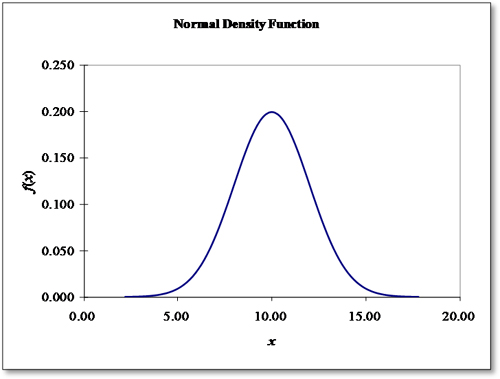
Parameter estimation: The sample mean and standard deviation are unbiased estimators of μ and σ.

Excel: In Excel, the standard normal distribution function evaluated at z is NORMSDIST(z). This is the probability that a standard normal random variable will be less than or equal to z. Excel normal density and distribution functions are NORMDIST(x, μ, σ, FALSE) and NORMDIST(x, μ, σ, TRUE). NORMINV(p, μ, σ) is the inverse distribution function, which returns the value of x that has cumulative probability p. Excel 2010 renames the functions as NORM.DIST, NORM.S.DIST, NORM.INV, and NORM.S.INV, but continue to use the same parameters.

Excel simulation: In an Excel simulation, normally distributed random variates can be generated by the inverse transform method with x = NORMINV(1-RAND(), μ, σ). Another approach, based on the central limit theorem, is to sum 12 random numbers. The sum minus 12 is approximately standard normal. The Box-Muller method is a special-purpose approach for generating independent normal random deviates from a stream of random numbers and is more efficient and precise than other methods. The Box-Muller VBA code follows:

---

---

Approximation for F(z): The following VBA code is an accurate approximation for the standard normal distribution function based on the algorithm in Press et al. (2002)³⁴. The author compared this approximation to NORMSDIST(z) for z in the range [−6, 6] and found a maximum absolute deviation of 7.45061×10^-8 at z = 0.72.

---

---

Approximation for the inverse distribution function F^-1(p): The following is an approximation for the inverse of the standard normal distribution function: x = F⁻¹(p) ≈ 5.06329114(p^0.135 − (1 − p)^0.135) or in Excel =5.06329114*(p ^0.135-(1-p)^0.135). This approximation was tested in Excel in the range p = (0.50400, 0.99997) and was found to have a maximum absolute percent error of 4.68% at p = 0.99997. For p in the range (0.504, 0.9987), the maximum absolute percent error was 0.67% at p = 0.10. Computer code for the inverse normal with a relative absolute error less than 1.15 × 10⁻⁹ for x = F⁻¹(p) −38 can be found at http://home.online.no/~pjacklam/notes/invnorm (April 7, 2011).

See binomial distribution, central limit theorem, confidence interval, error function, inverse transform method, lognormal distribution, probability density function, probability distribution, random number, sampling, Student’s t distribution.

normal time – A work measurement term from the field of industrial engineering used for the time to complete a task as observed from a time study, adjusted for the performance rating.

The steps in estimating a normal time are as follows:

1. Compute the average task time for each operator – Collect several random observations on task times, and compute the average observed task time for each operator i.

2. Estimate the performance rating for each operator – Make subjective estimates of the performance rating (r_i) for each operator i, where r_i = 1.10 for someone working 10% faster than normal.

3. Calculate the standard time – Calculate the standard time as the product of the allowance (A) and the average observed times adjusted by the performance ratings (r_i), i.e., . The allowance (A) is for personal needs, fatigue, and unavoidable delays. The allowance should depend on work environment issues, such as temperature, dust, dirt, fumes, noise, and vibration and is usually about 15%.

See performance rating, standard time, time study, work measurement, work sampling.

normalization – An information systems term for the process of reducing redundancies and anomalies in a database; once normalization is done, the database is said to be normalized.

See data warehouse.

North American Free Trade Agreement (NAFTA) – An agreement that formed a free trade area between the U.S., Canada, and Mexico. It went into effect on January 1, 1994.

np-chart – A statistical process control chart used to monitor the number of non-conforming units in a sample.

The np-chart is similar to a p-chart. The only major difference is that the np-chart uses count data rather than proportions. The control limits are typically set at , where p is the estimate of the long-term process mean. The np-chart plots the number of non-conforming units.

See control chart, p-chart, Poisson distribution, Statistical Process Control (SPC).

NPD – See New Product Development (NPD).

numerically controlled (NC) machine – See Computer Numerically Controlled (CNC) machine.

numeric-analytic location model – An iterative method that guarantees the optimal solution to the single facility infinite set location problem.

A firm needs to locate a single warehouse to serve n customers. Each customer (j) has coordinates (x_j, y_j), demand or weight (w_j), and a transportation cost of c_j per unit per mile. The single warehouse facility is to be located at the coordinates (x₀, y₀). The travel distance from the warehouse to customer j is assumed to be Pythagorean (straight-line) distance defined by . The goal is to find the (x₀, y₀) coordinates for the warehouse that minimize the total incremental cost (TIC) defined as . The center-of-gravity solution for this problem is and . This solution is sometimes called the “center of mass” or “centroid.” Although the center-of-gravity method is quite simple, it is not necessarily optimal and can be far from optimal.

See center-of-gravity model for facility location, facility location, gravity model for competitive retail store location, great circle distance, logistics, marginal cost, Pythagorean Theorem, warehouse.

O

objective function – See linear programming.

obsolescence – See obsolete inventory.

obsolete inventory – Inventory that can no longer be sold because of lack of market demand, outdated technology, degradation of quality, or spoilage; also called “dead and excess” inventory and “dead stock.”

Most firms try to remove obsolete inventory to free up space and take a tax write-off earlier rather than later. Firms often use simple rules to determine if inventory is dead. These rules are usually based on how much time has passed with no sales. Some firms, particularly retailers, can “clear” nearly obsolete inventory by selling it at a discounted price. Gupta, Hill, and Bouzdine-Chameeva (2006) presented a pricing model for clearing end-of-season retail inventory. Most firms have a financial reserve for obsolete inventory based on sales, current inventory investment, age, historical trends, and anticipated events.

See ABC classification, all-time demand, carrying charge, red tag, shrinkage, slow moving inventory, termination date.

OC curve – See operating characteristic curve.

Occam’s Razor – A principle in science and philosophy that recommends selecting the competing hypothesis that makes the fewest assumptions; also called the law of parsimony; also spelled Ockham’s Razor.

This principle is interpreted to mean that the simplest of two or more competing theories is preferable and that an explanation for unknown phenomena should first be attempted in terms of what is already known.

See KISS principle, parsimony.

Occupational Safety and Health Administration (OSHA) – A U.S. government agency created by the Occupational Safety and Health Act of 1970 to ensure safe and healthful working conditions for working men and women by setting and enforcing standards and by providing training, outreach, education and assistance.

OSHA is part of the U.S.Department of Labor. The administrator for OSHA is the assistant secretary of labor for occupational safety and health. OSHA’s administrator answers to the secretary of labor, who is a member of the cabinet of the president of the United States.

See DuPont STOP, error proofing, risk management, safety.

Ockham’s Razor – See Occam’s Razor.

OCR – See Optical Character Recognition (OCR).

ODM (Original Design Manufacturer) – See contract manufacturer.

OEE – See Overall Equipment Effectiveness.

OEM (Original Equipment Manufacturer) – See original equipment manufacturer.

off-line setup – See setup reduction.

offshoring – Developing a supplier in another country with either vertically integrated or external suppliers.

Whereas outsourcing refers to the use of another party regardless of that party’s location, offshoring refers to the location of the source of supply. A firm could offshore and own the offshore vertically integrated supplier.

The primary issues that should be considered in an offshore decision include (1) expertise in managing remote locations, (2) quality of the workforce, (3) cost of labor, (4) language skills, (5) telecom bandwidth, (6) cost and reliability, (7) infrastructure, (8) political stability, (9) enforceability of intellectual property rights and business contracts, (10) general maturity of the business environment, and (11) risk related to weather (earthquakes, hurricanes, tornadoes, typhoons, and volcanoes).

See expatriate, intellectual property (IP), landed cost, nearshoring, operations strategy, outsourcing, supply chain management.

one-minute manager – A simple managerial coaching concept that involves three one-minute interactions between a manager and an employee.

The One Minute Manager (Blanchard & Johnson 1982) presented three simple ways for managers to interact with their subordinates – goal setting, praise, and reprimand. All three of these interactions require about one minute, though the time may vary based on the situation. The main point is that these three interactions can and should be short, simple, and regular. These three interactions are briefly described below:

One-minute goal setting – One-minute managers regularly ask employees to review their goals with a script such as, “What are your goals for this month?” This process helps the manager and employees confirm that they are in complete agreement on goals and priorities.

One-minute praise – When one-minute managers catch their employees doing something right, they give their employees immediate praise and tell them specifically what they did right. Just saying “good job” is not specific. After giving a praise, the manager should pause for a moment to allow the employee to feel good and then remind the employee how his or her actions help the organization. The managers should finish by shaking hands and encouraging the employee to keep up the good work.

One-minute reprimand – One-minute managers provide immediate, specific, and clear feedback to employees. The goal of the reprimand is not to punish, but rather to help employees better achieve their goals. Following a reprimand, the manager should shake hands and remind the employee that he or she is important and that it was the employee’s behavior that did not meet the standard.

The three one-minute interactions are closely interrelated. One-minute goal setting clarifies goals, one-minute praise reinforces behavior consistent with the goals, and one-minute reprimand gives negative feedback for behavior inconsistent with the goals.

See management by walking around, SMART goals.

one-piece flow – A lean manufacturing practice of making only one part at a time (a batch size of one) before moving the part to the next step in the process; also called single-piece flow, make-one-move-one, and one-for-one replenishment.

This lean ideal is not always achievable. Single Minute Exchange of Dies and other setup time reduction methods are critical for helping organizations reduce setup cost (and ordering cost) and move toward this ideal.

See batch-and-queue, continuous flow, lean thinking, setup time reduction methods, Single Minute Exchange of Dies (SMED), zero inventory.

on-hand inventory – The quantity shown in the inventory records as being physically in the inventory.

Whereas on-hand inventory is the current physical quantity in stock, the inventory position is the quantity on-hand plus on-order, less allocated, less backordered.

See allocated inventory, backorder, cycle counting, inventory management, inventory position, Master Production Schedule (MPS), Materials Requirements Planning (MRP), on-order inventory, open order, perpetual inventory system.

on-order inventory – The amount of inventory that has been ordered from a supplier (internal or external) but not yet received.

The inventory position is the quantity on-hand, plus on-order, less allocated, less backordered.

See inventory management, inventory position, Master Production Schedule (MPS), Materials Requirements Planning (MRP), on-hand inventory, open order, perpetual inventory system.

on-the-job training (OJT) – A method for training employees by involving them in the work.

Workers develop skills simply by working, ideally under the watchful eye of a supervisor or mentor, and usually during the normal workday.

See cross-training, human resources, job design.

on-time and complete – See on-time delivery.

on-time delivery (OTD) – A customer delivery/service metric that is measured as the percentage of orders received by the promised date (within an allowable time window); also known as on-time and complete.

See blanket purchase order (PO), dispatching rules, operations performance metrics, service level, supplier scorecard, Transportation Management System (TMS).

open-book management – Sharing key financial information openly with employees and other stakeholders.

The phrase “open-book management” was coined by John Case of Inc. Magazine in 1993 (Aggarwal & Simkins 2001) to describe the practice of providing employees with all relevant information about their company’s financial performance. Some firms take it a step further and share financial information with customers and suppliers. In this author’s experience, this concept is rarely used in North America.

See stakeholder.

open order – An order sent to a supplier (either internal or external) but not yet received by the customer; also called a scheduled receipt.

When an order is sent to a supplier, it is said to be released. Open orders are included in the inventory position (but not the on-hand balance) and used with both internal and external suppliers. The on-order balance for an item is the sum of the order quantities for all open orders for that item.

See bullwhip effect, Business Requirements Planning (BRP), inventory position, net requirements, on-hand inventory, on-order inventory.

operating characteristic curve – A graphical approach for understanding the parameters of a lot acceptance sampling plan.

The operating characteristic curve (OC) plots the probability of accepting a lot on the y-axis and the lot fraction or percent defectives on the x-axis.

See acceptance sampling, consumer’s risk, producer’s risk, quality management, sampling, Statistical Process Control (SPC), Statistical Quality Control (SQC).

operation – (1) In a general context: Any manufacturing or service process, no matter how large or small. (2) In a Materials Requirements Planning (MRP) or shop floor control context: A specific step in the routing required to make an item.

In the MRP context, the routing specifies the sequence of operations required to make an item. Each operation is defined by the operation sequence number, the workcenter, required materials, standard setup time, and standard run time per part.

See dispatching rules, operations management (OM), routing, shop floor control.

operation overlapping – See transfer batch.

operations management (OM) – Management of the transformation process that converts labor, capital, materials, information, and other inputs into products and services for customers.

Operations management is a core subject taught in all business schools, along with accounting, finance, marketing, human resources, management information systems, and general management/strategy. The preface of this encyclopedia presents a framework for operations management. Many colleges and universities are now using the broader term “supply chain and operations management.”

The operations management framework below was developed through an extensive survey of operations management professors and practitioners (Hays, Bouzdine-Chameeva, Meyer Goldstein, Hill, & Scavarda 2007). (The figure below is an adaption of that framework.) An organization’s operations strategy is derived from its business strategy and should guide and inform decisions in the four “pillars” of operations management: product & process design, capacity & demand management, supply chain management, and process improvement. These four pillars are supported by quality and people management, systems management, analytical tools, and performance metrics. All terms in this framework are presented in detail elsewhere in this encyclopedia.

Operations management framework

Source: Professor Arthur V. Hill

The operations management profession is supported by many academic and professional societies, including:

• American Society for Quality (ASQ), www.asq.org

• APICS - The Association for Operations Management, www.apics.org

• Association for Manufacturing Excellence (AME), www.ame.org

• Council of Supply Chain Management Professionals (CSCMP), www.cscmp.org

• Decision Sciences Institute (DSI), www.decisionsciences.org

• European Operations Management Association (EurOMA), www.euroma-online.org

• Institute for Operations Research and the Management Sciences (INFORMS), www.informs.org

• Institute for Supply Management (ISM), www.ism.ws

• Institute of Industrial Engineers (IIE), www.iienet2.org

• International Federation of Operational Research Societies (IFORS), www.ifors.org

• Lean Enterprise Institute (LEI)³⁵, www.lean.org

• Manufacturing and Service Operations Management Society (MSOM), http://msom.society.informs.org

• Operational Research Society, www.orsoc.org.uk

• Production and Operations Management Society (POMS), www.poms.org

• Project Management Institute (PMI), www.pmi.org

• Society of Manufacturing Engineers (SME), www.sme.org

• Supply Chain Council (SCC)³⁶, www.supply-chain.org

A short description for each of these societies is presented in this encyclopedia. This list omits many other important professional societies in related disciplines inside and outside North America.

See American Society for Quality (ASQ), APICS (The Association for Operations Management), Association for Manufacturing Excellence (AME), Council of Supply Chain Management Professionals (CSCMP), Decision Sciences Institute (DSI), European Operations Management Association (EurOMA), human resources, Institute for Operations Research and the Management Sciences (INFORMS), Institute for Supply Management (ISM), Institute of Industrial Engineers (IIE), Manufacturing and Service Operations Management Society (MSOM), operation, operations research (OR), operations strategy, Production Operations Management Society (POMS), Project Management Institute (PMI), Society of Manufacturing Engineers (SME), Supply Chain Council.

operations performance metrics – Variables used to evaluate any process.

As noted in the balanced scorecard entry, it is important that the performance metrics be balanced. One way to balance metrics is to use both financial and operations performance metrics. Operations performance metrics are often the key means for achieving the financial performance metrics, because the operations performance metrics usually “drive” the financial metrics.

With respect to operations performance metrics, many firms have at least one metric in each of these three categories: better (quality related metrics), faster (time and flexibility related metrics), and cheaper (cost related metrics). Many operations experts argue that the cheaper metrics are improved by improving the better and faster metrics. This author has added stronger as a fourth category of metrics to include risk management and strategic alignment. Many operations performance metrics are used in practice. This encyclopedia provides clear definitions for nearly all of the following operations performance metrics:

Better metrics:

• Product performance metrics – These depend on the specific product (e.g., the specifications for an automobile will define how long it takes to accelerate from 0 to 60 miles per hour).

• Customer satisfaction and loyalty metrics – Customer satisfaction, intention to repurchase (willingness to return), willingness to recommend, Net Promoter Score (NPS), Customer Effort Score (CES), and actual customer loyalty.

• Process capability and performance metrics and quality metrics – Yield, defects, defects per million units, defects per million opportunities, parts per million, rolled throughput yield, sigma level metric, process capability (C_p), process capability index (C_pk), process performance (P_p), and the process performance index (P_pk).

• Service related metrics – Service level, cycle service level, unit fill rate, order fill rate, line fill rate, perfect order fill rate, on-time delivery (OTD), percent on-time and complete, average response time, premium freight, stockout cost, and shortage cost.

Faster metrics:

• Time metrics – Cycle time³⁷, order to cash cycle time, throughput time, customer leadtime, time to market, average wait time, average time in system, Mean Time to Repair (MTTR), Mean Time Between Failure (MTBF).

• Learning rate metrics – Learning rate (learning curve), half-life, and percent improvement.

• Theory of Constraints metrics – Inventory Dollar Days (IDD), Throughput Dollar Days (TDD), and Throughput dollars.

• Lean metrics – Value added ratio (also called manufacturing cycle effectiveness)³⁸.

Cheaper metrics:

• Inventory metrics – Inventory turnover, periods supply (days on-hand), inventory investment, and inventory carrying cost.

• Forecast error metrics – Mean Absolute Percent Error (MAPE), Mean Absolute Scaled Error (MASE), bias, and forecast attainment.

• Equipment metrics – Utilization, availability, downtime, first-pass yield, Mean Time Between Failure (MTBF), Mean Time to Repair (MTTR), and Overall Equipment Effectiveness (OEE).

• Traditional cost accounting metrics – Productivity (output/input), efficiency (standard time)/(actual time), utilization, sales, gross margin, overhead variance (fixed and variable), labor variance, labor efficiency variance, direct material variance, direct material price variance, and cost per part.

• Warehouse metrics – First pick ratio, inventory accuracy, capacity utilization, cube utilization, mispicks.

• Transportation metrics – Freight cost per unit shipped, outbound freight costs as percentage of net sales, inbound freight costs as percentage of purchases, average transit time, claims as percentage of freight costs, freight bill accuracy, percent of truckload capacity utilized, average truck turnaround time, on-time pickups.

Stronger metrics:

• Strategic alignment – Gap between goals and performance on highest level strategic performance metrics.

• Risk assessment metrics – Risk priority number (in the context of an FMEA), expected loss, probability of failure.

• Safety metrics – Number of days since last injury, number of serious accidents per time period, number of near misses, time to fix safety issues.

• Triple bottom line metrics – People (human capital) metrics, planet (natural capital) metrics, and profit (economic benefit for all stakeholders) metrics.

See balanced scorecard, benchmarking, Capability Maturity Model (CMM), cube utilization, Customer Effort Score (CES), cycle time, dashboard, Data Envelopment Analysis (DEA), downtime, efficiency, Failure Mode and Effects Analysis (FMEA), financial performance metrics, first pick ratio, forecast error metrics, half-life curve, Inventory Dollar Days (IDD), inventory turnover, Key Performance Indicator (KPI), learning curve, learning organization, Net Promoter Score (NPS), on-time delivery (OTD), Overall Equipment Effectiveness (OEE), performance management system, process capability and performance, productivity, queuing theory, robust, sand cone model, scales of measurement, service level, service management, sigma level, standard time, strategy map, supplier scorecard, Throughput Dollar Days (TDD), utilization, wait time, work measurement, yield, Y-tree.

operations research (OR) – The science that applies mathematical and computer science tools to support decision making.

Operations research (OR) draws on many mathematical disciplines, such as optimization, statistics, stochastic processes (queuing theory), decision theory, simulation, graph theory (network optimization), and game theory. Optimization can be further broken down into constrained and unconstrained optimization, each of which can be broken down further into linear, non-linear, and discrete optimization. Simulation appears to be a field of growing importance with a number of powerful software tools, such as Arena, that are available for creating complex stochastic models of real-world systems.

During its formative years shortly after World War II, OR professionals argued that OR projects should be multi-disciplinary. However, most OR people today are trained as mathematicians, computer scientists, or industrial engineers. OR is considered by most experts to be synonymous with management science. The largest professional organization for operations research is INFORMS (www.informs.org).

See algorithm, assignment problem, decision tree, genetic algorithm, heuristic, Institute for Operations Research and the Management Sciences (INFORMS), knapsack problem, linear programming (LP), Manufacturing and Service Operations Management Society (MSOM), mixed integer programming (MIP), network optimization, Newton’s method, operations management (OM), optimization, sensitivity analysis, simulated annealing, simulation, transportation problem, transshipment problem, Traveling Salesperson Problem (TSP).

operations strategy – A set of policies for using the firm’s resources to support the business unit’s strategy to gain competitive advantage; also called manufacturing strategy.

Operations objectives – Operations strategy is usually defined in terms of the operations objectives of cost, quality, flexibility, and service. Other variants of this list also include delivery (instead of service), time or speed (as a part of service or flexibility), and customization (as a type of flexibility). Some lists also include safety, sustainability, environmental issues, and development of human capital. The Andersen Corporation Menomonie plant uses safety, quality, delivery, cost, and morale. This encycleopedia uses better, faster, cheaper, and stronger, where stronger means more robust and better aligned with strategy.

Trade-offs – Firms can often gain competitive advantage by making the best tradeoffs and by avoiding trade-offs between operations objectives. For example, Dell Computer was able to “change the rules of the game” and gain competitive advantage by being the first to successfully offer low cost assemble-to-order customized computers through direct mail (providing customization and quality without cost). Similarly, FedEx was one of the first to offer reliable overnight package delivery at a reasonable price (providing reliable fast delivery at a reasonable price).

Explicit versus implicit – The operations strategy may be explicit or implicit. An implicit strategy is not written down, and senior executives may not be able to articulate it, but it becomes apparent with an objective evaluation of the management’s consistent approach to decision making and the firm’s position in the market.

Operations strategy process versus content – Researchers in the operations management field often make a distinction between the operations strategy process and content. The process is the methodology that the organization uses to create its operations strategy, whereas the content is the substance of the strategy.

Structure versus infrastructure decisions – The most effective operations organization is not necessarily the one that has the maximum efficiency, responsiveness, or flexibility, but rather the one that best fits the strategic requirements of the business. In other words, the operations organization should always strive to make decisions that are consistent with the competitive strategy being pursued by the strategic business unit. Hayes and Wheelwright (1984, p. 31) developed the following list of “manufacturing strategy decision categories” and divided the list into two sets – structure and infrastructure:

Whereas structural decisions are physical, longer term, and more difficult to change, infrastructural decisions are more tactical and require less visible capital investments (but can still be difficult to change). Hayes and Wheelwright argue that these eight decision areas are closely interrelated and that “it is this pattern of structural and infrastructural decisions that constitutes the manufacturing strategy of a business unit” (Hayes & Wheelwright 1984, p. 32). This framework is closely related to the McKinsey 7S Model.

Other entries in the EOM – The balanced scorecard, strategy map, and causal map entries discuss strategy process issues in more detail. The strategy map entry presents the time-based competition strategy. The mass customization entry presents customization as a potential component of an operations strategy. Outsourcing to achieve lower cost is also a component of an operations strategy. A focused factory is an important manufacturing strategy, and the Service Profit Chain is an important service operations strategy. The push-pull boundary and postponement entries deal with the customer interface, leadtime, and customization issues.

See 7S Model, agile manufacturing, balanced scorecard, blue ocean strategy, cash cow, catchball, competitive analysis, core competence, first mover advantage, five forces analysis, focused factory, industry analysis, mass customization, offshoring, operations management (OM), order qualifier, outsourcing, plant-within-a-plant, postponement, push-pull boundary, resource based view, respond to order (RTO), robust, sand cone model, Service Profit Chain, strategy map, supply chain management, sustainability, SWOT analysis, technology push, time-based competition, vertical integration, virtual organization.

opportunity cost – The value of an alternative (opportunity) that was not taken.

When people have a choice between two or more alternatives, they will generally choose the best one. However, choosing the best alternative means that they cannot choose the next best alternative. The opportunity cost is the value of the next best alternative that must be sacrificed, i.e., “the value of the road not taken.”

For example, a firm can only make one product in a factory and decides to build product A instead of B. Although it makes a profit on product A, it gave up the profit on product B. The forgone profit on product B is called the opportunity cost.

For a more specific example, consider a factory that has one large machine (the bottleneck) that constrains the plant’s production rate. The firm makes $1,000 per hour in gross revenue every hour the machine is running. The firm currently has a setup time on this machine of one hour per day, which means that the firm could make $1,000 more per day if the setup could be eliminated. The standard costing system assigns direct labor and overhead to this machine at a rate of $200 per machine hour. However, the true cost of the setup is much more than $200 per hour because of the opportunity cost (i.e., the lost gross margin).

See carrying cost, economics, overhead, setup cost, stockout, Theory of Constraints (TOC).

Optical Character Recognition (OCR) – A technology that enables a machine to translate images into text.

See Automated Data Collection (ADC), Electronic Product Code (EPC), lockbox.

optimization – An operations research term for mathematical techniques that find the best solution to a problem.

Optimization techniques can be classified as either unconstrained or constrained optimization. Unconstrained optimization methods include calculus and numerical methods (search methods). Constrained optimization methods include linear programming, integer programming, and many other mathematical programming methods. Optimization techniques can also be classified as deterministic (has no uncertainty) or stochastic (allows for uncertainty). For example, finding the optimal safety stock is usually modeled as an unconstrained stochastic optimization problem, and finding the minimum cost allocation of products to warehouses in a distribution network is usually modeled as a constrained deterministic optimization problem.

Although many students use the term “optimize” to describe any situation where they are attempting to find the best solution, most professors prefer to reserve the word to only describe situations where the mathematically best solution is guaranteed to be found by a mathematical optimization procedure.

Excel provides useful optimization tools with (1) Goal Seek (for unconstrained optimization) and (2) the Solver (for both unconstrained and constrained optimization). Excel can be used with the Solver (and VBA as needed) to develop practical decision support systems for many important supply chain and operations management optimization problems (Winston & Albright 2011).

See Advanced Planning and Scheduling (APS), algorithm, Decision Support System (DSS), genetic algorithm, heuristic, linear programming (LP), network optimization, operations research (OR), simulated annealing.

order backlog – See backlog.

order cost – The marginal cost of placing one more purchase or manufacturing order; synonymous with setup cost.

Order cost increases with the number of orders. It includes costs related to the work of preparing, shipping, releasing, monitoring, receiving inspection, and put away. The setup cost entry provides more details.

See inventory management, marginal cost, setup cost.

order cycle – The time between receipts for the orders of an item; also called the replenishment cycle.

The number of order cycles per year can be estimated as D/Q, where D is the forecasted annual demand and Q is the average order quantity. The reorder point entry presents a graph that shows several order cycles.

See reorder point, safety stock, service level, stockout.

order cycle service level – See safety stock.

order entry – The process (and the related organizational unit) of receiving customer sales order information and entering it into a fulfillment system.

Order entry systems communicate important information to customers, such as prices, terms, availability, promise dates, technical product information, and payment options (cash, credit, credit card, etc.). People taking orders (customer service representatives) may act as salespersons and pursue opportunities to cross-sell complimentary products and up-sell more expensive products. After the order has been entered into the system, the system will create information for picking, shipping, and invoicing.

See call center, configurator, cross-selling, customer service, fulfillment, functional silo.

order fill rate – See fill rate.

order fulfillment – See fulfillment.

order penetration point – See push-pull boundary.

order picking – See picking.

order point system – See reorder point.

order qualifier – An attribute of a product or service that is necessary for customers to consider buying; also called an order loser.

An order qualifier is a characteristic that customers use to screen products for further evaluation. In contrast, an order winner makes a critical difference in the buyer’s decision process. In other words, the order qualifier “gets the salesperson in the door” to be considered by the potential buyer and the order winner “gets the salesperson out the door with the order in hand” (i.e., seals the deal and beats out the competition).

For example, the order qualifier for some buyers looking for a watch might be a price under $100. However, the order winner might be other product characteristics, such as the warranty or the wristband.

See operations strategy.

order quantity modifier – See lotsizing methods.

order size – See lotsize.

order winner – See order qualifier.

order-to-cash – The time between the receipt of the order from the customer and the receipt of the payment from the customer.

See cycle time, respond to order (RTO).

order-up-to level – An inventory control term for a maximum inventory level; also called base stock, target inventory, max, maximum, model stock, and par level; in academic literature, often called an S system.

An inventory system using an order-up-to level policy calculates the order quantity as the order-up-to level minus the current inventory position. The optimal order-up-to level is the optimal safety stock plus the average demand per period times leadtime plus review period (i.e., T = SS + μ_d(L + P)). With a continuous review system, the review period is zero.

See inventory management, inventory position, joint replenishment, min-max inventory system, periodic review system, reorder point.

ordinal scale – See scales of measurement.

organizational design – (1) The structure that defines the duties, goals, decision rights, policies, and reporting relationships for individuals or groups of people in an organization. (2) The process of creating such a structure.

Organizational design structure – Although an organizational design is reflected in an organizational chart, it is much more than a chart. Some examples of organizational design structures include:

• Centralized structure – Decision rights are concentrated in the top management, and tight control is exercised over departments and divisions.

• Decentralized structure – Decision rights are distributed, and the departments and divisions have more autonomy.

• Hierarchical structure – A common centralized structure where clear reporting lines are drawn, with each manager typically having several direct reports.

• Functional structure – Organizations are divided along areas of expertise, such as engineering and marketing. This structure is usually efficient within functional areas.

• Divisional (product) structure – An example of a decentralized structure, where the organization is divided into geographical or product-based divisions.

• Matrix structure – A structure that uses cross-functional and cross-divisional teams to deliver products, where team members often report to both a functional boss and a project leader outside their function.

Organizational design process – Organizational design is the process of aligning the people in an organization to meet its strategic objectives. Organizational design activities start with the organization’s goals and take into account the current organizational structure, skills and abilities of its people, job functions, and uncertainty in the external environment. The process seeks to form the organization into a structure that best suits its value proposition.

See absorptive capacity, cross-functional team, High Performance Work Systems (HPWS), human resources, job design, job enlargement, RACI Matrix, self-directed work team, virtual organization, workforce agility.

organizational structure – See organizational design.

Original Design Manufacturer (ODM) – See contract manufacturer.

Original Equipment Manufacturer (OEM) – An organization that sells products made by other organizations under its own name and brand.

Contrary to what the name “original equipment manufacturer” suggests, the OEM is not the manufacturer, but rather the re-seller of the equipment to the end user. More fitting terms include “original equipment customizer,” “original equipment designer,” or “original equipment concept designer.” The OEM is usually the customizer or designer of the product and usually handles marketing, sales, and distribution. The OEM usually offers its own warranty, support, and licensing of the product.

In many cases, the OEM merely brands the equipment with its own logo. The OEM’s name is either placed on the devices by the manufacturer that makes the equipment or by the OEM itself. In some cases, the OEM does add value. For example, an OEM might purchase a computer from a company, combine it with its own hardware or software, and then sell it as a turnkey system (see Value Added Reseller).

Some firms specialize in OEM manufacturing but never sell anything under their own brands (see contract manufacturer). Many manufacturing companies have separate OEM divisions for goods that are private labeled.

The entry contract manufacturer discusses Electronics Manufacturing Services (EMS) and Contract Electronics Manufacturing Services (CEMS), which are special types of OEMs.

See contract manufacturer, private label, turnkey, Value Added Reseller (VAR).

OSHA – See Occupational Safety and Health Administration (OSHA).

outbound logistics – See logistics.

outlier – A statistical term used to describe an observed value that is out of the ordinary and therefore should not be included in the sample statistics.

Outliers can have a significant impact on the sample mean and variance. They can be attributed to either special causes (such as measurement error) or a heavy-tailed distribution. When outliers can be attributed to special causes, they should be removed from the sample. For example, this author set up a forecasting system for a firm that had a once-per-year shipment to Belgium. Removing this large planned shipment from the data made it easier to forecast the demand. A reasonable rule of thumb is to exclude observations that are above (below) the mean plus (minus) three standard deviations. However, it is foolish to exclude outliers from a sample unless the analyst has good theory behind doing so. In many cases, outliers provide important information about the distribution and the variable in question.

One approach for dealing with outliers is to use robust (error-resistant) statistics, such as the median. Unlike the mean, the median is not affected by a few outliers in the data. Other robust statistics include trimmed and Winsorized estimators and the interquartile range.

See control chart, interquartile range, linear regression, Mean Absolute Deviation (MAD), run chart, special cause variation, trim, trimmed mean, Winsorizing.

outsourcing – Buying products and services from an independent supplier.

Many popular articles imply that “outsourcing” is buying products or services from Asia or from some other part of the world. However, the correct definition of outsourcing is buying product or services from any outside firm. Sourcing products and services from a wholly owned subsidiary on another continent should be called “offshoring” rather than outsourcing; buying products or services from another firm on another continent should be called “offshore outsourcing.”

A good example of outsourcing is Boston Scientific’s clean room gowns. Boston Scientific’s core competence is designing, manufacturing, marketing, and selling implantable medical devices – not managing gowns. However, its gown supplier has a clear focus on clean room gowns and is “world class” at that business. Therefore, Boston Scientific outsources its gown management. An example of outsourcing services is Best Buy, which outsourced many of its IT and human resources functions to other firms.

Nearly all consultants and management professors argue that firms should not outsource their core competence. However, this statement is not always helpful, because many managers have trouble identifying their organization’s core competence and find that their core competence changes over time.

Some penetrating questions that managers should ask with respect to outsourcing include:

• If this process is a core competency, why are we making it only for ourselves? If a firm has a truly world-class process, then why not leverage that expertise (and overhead)? The answer to this question is often, “Well, the process is really not that good,” which suggests that the process is not a true core competence after all.

• If the process is not a core competency, why not buy it from someone who has this core competency? If a process is clearly not a core competence and never will be, then management should ask why not outsource it from another organization that has a core competency in this area?

• Are we ready to become dependent on others for this process? When outsourcing manufacturing, management is, in effect, deciding that the process is not a core competency and is creating dependency on other firms. When a firm outsources, it will no longer have those 20-year veterans who know everything there is to know about esoteric materials, equipment, and testing. The firm gives up the equipment, tools, and expertise. Over time, the firm may even erode its ability to talk intelligently to its suppliers and customers. This is not a significant problem as long as the process is clearly not a core competency and the firm has good suppliers who have this core competency.

• Do we understand the switching costs? Switching is often difficult and costly and involves many systems, such as machines, tooling, people, expertise, information systems, coordination, transportation, production planning, and costing. Moreover, switching back may be just as costly if management changes its mind.

Many firms find that they can improve both cost and quality if they can find an outside supplier that has a core competence in a particular area. For example, historically many firms have outsourced the manufacturing of components. More recently, we have seen firms outsourcing final assembly, new product development, and many services, such as IT and human resources.

Given that outsourcing often increases inventories, outsourcing can go against lean principles. For example, if a firm outsources a component to China and dramatically increases leadtimes, inventory and the associated carrying cost will also increase dramatically. Some experts consider Dell to be an example of successful lean outsourcing, because it outsources nearly all its component manufacturing and yet carries nearly zero component inventory³⁹. If managed properly, outsourcing, in combination with smart supplier agreements and Vendor Managed Inventories, can sometimes result in a significant decrease in inventories and provide excellent synergies with lean manufacturing.

Many firms fail to understand that many overhead costs do not go away (at least, not in the short term) with an outsourcing decision. Some of the “surprise” overhead costs that come with an outsourcing decision include:

• Overhead costs allocated to production in the high-wage location, which must be re-allocated to remaining products. In other words, some of the fixed costs do not go away in outsourcing, and the internal burden rates go up and the volume goes down. (See the make versus buy decision entry.)

• Carrying cost of the additional inventory of goods in transit (the square root law).

• Cost of additional safety stocks to ensure uninterrupted supply.

• Cost of expedited shipments.

• Cost of scrap-related quality issues.

• Cost of warranty claims if the new facility or supplier has a long learning curve.

• Cost of engineer visits to set up the operation or straighten out problems.

• Cost of stockouts and lost sales caused by long leadtimes.

• Cost of obsolete parts.

Outsourcing decisions sometimes also fail to properly account for currency risks, country risks, connectivity risks, and competitive risks when a supplier becomes a competitor.

Contracts are not always enforceable across international borders, particularly in countries that do not have well-developed legal systems. Therefore, the manufacturer will assume some risk with both the intellectual property (product designs and process designs) and during the order-to-cash cycle for any order. However, all business relationships involve risk, so it comes down to developing trust between the business partners. If the supplier wants to keep the manufacturer as a customer, it needs to prove itself trustworthy. Firms, on the other hand, need to weigh this risk against the risk of global competitors coming to the market with a significantly cheaper and better product.

The World Is Flat (Friedman 2005) identified ten forces that flattened the world and made offshore outsourcing much easier: (1) the fall of the Berlin Wall (11/9/89), (2) Netscape (8/9/95), (3) workflow software, (4) open-sourcing (blogs, wikis) allowing people to upload and collaborate, (5) outsourcing, (6) offshoring, (7) supply-chaining, (8) insourcing (B2B services)⁴⁰, (9) in-forming, and (10) wirelessness.

See absorptive capacity, Activity Based Costing (ABC), burden rate, business process outsourcing, carrying cost, contract manufacturer, co-packer, core competence, delegation, groupware, human resources, intellectual property (IP), labor intensive, landed cost, make versus buy decision, maquiladora, nearshoring, offshoring, operations strategy, overhead, purchasing, Service Level Agreement (SLA), sourcing, subcontracting, supply chain management, switching cost, vendor managed inventory (VMI), vertical integration.

Over/Short/Damaged Report – A transportation management report that highlights any items that were received but unexpected (i.e., more than what was ordered), expected but not received (i.e., short of what was ordered), or received in damaged condition; also called the OS&D report.

An Over/Short/Damaged report is commonly run for a single inbound trailer or for a day’s worth of inbound trailers to gauge the quality of the shipments. Ideally, an OS&D report should be completely empty with no unexpected, missing, or damaged items.

The OS&D report is typically created by the Transportation Management System or Warehouse Management System. The OS&D report is created by comparing the list of items the firm expected to receive (typically from the Advanced Shipping Notification) with the actual receipts as recorded by the warehouse personnel who handled the receiving. Often this OS&D report is created by comparing the barcode scans of the wireless devices used during receiving with the ASN file that defines what should have been in the trailer.

The OS&D report is important to managers for several reasons:

• Overage items will probably need manual intervention – Normally, in a cross-dock or warehousing scenario, each incoming item has an ultimate destination (typically another warehouse or some end shipping point). This destination is indicated in the ASN file. If an unexpected item is received in a high-volume cross-dock or warehousing environment, manual intervention will be required to determine the appropriate ultimate destination of the item.

• Missing items will need manual intervention – In normal circumstances, each item has an ultimate destination. If items are missing, warehouse managers may need to alert downstream warehouses or customers of missing goods.

• Proper recording of damages limits liability – In many logistics scenarios, the company takes ownership of the items only after they have been received in good condition. Any damage to items after receipt will be the responsibility of the recipient. Therefore, if damaged items are received, it is important that the damage be noted immediately. Good wireless Transportation Management Systems (TMS) and Warehouse Management Systems (WMS) make it easy for warehouse personnel to record damaged goods upon receipt.

From a high-level management perspective, the OS&D report can be used to evaluate the overall effectiveness of the relationship between the originator of the shipment and the recipient of the shipment.

See Advanced Shipping Notification (ASN), cross-docking, Electronic Data Interchange (EDI), logistics, receiving, shortage report, Transportation Management System (TMS), Warehouse Management System (WMS).

Overall Equipment Effectiveness (OEE) – A lean operations/TPM metric defined as the product of three variables – the availability rate, performance rate, and yield (or quality) rate.

Overall Equipment Effectiveness (OEE) is considered by many to be a key metric for lean operations management. OEE is used extensively in Total Productivity Management (TPM) applications, particularly in large firms, such as 3M, that have large capital intensive operations. OEE is the product of three variables: (Availability Rate) x (Performance Rate) x (Yield Rate). Each of these three variables is defined as follows:

• Availability rate = (Operating time less downtime)/(Total operating time). This measures downtime losses due to changeovers, equipment failures, and startup losses. Availability is not the same as utilization. Availability captures downtime losses from emergency maintenance, setups, and adjustments.

• Performance rate = (Total output)/(Potential output at rated speed). This measures speed losses due to idling and minor stoppages or reduced speed operation.

• Yield (or quality) rate = (Good output)/(Total output). This measures defects and rework. The yield rate for OEE is sometimes called the quality rate or first-pass yield rate.

If OEE is applied to a non-bottleneck machine, care must be taken to avoid maximizing utilization and building inventory long before it is needed. It does not make sense to maximize one asset (a machine) to create another asset (inventory) that sits idle for a long time. When properly implemented, OEE will maximize availability (which is not the same as utilization).

See capacity, downtime, effectiveness, efficiency, lean thinking, operations performance metrics, process capability and performance, productivity, rework, Total Productive Maintenance (TPM), utilization, value added ratio, yield.

overhead – Business costs that cannot be meaningfully and easily assigned to individual products or services; sometimes called indirect cost or burden.

Overhead costs include all costs to conduct business except for direct labor and direct materials. These costs include indirect labor, indirect materials, selling expenses, general and administrative expenses, depreciation, setup costs, quality costs, cleanup costs, fringe benefits, payrolls taxes, and insurance. Examples of overhead costs include the building and machine depreciation, building utilities (power, water, sewer), MRO supplies (e.g., sandpaper), office supplies (pens and paper), and supervisory labor. Manufacturing overhead is often allocated to products based on direct labor hours.

See absorption costing, Activity Based Costing (ABC), burden rate, carrying cost, commonality, cost of goods sold, direct cost, direct labor cost, job order costing, lean thinking, Maintenance-Repair-Operations (MRO), make versus buy decision, opportunity cost, outsourcing, period cost, setup cost, standard cost, Theory of Constraints (TOC), throughput accounting, variable costing, work measurement, Work-in-Process (WIP) inventory.

overhead rate – See burden rate.

overlapping – See transfer batch.

overproduction – Producing more than what is needed at the time.

See 8 wastes, batch-and-queue.