C

C&E diagram – A causal map using the Ishikawa (fishbone) diagram.

See C&E matrix, causal map, lean sigma, Root Cause Analysis (RCA), Root Cause Tree, seven tools of quality.

C&E Matrix – An analysis tool used to collect subjective data to make quantitative estimates of the impact of the Key Process Input Variables (KPIVs) on Key Process Output Variables (KPOVs) to identify the most important KPIVs for a process improvement program; also known as a cause and effect matrix.

In any process improvement program, it is important to determine which Key Process Input Variables (KPIVs) have the most impact on the Key Process Output Variables (KPOVs). The C&E Matrix is a practical way to collect subjective estimates of the importance of the KPIVs on the KPOVs.

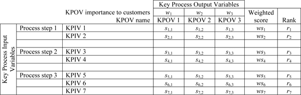
Building the C&E Matrix begins by defining the KPOVs along the columns on the top of the matrix (table) and the KPIVs along the rows on the left side. (See the example below.) Experts then estimate the importance of each KPOV to the customer. This is typically done on a 1-10 scale, where 1 is unimportant and 10 is critically important. Each pair of input and output variables is then scored on a 0-10 scale, where the score is the degree to which the input variable impacts (causes) the output variable. The sum of the weighted scores is then used to rank the input variables to determine which input variables deserve the most attention and analysis.

The example below illustrates the matrix for three KPOVs and seven KPIVs. KPOV 1 to KPOV 3 are the names of the output variables with customer importance weights (w₁, w₂, w₃). The s_i,j values are the impact scores for input (KPIV) variable i on output (KPOV) variable j. The weighted score for each KPIV is then calculated as the sum of the weights and the impact scores. Stated mathematically, the weighted score for the i-th KPIV is defined as , where J is the number of KPOVs. These scores are then ranked in the far right column.

C&E Matrix example

The C&E Matrix is closely related to the C&E Diagram and the causal map. The C&E Matrix is a special type of causal map represented in matrix form that has only one set of input variables (the KPIVs) and one set of output variables (the KPOVs). This can be generalized by including all variables on both rows and columns. This generalized matrix, called the adjacency matrix in the academic literature, allows for input variables to cause other input variables. This matrix can also be represented as a causal map. The “reachability” matrix is an extension of the adjacency matrix and represents how many steps it takes to get from one node to another in the network. Scavarda, Bouzdine-Chameeva, Goldstein, Hays, and Hill (2006) discussed many of these issues.

Some firms and consultants confuse a C&E Matrix with the Kepner-Tregoe Model (KT). KT is a simple scoring system for alternative courses of action, where each alternative is scored on a number of different dimensions, and each dimension has an assigned weight. The idea is that the alternative with the highest weighted sum is likely to be the best one. In contrast, the C&E Matrix scores input variables that cause output variables. In the KT Model, the dimensions do not cause the alternatives; they simply evaluate them.

See C&E Diagram, causal map, Kepner-Tregoe Model, Key Process Output Variable (KPOV), lean sigma.

CAD – See Computer Aided Design.

CAD/CAM – See Computer Aided Design/Computer Aided Manufacturing.

CAGR – See Compounded Annual Growth Rate (CAGR).

CAI – See Computer Aided Inspection.

call center – An organization that provides remote customer contact via telephone and may conduct outgoing marketing and telemarketing activities.

A call center can provide customer service such as (1) a help desk operation that provides technical support for software or hardware, (2) a reservations center for a hotel, airline, or other service, (3) a dispatch operation that sends technicians or other servers on service calls, (4) an order entry center that accepts orders for products from customers, and (5) a customer service center that provides other types of customer help.

A well-managed call center can have a major impact on customer relationships and on firm profitability. Call center management software monitors system status (number in queue, average talk time, etc.) and measures customer representative productivity. Advanced systems also provide forecasting and scheduling assistance. Well-managed call centers receive customer requests for help through phone calls, faxes, e-mails, regular mail, and information coming in through the Internet. Representatives respond via interpersonal conversations on the phone, phone messages sent automatically, fax-on-demand, interactive voice responses, and e-mails. Web-based information can provide help by dealing with a large percentage of common problems that customers might have and can provide downloadable files for customers. By taking advantage of integrated voice, video, and data, information can be delivered in a variety of compelling ways that enhance the user experience, encourage customer self-service, and dramatically reduce the cost of providing customer support.

The Erlang C formula is commonly used to determine staffing levels in any time period. (See the queuing theory entry for more information.)

See Automatic Call Distributor (ACD), cross-selling, customer service, help desk, knowledge management, order entry, pooling, queuing theory, service management, shrinkage.

CAM – See Computer Aided Manufacturing.

cannibalization – The sales of a new product that will be taken from the firm’s other products.

For example, a new computer model might take sales from an existing model and therefore add nothing to the firm’s overall market share or bottom line.

See market share.

cap and trade – A system of financial incentives put in place by the government to encourage corporations to reduce pollution.

The government issues emission permits that set limits (caps) for the pollution that can be emitted. Companies that produce fewer emissions can sell their excess pollution credits to those that produce more.

See carbon footprint, green manufacturing, sustainability.

capability – See Design for Six Sigma (DFSS), process capability and performance.

Capability Maturity Model (CMM) – A five-level methodology for measuring and improving processes.

CMM began as an approach for evaluating the “maturity” of software development organizations, but has since been extended to other organizations. Many capability maturity models have been developed for software acquisition, project management, new product development, and supply chain management. This discussion focuses on the Capability Maturity Model for Software (SW-CMM), which is one of the best-known products of the Carnegie Mellon University Software Engineering Institute (SEI). CMM is based heavily on the book Managing the Software Process (Humphries 1989). The actual development of the SW-CMM was done by the SEI at Carnegie Mellon University and the Mitre Corporation in response to a request to provide the federal government with a method for assessing the capability of its software contractors.

The SW-CMM model is used to score an organization on five maturity levels. Each maturity level includes a set of process goals. The five CMM levels follow:

Level 1: Initial – The software process is characterized as ad hoc and occasionally even chaotic. Few processes are defined and success depends on individual effort and heroics. Maturity level 1 success depends on having quality people. In spite of this ad hoc, chaotic environment, maturity level 1 organizations often produce products and services that work; however, they frequently exceed project budgets and schedules. Maturity level 1 organizations are characterized by a tendency to over-commit, abandon processes in the time of crisis, repeat past failures, and fail to repeat past successes.

Level 2: Repeatable – Basic project management processes are established to track cost and schedule activities. The minimum process discipline is in place to repeat earlier successes on projects with similar applications and scope. There is still a significant risk of exceeding cost and time estimates. Process discipline helps ensure that existing practices are retained during times of stress. When these practices are in place, projects are performed and managed according to their documented plans. Project status and the delivery of services are visible to management at defined points (for example, at major milestones and at the completion of major tasks).

Level 3: Defined – The software process for both management and engineering activities is documented, standardized, and integrated into a standard software process for the organization. All projects use an approved, tailored version of the organization’s standard software process for developing and maintaining software. A critical distinction between maturity levels 2 and 3 is the scope of standards, process descriptions, and procedures. At level 2, the standards, process descriptions, and procedures may be quite different in each specific instance of the process (for example, on a particular project). At maturity level 3, the standards, process descriptions, and procedures for a project are tailored from the organization’s set of standard processes to suit a particular project or organizational unit.

Level 4: Managed – Detailed measures of the software process and product quality are collected. Both the software process and products are quantitatively understood and controlled. Using precise measurements, management can effectively control the software development effort. In particular, management can identify ways to adjust and adapt the process to particular projects without measurable losses of quality or deviations from specifications. At this level, the organization sets a quantitative quality goal for both the software process and software maintenance. A critical distinction between maturity level 3 and maturity level 4 is the predictability of process performance. At maturity level 4, the process performance is controlled using statistical and other quantitative techniques and is quantitatively predictable.

Level 5: Optimizing – Maturity level 5 focuses on continually improving process performance through both incremental and innovative technological improvements. Quantitative process-improvement objectives for the organization are established, continually revised to reflect changing business objectives, and used as criteria in managing process improvement. The effects of deployed process improvements are measured and evaluated against the quantitative process-improvement objectives. Both the defined processes and the organization’s set of standard processes are targets of measurable improvement activities. Process improvements to address common causes of process variation and measurably improve the organization’s processes are identified, evaluated, and deployed. The organization’s ability to rapidly respond to changes and opportunities is enhanced by finding ways to accelerate and share learning. A critical distinction between maturity level 4 and maturity level 5 is the type of process variation addressed. At level 4, processes are concerned with addressing special causes of process variation and providing statistical predictability of the results. At level 5, processes are concerned with addressing common causes of process variation and changing the process to improve process performance (while maintaining statistical probability) and achieve the established quantitative process-improvement objectives.

Although these models have proven useful to many organizations, the use of multiple models has been problematic. Further, applying multiple models that are not integrated within and across an organization is costly in terms of training, appraisals, and improvement activities. The CMM Integration project (CMMI) was formed to sort out the problem of using multiple CMMs. The CMMI Product Team’s mission was to combine the following:

• The Capability Maturity Model for Software (SW-CMM) v2.0 draft C

• The Systems Engineering Capability Model (SECM)

• The Integrated Product Development Capability Maturity Model (IPD-CMM) v0.98

• Supplier sourcing

CMMI is the designated successor of the three source models. The SEI has released a policy to sunset the Software CMM and previous versions of the CMMI.

Many of the above concepts are from http://en.wikipedia.org/wiki/Capability_Maturity_Model #Level_1_-_Initial (November 4, 2006).

Interestingly, maturity level 5 is similar to the ideals defined in the lean sigma and lean philosophies.

See common cause variation, lean sigma, lean thinking, operations performance metrics.

capacity – (a) Process context: The maximum rate of output for a process, measured in units of output per unit of time; (b) Space/time/weight context: The maximum space or time available or the maximum weight that can be tolerated.

This entry focuses on definition (a). The unit of time may be of any length (a day, a shift, a minute, etc.). Note that it is redundant (and ignorant) to use the phrase “maximum capacity” because a capacity is a maximum.

Some sources make a distinction between several types of capacities:

Rated capacity, also known as effective capacity, nominal capacity, or calculated capacity, is the expected output rate for a process based on planned hours of operation, efficiency, and utilization. Rated capacity is the product of three variables, hours available, efficiency, and utilization.

Demonstrated capacity, also known as proven capacity, is the output rate that the process has actually been able to sustain over a period of time. However, demonstrated capacity is affected by starving (the process is stopped due to no input), blocking (the process is stopped because it has no room for output), and lack of market demand (we do not use capacity without demand).

Theoretical capacity is the maximum production rate based on mathematical or engineering calculations, which sometimes do not consider all relevant variables; therefore, it is quite possible that the capacity can be greater than or less than the theoretical value. It is fairly common for factories to work at 110% of their theoretical capacity.

Capacity should not be confused with load. If an elevator has three people on it, what is its capacity? This is a trick question. The capacity might be 2, 3, 20, or 99. If it has three people on it, the elevator has a current load of three and probably has a capacity of at least three. For many years, this author wrote APICS certification exam questions related to this concept. It was amazing how many people answered this question incorrectly.

The best capacity will minimize the total relevant cost, which is the sum of the capacity and waiting costs. All systems have a trade-off between capacity utilization and waiting time. These two variables have a nonlinear relationship. As utilization goes to 100%, the waiting time tends to go to infinity. Maximizing utilization is not the goal of the organization. The goal of capacity management is to minimize the sum of two relevant costs: the cost of the capacity and the cost of waiting.

For example, the optimal utilization for a fire engine is not 100%, but much closer to 1%. Utilization for an office copy machine should be relatively low because the cost of people waiting is usually higher than the cost of the machine waiting. One humorous question to ask students is: “Should you go make copies to keep the machine utilized?” The answer, of course, is “no” because utilization is not the goal. The goal, therefore, is to find the optimal balance between the cost of the machine and the cost of people waiting.

In contrast, some expensive machines, such as a bottling system, will run three shifts per day 365 days per year. The cost of downtime is the lost profit from the system and can be quite expensive.

In a manufacturing context, capacity management is executed at four levels: Resource Requirements Planning (RRP), Rough Cut Capacity Planning (RCCP), Capacity Requirements Planning (CRP), and input/output control. See those entries in this encyclopedia to learn more.

The newsvendor model can be used to find the optimal capacity. The model requires that the analyst define a time horizon, estimate the distribution of demand, and estimate the cost of having one unit of capacity too much and the cost of having one unit of capacity too little.

In some markets, customers can buy capacity rather than products. For example, a customer might buy the capacity of a supplier’s factory for one day per week. This can often help the customer reduce the procurement leadtime. Of course, if the customer does not use the capacity, the supplier will still be paid.

See absorptive capacity, bill of resources, bottleneck, capacity management, Capacity Requirements Planning (CRP), closed-loop MRP, downtime, input/output control, Little’s Law, load, newsvendor model, Overall Equipment Effectiveness (OEE), process design, queuing theory, Resource Requirements Planning (RRP), Rough Cut Capacity Planning (RCCP), safety capacity, utilization, yield management.

capacity cushion – See safety capacity.

capacity management – Planning, building, measuring, and controlling the output rate for a process.

See capacity.

Capacity Requirements Planning (CRP) – The planning process used in conjunction with Materials Requirements Planning (MRP) to convert open and planned shop orders into a load report in planned shop hours for each workcenter.

The CRP process is executed after the MRP planning process has produced the materials plan, which includes the set of all planned and open orders. CRP uses the order start date, order quantity, routing, standard setup times, and standard run times to estimate the number of shop hours required for each workcenter. It is possible for CRP to indicate that a capacity problem exists during specific time periods even when Resource Requirements Planning (RRP) and Rough Cut Capacity Planning (RCCP) have indicated that sufficient capacity is available. This is because RRP and RCCP are not as detailed as CRP with respect to timing the load. The output of the CRP process is the capacity plan, which is a schedule showing the planned load (capacity required) and planned capacity (capacity available) for each workcenter over several days or weeks. This is also called a load profile.

See Business Requirements Planning (BRP), capacity, closed-loop MRP, input/output control, Master Production Schedule (MPS), Materials Requirements Planning (MRP), planned order, Resource Requirements Planning (RRP), Rough Cut Capacity Planning (RCCP), routing, Sales & Operations Planning (S&OP).

capacity utilization – See utilization.

CAPEX – An abbreviation for the CAPital EXpenditure used as the initial investment in new machines, equipment, and facilities.

See capital.

capital – Money available for investing in assets that produce output.

See CAPEX, capital intensive.

capital intensive – Requiring a large expenditure of capital in comparison to labor.

A capital intensive industry requires large investments to produce a particular good. Good examples include power generation and oil refining.

See capital, labor intensive.

carbon footprint – A measure of the carbon dioxide (CO₂) and other greenhouse gas emissions released into the environment by a person, plant, organization, or state; often expressed as tons of carbon dioxide per year.

The carbon footprint takes into account energy use (heat, cooling, light, power, and refrigeration), transportation, and other means of emitting carbon.

See cap and trade, energy audit, green manufacturing, triple bottom line.

cargo – Goods transported by a vehicle; also called freight.

See logistics, shipping container.

carousel – A rotating materials handling device used to store and retrieve smaller parts for use in a factory or warehouse.

Carousels are often automated and used for picking small parts in a high-volume business. The carousel brings the part location to the picker so the picker does not have to travel to the bin location to store or retrieve a part. Both horizontal and vertical carousels are used in practice. The photo on the right is a vertical carousel.

See Automated Storage & Retrieval System (AS/RS), batch picking, picking, warehouse.

carrier – (1) In a logistics context: An organization that transports goods or people in its own vehicles. (2) In a telecommunications context: An organization that offers communication services. (3) In an insurance context: An organization that provides risk management services.

Carriers may specialize in small packages, less than truck load (LTL), full truck loads (TL), air, rail, or sea. In the U.S., a carrier involved in interstate moves must be licensed by the U.S. Department of Transportation. The shipper is the party that initiates the shipment.

See common carrier, for-hire carrier, less than truck load (LTL), logistics.

carrying charge – The cost of holding inventory per time period, expressed as a percentage of the unit cost.

This parameter is used to help inventory managers make economic trade-offs between inventory levels, order sizes, and other inventory control variables. The carrying charge is usually expressed as the cost of carrying one monetary unit (e.g., dollar) of inventory for one year and therefore has a unit of measure of $/$/year. Reasonable values are in the range of 15-40%.

The carrying charge is the sum of four factors: (1) the marginal cost of capital or the weighted average cost of capital (WACC), (2) a risk premium for obsolete inventory, (3) the storage and administration cost, and (4) a policy adjustment factor. This rate should only reflect costs that vary with the size of the inventory and should not include costs that vary with the number of inventory transactions (orders, receipts, etc.). A good approach for determining if a particular cost driver should be included in the carrying charge is to ask the question, “How will this cost be affected if the inventory is doubled (or halved)?” If the answer is “not at all,” that cost driver is probably not relevant (at least not in the short-term). It is difficult to make a precise estimate for the carrying charge. Many firms erroneously set it to the WACC and therefore underestimate the cost of carrying inventory.

See carrying cost, Economic Order Quantity (EOQ), hockey stick effect, inventory turnover, marginal cost, obsolete inventory, production planning, setup cost, shrinkage, weighted average.

carrying cost – The marginal cost per period for holding one unit of inventory (typically a year).

The carrying cost is usually calculated as the average inventory investment times the carrying charge. For example, if the annual carrying charge is 25% and the average inventory is $100,000, the carrying cost is $25,000 per year. Many firms incorrectly use the end-of-year inventory in this calculation, which is fine if the end-of-year inventory is close to the average inventory during the year. However, it is quite common for firms to have a “hockey stick” sales and shipment pattern where the end-of-year inventory is significantly less than the average inventory during the year. Technically, this type of average is called a “time-integrated average” and can be estimated fairly accurately by averaging the inventory at a number of points during the year.

Manufacturing and inventory managers must carefully apply managerial accounting principles in decision making. A critical element in many decisions is the estimation of the inventory carrying cost, sometimes called the “holding cost.” Typical decisions include the following:

• Service level trade-off decisions – Many make to stock manufacturers, distributors, and retailers sell standard products from inventory to customers who arrive randomly. In these situations, the firm’s service level improves with a larger finished goods inventory. Therefore, trade-offs have to be made between inventory carrying cost and service.

• Lot size decisions – A small order size requires a firm to place many orders, which results in a small “cycle” inventory. Assuming instantaneous delivery with order quantity Q, the average cycle inventory is approximately Q/2. Even though small manufacturing order sizes provide low average cycle inventory, they require more setups, which, in turn, may require significant capacity leading to a large queue inventory and a large overall carrying cost.

• Hedging and quantity discount decisions – Inventory carrying cost is also an important issue when evaluating opportunities to buy in large quantities or buy early to get a lower price. These decisions a total cost model to make evaluate the economic trade-offs between the carrying cost and the purchase price.

• In-sourcing versus outsourcing decisions – When trying to decide if a component or a product should be manufactured in-house or purchased from a supplier, the inventory carrying cost is often a significant factor. Due to longer leadtimes, firms generally increase inventory levels to support an outsourcing decision. It is important that the proper carrying cost be used to support this analysis.

The above decisions require a “managerial economics” approach to decision making, which means that the only costs that should be considered are those costs that vary directly with the amount of inventory. All other costs are irrelevant to the decision.

The carrying charge is a function of the following four variables:

• Cost of capital – Firms have alternative uses for money. The cost of capital reflects the opportunity cost of the money tied up in the inventory.

• Storage cost – The firm should consider only those storage costs that vary with the inventory level. These costs include warehousing, handling, insurance and taxes, depreciation, and shrinkage.

• Obsolescence risk – The risk of obsolescence tends to increase with inventory, particularly for firms that deal with high technology products, such as computers, or perishable products, such as food.

• Policy adjustment – This component of the carrying cost reflects management’s desire to pursue this policy and is based on management intuition rather than hard data.

When estimating the unit cost for the carrying cost calculation, most authors argue for ignoring allocated overhead. However, given that it is difficult for most organizations to know their unit cost without overhead, it is reasonable for them to use the fully burdened cost and use the appropriate carrying charge that does not double count handling, storage, or other overhead costs.

See carrying charge, Economic Order Quantity (EOQ), hockey stick effect, Inventory Dollar Days (IDD), inventory management, inventory turnover, marginal cost, materials management, opportunity cost, outsourcing, overhead, production planning, quantity discount, service level, setup cost, shrinkage, weighted average.

cash cow – The firm or business unit that holds a strong position in a mature industry and is being “milked” to provide cash for other business units; the cash cow is often in a mature industry and therefore not a good place for significant new investment.

The BCG Growth-Share Matrix⁶

Adapted by Professor Arthur V. Hill

The Boston Consulting Group (BCG) Growth-Share Matrix can help managers set investment priorities for the product portfolio in a business unit or for business units in a multidivisional firm. Stars are high growth/high market share products or business units. Cash cows have low growth but high market share and can be used to supply cash to the firm. Dogs have low growth and low market share and should be either fixed or liquidated. Question marks have high growth, but low market share; a few of these should be targeted for investment while the others should be divested. Stern and Deimler (2006) and Porter (1985) provide more detail.

See operations strategy.

Cash on Delivery (COD) – Contract terms that require payment for goods and transportation at time of delivery.

See FOB, terms, waybill.

casting – See foundry.

catchball – A lean term used to describe an iterative top-down/bottom-up process in which plans are “thrown” back and forth between two levels in an organization until the participants at the different levels come to a shared understanding.

The term “catchball” is a metaphor used in the hoshin planning process for participative give-and-take discussions between two levels of an organization when creating a strategic plan. Catchball can help an organization achieve buy-in, find agreement, build a shared understanding, and create detailed execution plans for both the development and execution of a strategy. Catchball is “played” between multiple levels of the organization to ensure that the strategic plan is embraced and executable at every level.

The strategic planning process in many organizations has two common issues: (1) the plan is difficult to implement because the higher-level management is out of touch with the details, and (2) the lower-level managers do not understand the rationale behind the plan and therefore either passively resist or actively oppose the new strategy. With catchball, higher-level management develops a high-level plan and then communicates with the next layer of management to gain understanding and buy-in. Compared to other types of strategic planning, catchball usually results in strategic plans that are embraced by a wider group of managers and are more realistic (e.g., easier to implement).

Catchball essentially has two steps: (1) conduct an interactive session early in the planning process to give the next level of management the opportunity to ask questions, provide feedback, and challenge specific items, and (2) have the next level managers develop an execution plan for the higher-level initiatives and toss it back to the higher-level managers for feedback and challenges.

Catchball is comparable to agile software development where software ideas are tested early and often, which leads to better software. The same is true for strategy development with catchball where strategic plans are tested early and often. Both concepts are similar to the idea of small lotsizes and early detection of defects.

See agile software development, early detection, hoshin planning, lean thinking, operations strategy, prototype.

category captain – A role given by a retailer to a representative from a supplier to help the retailer manage a category of products.

It is a common practice for retailers in North America to select one supplier in a category as the category captain. A retailer usually (but not always) selects the category captain as the supplier with the highest sales in the category. The supplier then selects an individual among its employees to serve in the category captain’s role. Traditionally, the category captain is a branded supplier; however, the role is sometimes also given to private label suppliers. Category captains often have their offices at the customer’s sites.

The category captain is expected to work closely with the retailer to provide three types of services:

Analyze data:

• Analyze category and channel data to develop consumer and business insights across the entire category.

• Perform competitive analyses by category, brand, and package to identify trends.

• Analyze consumer purchasing behavior by demographic profile to understand consumer trends by channel.

• Audit stores.

Develop and present plans:

• Develop business plans and strategies for achieving category volume, margin, share, space, and profit targets.

• Help the retailer build the planogram for the category.

• Prepare and present category performance reviews for the retailer.

• Participate in presentations as a credible expert in the category.

Support the retailer:

• Respond quickly to the retailer’s requests for information.

• Provide the retailer with information on shelf allocation in a rapidly changing environment.

• Educate the retailer’s sales teams.

• Advise the retailer on shelving standards and associated software tools.

Craig Johnson, a Kimberly-Clark category captain at Target, adds, “Most category captains also have responsibilities within their own company as well and have to balance the needs of their retailer with internal company needs. It can get hairy sometimes.”⁷

The category captain must focus on growing the category, even if requires promoting competing products and brands. This practice will lead to the growth of the entire category and therefore be in the best interests of the supplier. In return for this special relationship, the supplier will have an influential voice with the retailer. However, the supplier must be careful never to abuse this relationship or violate any antitrust laws.

The category captain is usually given access to the retailer’s proprietary information, such as point-of-sale (POS) data. This information includes sales data for all suppliers that compete in the category. The retailer and category captain will usually have an explicit agreement that requires the captain to use this data only for category management and not share it with anyone in the supplier’s company.

Retailers will sometimes assign a second competing supplier as a category adviser called the “category validator.” In theory, the validator role was created as a way for the retailer to compare and evaluate the category captain’s recommendations. In practice, however, the adviser is usually used by the retailer as another category management resource. The adviser conducts ad hoc category analyses at the request of the retailer, but does not usually duplicate the services provided by the captain.

See antitrust laws, assortment, category killer, category management, consumable goods, consumer packaged goods, Fast Moving Consumer Goods (FMCG), planogram, Point-of-Sale (POS), private label.

category killer – A term used in marketing and strategic management to describe a dominant product or service that tends to have a natural monopoly in a market.

One example of a category killer is eBay, an on-line auction website that attracts large numbers of buyers and sellers simply because it is the largest on-line auction. Other examples include “big box” retailers, such as Home Depot, that tend to drive smaller “mom and pop” retailers out of business.

See big box store, category captain, category management.

category management – The retail practice of segmenting items (SKUs) into groups called categories to make it easier to manage assortments, inventories, shelf-space allocation, promotions, and purchases.

Benefits claimed for a good category management system include increased sales due to better space allocation and better stocking levels, lower cost due to lower inventories, and increased customer retention due to better matching of supply and demand. Category management in retailing is analogous to the commodity management function in purchasing.

See assortment, brand, category captain, category killer, commodity, consumable goods, consumer packaged goods, Fast Moving Consumer Goods (FMCG), private label.

category validator – See category captain.

causal forecasting – See econometric forecasting, forecasting.

causal map – A graphical tool often used for identifying the root causes of a problem; also known as a cause and effect diagram (C&E Diagram), Ishikawa Diagram, fishbone diagram, cause map, impact wheel, root cause tree, fault tree analysis, and current reality trees.

A causal map is a diagram that shows the cause and effect relationships in a system. Causal maps can add value to organizations in many ways:

• Process improvement and problem solving – Causal maps are a powerful tool for gaining a deep understanding of any problem. As the old adage goes, “A problem well-defined is a problem half-solved.” The causal map is a great way to help organizations understand the system of causes that result in blocked goals and then find solutions to the real problems rather than just the symptoms of the problems. People think in “visual” ways. A good causal map is worth 1000 words and can significantly reduce meeting time and the time to achieve the benefit from a process improvement project.

• Supporting risk mitigation efforts – Causal maps are a powerful tool for helping firms identify possible causes of problems and develop risk mitigation strategies for these possible causes.

• Gaining consensus – The brainstorming process of creating a causal map is also a powerful tool for “gaining a shared understanding” of how a system works. The discussion, debate, and deliberation process in building a causal map is often more important than the map itself.

• Training and teaching – A good causal map can dramatically reduce the time required to communicate complex relationships for training, teaching, and documentation purposes.

• Identifying the critical metrics – Many organizations have too many metrics, which causes managers to lose sight of the critical variables in the system. A good causal map can help managers identify the critical variables that drive performance and require high-level attention. Focusing on these few critical metrics leads to strategic alignment, which in turn leads to organizational success.

Many types of causal maps are used in practice, including Ishikawa Diagrams (also known as fishbone diagrams, cause and effect diagram, and C&E Diagrams), impact wheels (from one cause to many effects), root cause trees (from one effect to many causes), and strategy maps. The Ishikawa Diagram was developed by Dr. Kaoru Ishikawa (1943-1969) and is by far the most popular form of a causal map. The Ishikawa Diagram is a special type of a causal map that shows the relationships between the problem (at the “head” of the fishbone on the right) and the potential causes of a problem. The figure below is a simple example of an Ishikawa Diagram for analyzing long waiting lines for tellers in a bank.

The Ishikawa Diagram is usually developed in a brainstorming context. The process begins by placing the name of a basic problem of interest at the far right of the diagram at the “head” of the main “backbone” of the fish. The main causes of the problem are drawn as bones off the main backbone. Many firms prescribe six causes: machines (equipment), methods, measurement, materials, manpower (labor), and Mother Nature (environment). However, many argue that this list is overly confining and a bit sexist. Brainstorming is typically done to add possible causes to the main bones and more specific causes to the bones on the main bones. This subdivision into ever-increasing specificity continues as long as the problem areas can be further subdivided. The practical maximum depth of this tree is usually about four or five levels.

Ishikawa Diagram example

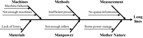
Source: Arthur V. Hill

The Ishikawa Diagram is limited in many ways:

• It can only analyze one output variable at a time.

• Some people have trouble working backward from the problem on the far right side of the page.

• It is hard to read and even harder to draw, especially when the problem requires many levels of causation.

• The diagram is also hard to create on a computer.

• The alliteration of Ms is sexist with the terms “manpower” and “Mother Nature.”

• The six Ms rarely include all possible causes of a problem.

Causal maps do not have any of these limitations.

The Ishikawa Diagram starts with the result on the right. With root cause trees, current reality trees (Goldratt 1994), and strategy maps (Kaplan & Norton 2004), the result is usually written at the top of the page. With an FMEA analysis and issues trees, the result is written on the left and then broken into its root causes on the right.

The causal map diagram below summarizes the 304-page book Competing Against Time (Stalk & Hout 2003) in less than a half-page. This is a strategy map using a causal map format rather than the Kaplan and Norton (1992) four-perspective strategy map format. This time-based competition strategy reduces cycle times, cost, and customer leadtimes. Reducing customer leadtimes segments the market, leaving the price-sensitive customers to the competition. This strategy map could be taken a step further to show how the firm could achieve lower cycle time through setup time reduction, vendor relationships, 5S, and plant re-layout.

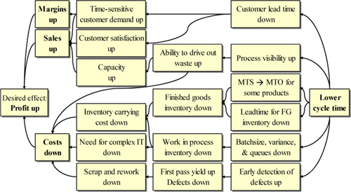
Source: Professor Arthur V. Hill

Regardless of the format used, these diagrams are usually created through a brainstorming process, often with the help of 3M Post-it Notes. The team brainstorms to identify the root causes of each node. The process continues until all causes (nodes) and relationships (arcs) have been identified. It is possible that “loops” will occur in the diagram. A loop can occur for a vicious cycle or virtuous cycle. For example, a vicious cycle occurs when an alcoholic person drinks and is criticized by family members, which may, in turn, cause him or her to drink even more, be criticized further, etc. A virtuous cycle is similar, except that the result is positive instead of negative.

Scavarda, Bouzdine-Chameeva, Goldstein, Hays, and Hill (2006) developed a method for building collective causal maps with a group of experts. This method assigns weights to each causal relationship and results in a meaningful graphical causal map, with the more important causal relationships shown with darker arrows.

Many software tools are available to help brainstorm and document the cause and effect diagrams. However, Galley (2008) insists that Excel is the best tool.

The C&E Matrix provides a means for experts to assign weights to certain causal input variables. The same can be done with a causal map. All that needs to be done is to score each input variable on several dimensions that are important to customers and then create a weighted score for each input variable. Priority is then given to those variables that are believed to have the most impact on customers. Alternatively, experts can “vote” (using multi-voting) for the causes that they believe should be the focus for further analysis.

Causal maps should not be confused with concept maps, knowledge maps, and mindmaps that nearly always show similarities (but not causality) between objects. For example, monkeys and apes are very similar, but monkeys do not cause apes. Therefore, a knowledge map would show a strong connection between monkeys and apes, but a causal map would not.

Hill (2011b, 2011c) provides more detail on this subject.

See 5 Whys, affinity diagram, Analytic Hierarchy Process (AHP), balanced scorecard, brainstorming, C&E Diagram, C&E Matrix, current reality tree, decision tree, Failure Mode and Effects Analysis (FMEA), fault tree analysis, future reality tree, hoshin planning, ideation, impact wheel, issue tree, lean sigma, MECE, mindmap, Nominal Group Technique (NGT), Pareto Chart, Pareto’s Law, parking lot, process map, quality management, Root Cause Analysis (RCA), root cause tree, sentinel event, seven tools of quality, strategy map, Total Quality Management (TQM), value stream map, Y-tree.

cause and effect diagram – See causal map.

cause map – A trademarked term for a causal map coined by Mark Galley of ThinkReliability.

Cause mapping is a registered trademark of Novem, Inc., doing business as ThinkReliability (www.thinkreliability.com).

See causal map.

caveat emptor – A Latin phrase that means “buyer beware” or “let the buyer beware.”

This phrase means that the buyer (not the seller) is at risk with a purchase decision. The phrase “caveat venditor” is Latin for “let the seller beware.”

See service guarantee, warranty.

CBT – See Computer Based Training (CBT).

c-chart – A quality control chart used to display and monitor the number of defects per sample (or per batch, per day, etc.) in a production process.

Whereas a p-chart controls the percentage of units that are defective, a c-chart controls the number of defects per unit. Note that one unit can have multiple defects. The Poisson distribution is typically used for c-charts, which suggests that defects are rare.

See attribute, control chart, Poisson distribution, Statistical Process Control (SPC), Statistical Quality Control (SQC), u-chart.

CDF – See probability density function.

cell – See cellular manufacturing.

cellular manufacturing – The use of a group of machines dedicated to processing parts, part families, or product families that require a similar sequence of operations.

Concept – In a traditional functional (process) layout, machines and workers are arranged in workcenters by function (e.g., drills or lathes), large batches of parts are moved between workcenters, and workers receive limited cross-training on the one type of machine in their workcenter. With cellular manufacturing, machines and workers are dedicated to making a particular type of product or part family. The machines in the cell, therefore, are laid out in the sequence required to make that product. With cells, materials are moved in small batches and workers are cross-trained on multiple machines and process steps. Cells are often organized in a Ushaped layout so workers inside the “U” can communicate and help each other as needed. The figure below contrasts functional and cellular layouts showing that cells can have a much higher value added ratio.

Functional (process) layout

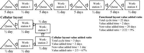
Source: Arthur V. Hill

Advantages of a cell over a product layout – The advantages of a cell over a product layout include reduced cycle time, travel time, setup time, queue time, work-in-process inventory, space, and materials handling cost. Reduced cycle time allows for quicker detection of defects and simpler scheduling. When firms create cells, they often cross-train workers in a cell, which leads to better engagement, morale, and labor productivity. Some firms also implement self-managed work teams to develop workers, reduce overhead, and accelerate process improvement.

Disadvantages of a cell over a product layout – The main disadvantage of a cell is that the machines dedicated to a cell may not have sufficient utilization to justify the capital expense. Consequently, cellular manufacturing is often difficult to implement in a facility that uses large expensive machines. When a firm has one very large expensive machine, it might still use cells for all other steps.

Professors Nancy Hyer and Urban Wemmerlov wrote a book and an article on on using cells for administrative work (Hyer & Wemmerlov 2002a, 2002b).

See automation, Chaku-Chaku, cross-training, facility layout, Flexible Manufacturing System (FMS), focused factory, group technology, handoff, job design, lean thinking, product family, utilization, value added ratio, workcenter, Work-in-Process (WIP) inventory.

CEMS (Contract Electronics Manufacturing Services) – See contract manufacturer.

censored data – Data that is incomplete because it does not include a subpopulation of the data.

A good example of censored data is demand data that does not include data for lost sales. A retailer reports that the sales were 100 for a particular date. However, the firm ran out of stock during the day and does not have information on how many units were demanded but not sold due to lack of inventory. The demand data for this firm is said to be “censored.”

See demand, forecasting.

centered moving average – See exponential smoothing, moving average.

center-of-gravity model for facility location – A method for locating a single facility on an x-y coordinate system to attempt to minimize the weighted travel distances; also called the center of mass or centroid model.

This is called the “infinite set” facility location problem because the “depot” can be located at any point on the x-y coordinate axis. The model treats the x and y dimensions independently and finds the first moment in each dimension. The one depot serves N markets with locations at coordinates (x_i, y_i) and demands D_i units.

The center-of-gravity location for the depot is then and .

This model does not guarantee optimality and can only locate a single depot. Center-of-gravity locations can be far from optimal. In contrast, the numeric-analytic location model guarantees optimality for a single depot location, can be extended (heuristically) to multiple depots, and can also be extended (heuristically) to multiple depots with latitude and longitude data.

See facility location, gravity model for competitive retail store location, numeric-analytic location model.

central limit theorem – An important probability theory concept that can be stated informally as “The sum or average of many independent random variables will be approximately normally distributed.”

For example, the first panel in the figure below shows a probability distribution (density function) that is clearly non-normal. (This is the triangular density function.) The second figure shows the distribution of a random variable that is the average of two independent random variates drawn from the first distribution.

The third and fourth figures show the probability distributions when the number of random variates in the average increases to four and eight. In each successive figure, the distribution for the average of the random variates is closer to normal. This example shows that as the number of random variates in the average increases, the distribution of the average (and the sum) converges to the normal distribution.

Central limit theorem example

Source: Professor Arthur V. Hill

See confidence interval, Law of Large Numbers, normal distribution, sample size calculation, sampling, sampling distribution.

certification – See supplier qualification and certification.

CGS (Cost of Goods Sold) – See cost of goods sold.

chain of custody – See traceability.

Chaku-Chaku – The Japanese phrase “Load, Load” used to describe the practice of facilitating one-piece flow in a manufacturing cell, where equipment automatically unloads parts so the operator can move parts between machines with minimal wasted motion.

With Chaku-Chaku, the operator is responsible for moving parts from machine to machine around an oval or circular-shaped cell and also for monitoring machine performance. When arriving at a machine in the cell, the operator will find a completed part already removed from the machine and the machine ready for a new part. The operator then starts a new part (from the previous machine), picks up the completed part from the machine, and then carries the part to the next machine in the cell to repeat the process.

See cellular manufacturing, multiple-machine handling.

champion – A senior manager who sponsors a program or project; also called an executive sponsor or sponsor.

The champion’s role is to define the strategic direction, ensure that resources are available, provide accountability, and deal with political resistance. This term is often used in the context of a process improvement program at both the program level (the program champion) and the project level (the project sponsor). Although the role can be either formal or informal, in many contexts, making it formal has significant benefits.

See deployment leader, lean sigma, lean thinking, program management office, project charter, sponsor.

change management – A structured approach for helping individuals, teams, and organizations transition from a current state to a desired future state.

Change management is an important discipline in a wide variety of project management contexts, including information systems, process improvement programs (e.g., lean sigma), new product development, quality management, and systems engineering. Organizational change requires (1) helping stakeholders overcome resistance to change, (2) developing new consensus, values, attitudes, norms, and behaviors to support the future state, and finally (3) reinforcing the new behaviors through new organizational structures, reward systems, performance management systems, and standard operating procedures. The benefits of good change management include better engagement of workers, reduced risk of project failure, reduced time and cost to affect the change, and longer lasting results.

The ADKAR Model for Change and the Lewin/Schein Theory of Change entries in this encyclopedia present specific change management methodologies.

See ADKAR Model for Change, co-opt, Lewin/Schein Theory of Change, project charter, project management, RACI Matrix, stakeholder analysis.

changeover – See setup.

changeover cost – See setup cost.

changeover time – See setup time.

channel – See distribution channel.

channel conflict – Competition between players trying to sell to the same customers.

For example, a personal computer company might try to compete with its own distributors (such as Sears) for customers by selling directly to customers. This is often an issue when a retail channel is in competition with a Web-based channel set up by the company. Channel conflict is not a new phenomenon with the Internet, but has become more obvious with the disruptions caused by the Internet.

See disintermediation, distribution channel, distributor, supply chain management.

channel integration – The practice of extending strategic alliances to the suppliers (and their suppliers) and to customers (and to their customers).

See distribution channel, supply chain management.

channel partner – A firm that works with another firm to provide products and services to customers.

Channel partners for a manufacturing firm generally include distributors, sales representatives, logistics firms, transportation firms, and retailers. Note that the term “partner” is imprecise because relationships with distributors and other “channel partners” are rarely legal partnerships.

See distribution channel, supply chain management.

chargeback – See incoming inspection.

chase strategy – A production planning approach that changes the workforce level to match seasonal demand to keep finished goods inventory relatively low.

With the chase strategy, the workforce level is changed to meet (or chase) demand. In contrast, the level strategy maintains a constant workforce level and meets demand with inventory (built in the off-season), overtime production, or both.

Many firms are able to economically implement a chase strategy for each product and a level employment overall strategy by offering counter-seasonal products. For example, a company that makes snow skis might also make water skis to maintain a constant workforce without building large inventories in the off-season. Other examples of counter-seasonal products include snow blowers and lawn mowers (Toro Company) and snowmobiles and all terrain vehicles (Polaris).

See heijunka, level strategy, Master Production Schedule (MPS), production planning, Sales & Operations Planning (S&OP), seasonality.

Chebyshev distance – See Minkowski distance.

Chebyshev’s inequality – A probability theory concept stating that no more than 1/k² of a distribution can be more than k standard deviations away from the mean.

This theorem is named for the Russian mathematician Pafnuty Lvovich Chebyshev (). The theorem can be stated mathematically as and can be applied to all probability distributions. The one-sided Chebyshev inequality is P(X − μ kσ) 1/(1 + k²).

See confidence interval.

check digit – A single number (a digit) between 0 and 9 that is usually placed at the end of an identifying number (such as a part number, bank account, credit card number, or employee ID) and is used to perform a quick test to see if the identifying number is clearly invalid.

The check digit is usually the last digit in the identifying number and is computed from the base number, which is the identifying number without the check digit. By comparing the check digit computed from the base number with the check digit that is part of the identifying number, it is possible to quickly check if an identifying number is clearly invalid without accessing a database of valid identifying numbers. This is particularly powerful for remote data entry of credit card numbers and part numbers. These applications typically have large databases that make number validation relatively expensive. However, it is important to understand that identifying numbers with valid check digits are not necessarily valid identifying numbers; the check digit only determines if the identifying number is clearly invalid.

A simple approach for checking the validity of a number is to use the following method: Multiply the last digit (the check digit) by one, the second-to-last digit by two, the third-to-last digit by one, the fourth-to-last digit by two, etc. Then sum all digits in these products (including the check digit), divide by ten, and find the remainder. The number is proven invalid if the remainder is not zero.

For example, the account number 5249 has the check digit 9. The products are 1 × 9 = 9, 2 × 4 = 8, 1 × 2 = 2, and 2 × 5 = 10. The sum of the digits is 9 + 8 + 2 + 1 + 0 = 20, which is divisible by 10 and therefore is a valid check digit. Note that the procedure adds the digits, which means that 10 is treated as 1 + 0 = 1 rather than a 10. The above procedure works with most credit card and bank account numbers.

The check digit for all books registered with an International Standard Book Number is the last digit of the ISBN. The ISBN method for the 10-digit ISBN weights the digits from 10 down to 1, sums the products, and then returns the check digit as modulus 11 of this sum. An upper case X is used in lieu of 10.

For example, Operations Management for Competitive Advantage, Eleventh Edition by Chase, Jacobs, and Aquilano (2006) has ISBN 0-07-312151-7, which is 0073121517 without the dashes. The ending “7” is the check digit so the base number is 007312151. Multiplying 10 × 0 = 0, 9 × 0 = 0, 8 × 7 = 56, 7 × 3 = 21, 6 × 1 = 6, 5 × 2 = 10, 4 × 1 = 4, 3 × 5 = 15, and 2 × 1 = 2 and adding the products 0 + 0 + 56 + 21 + 6 + 10 + 4 + 15 + 2 = 114. Dividing 114 by 11 has a remainder of 7, which is the correct check digit. The new 13-digit ISBN uses a slightly different algorithm.

See algorithm, part number.

checklist – A record of tasks that need to be done for error proofing a process.

A checklist is a tool that can be used to ensure that all important steps in a process are done. For example, pilots often use maintenance checklists for items that need to be done before takeoff. The 5S discipline for a crash cart in a hospital uses a checklist that needs to be checked each morning to ensure that the required items are on the cart. Checklists are often confused with checksheets, which are tally sheets for collecting data.

See checksheet, error proofing, multiplication principle.

checksheet – A simple approach for collecting defect data; also called a tally sheet.

A checksheet is a simple form that can be used to collect and count defects or other data for a Pareto analysis. It is considered one of the seven tools of quality. The user makes a check mark () every time a defect of a particular type occurs in that time period. The table below provides a simple example of a checksheet that records the causes for machine downtime.

Checksheet example

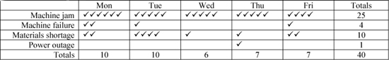
A different format for a checksheet shows a drawing (schematic) of a product (such as a shirt) and counts the problems with a checkmark on the drawing in the appropriate location. For example, if a defect is found on the collar, a checkmark is put on a drawing of a shirt by the shirt collar.

Checksheets should be used in the gemba (the place where work is done), so workers and supervisors can see them and update them on a regular basis. Checksheets are often custom-designed by users for their particular needs. Checksheets are often confused with checklists, which are used for error proofing.

See checklist, downtime, gemba, Pareto Chart, seven tools of quality.

child item – See bill of material (BOM).

chi-square distribution – A continuous probability distribution often used for goodness of fit testing; also known as the chi-squared and χ² distribution; named after the Greek letter “chi” (χ).

The chi-square distribution is the sum of squares of k independent standard normal distributed random variables. If X₁, X₁,... , X_k are k independent standard normal random variables, the sum of these random variables has the chi-square distribution with k degrees of freedom. The best-known use of the chi-square distribution is for goodness of fit tests.

Parameters: Degrees of freedom, k.

Density function and distribution functions: 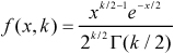, where k I and Γ(k/2) is the gamma function, which has closed-form values for half-integers (i.e., , where !! is the double factorial function). , where Γ(k/2) is the gamma function and γ(k / 2, x/2) is the lower incomplete gamma function , which does not have a closed form.

Statistics: Mean k, median ≈ k(1 − 2 / (9k))³, mode max(k − 2, 0), variance 2k.

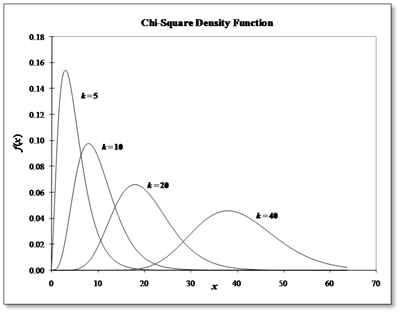
Graph: The graph below shows the chi-square density function for a range of k values.

Excel: Excel 2003/2007 uses CHIDIST(x, k) to return the one-tailed (right tail) probability of the chi-square distribution with k degrees of freedom, CHIINV(p, k) returns the inverse of the one-tailed (right tail) probability of the chisquare distribution, and CHITEST(actual_range, expected_range) can be used for the chi-square test. The chi-square density is not available in Excel, but the equivalent Excel function GAMMADIST(k/2, 2) can be used. Excel 2010 has the CHISQ.DIST(x, degrees_of_freedom, cumulative) and several other related functions.

Relationships to other distributions: The chi-square is a special case of the gamma distribution where χ²(k) = Γ(k / 2,2). The chi-square is the sum of k independent random variables; therefore, by the central limit theorem, it converges to the normal as k approaches infinity. The chi-square will be close to normal for k > 50 and will approach the standard normal.

See chi-square goodness of fit test, gamma distribution, gamma function, probability density function, probability distribution.

chi-square goodness of fit test – A statistical test used to determine if a set of data fits a hypothesized discrete probability distribution.

The chi-square test statistic is 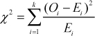, where O_i is the observed frequency in the i-th bin and E_i is the expected frequency. E_i is n(F(x_it) – F(x_ib)), where is the total number of observations, F(x) is the distribution function for the hypothesized distribution, and (x_ib, x_it) are the limits for bin i. It is important that every bin has at least five observations.

The hypothesis that the data follow the hypothesized distribution is rejected if the calculated χ² test statistic is greater than χ²_1-α,k-1, the chi-square distribution value with k - 1 degrees of freedom and significance level of α. The formula for this in Excel is CHIINV(1− α, k−1). The Excel function CHITEST(actual_range, expected_range) can also be used.

Failure to reject the null hypothesis of no difference should not be interpreted as “accepting the null hypothesis.” For smaller sample sizes, goodness-of-fit tests are not very powerful and will only detect major differences. On the other hand, for a larger sample size, these tests will almost always reject the null hypothesis because it is almost never exactly true. As Law and Kelton (2002) stated, “This is an unfortunate property of these tests, since it is usually sufficient to have a distribution that is ‘nearly’ correct.”

The Kolmogorov-Smirnov (KS) test is generally believed to be a better test for continuous distributions.

See Box-Jenkins forecasting, chi-square distribution, Kolmogorov-Smirnov test (KS test).

CIM – See Computer Integrated Manufacturing.

clean room – A work area where air quality, flow, flow direction, temperature, and humidity are carefully regulated to protect sensitive equipment and materials.

Clean rooms are frequently found in electronics, pharmaceutical, biopharmaceutical, medical device, and other manufacturing environments. Clean rooms are important features in the production of integrated circuits, hard drives, medical devices, and other high-tech and sterile products. The air in a clean room is repeatedly filtered to remove dust particles and other impurities.

The air in a typical office building contains from 500,000 to 1,000,000 particles (0.5 micron or larger) per cubic foot of air. A human hair is about 75-100 microns in diameter, but a particle that is 200 times smaller (0.5 micron) than a human hair can cause a major disaster in a clean room. Contamination can lead to expensive downtime and increased production cost. The billion-dollar NASA Hubble Space Telescope was damaged because of a particle smaller than 0.5 micron.

People are a major source of contamination. A motionless person produces about 100,000 particles of 0.3 micron and larger per minute. A person walking produces about 10 million particles per minute.

The measure of the air quality in a clean room is defined in Federal Standard 209E. A Class 10,000 clean room can have no more than 10,000 particles larger than 0.5 micron in any given cubic foot of air. A Class 1000 clean room can have no more than 1000 particles and a Class 100 clean room can have no more than 100 particles. Hard disk drive manufacturing, for example, requires a Class 100 clean room.

People who work in clean rooms must wear special protective clothing called bunny suits that do not give off lint particles and prevent human skin and hair particles from entering the room’s atmosphere.

click-and-mortar – A hybrid between a dot-com and a “brick-and-mortar” operation.

See dot-com.

clockspeed – The rate of new product introduction in an industry or firm.

High clockspeed industries, such as consumer electronics, often have product lifecycles of less than a year. In contrast, low clockspeed industries, such as industrial chemicals, may have product life cycles measured in decades. High clockspeed industries can be used to understand the dynamics of change that will, in the long run, affect all industries. The term was popularized in the book Clockspeed by Professor Charles Fine from the Sloan School at MIT (Fine 1995).

See New Product Development (NPD), time to market.

closed-loop MRP – An imprecise concept of a capacity feedback loop in a Materials Requirements Planning (MRP) system; sometimes called closed-loop planning.

Some consultants and MRP/ERP software vendors used to claim that their systems were “closed-loop” planning systems. Although they were never very precise in what this meant, they implied that their systems provided rapid feedback to managers on capacity/load imbalance problems. They also implied that their closedloop systems could somehow automatically fix the problems when the load exceeded the capacity. The reality is that almost no MRP systems automatically fix capacity/load imbalance problems. Advanced Planning and Scheduling (APS) Systems are designed to create schedules that do not violate capacity, but unfortunately, they are hard to implement and maintain.

See Advanced Planning and Scheduling (APS), Business Requirements Planning (BRP), capacity, Capacity Requirements Planning (CRP), finite scheduling, Materials Requirements Planning (MRP), Sales & Operations Planning (S&OP).

cloud computing – Internet-based computing that provides shared resources, such as servers, software, and data to users.

Cloud computing offers many advantages compared to a traditional approach where users have their own hardware and software. These advantages include (1) reduced cost, due to less investment in hardware and software and shared expense for maintaining hardware, software, and databases, (2) greater scalability, (3) ease of implementation, and (4) ease of maintainence.

Potential drawbacks of cloud computing include (1) greater security risk and (2) less ability to customize the application for specific business needs. Cloud computing includes three components: Cloud Infrastructure, Cloud Platforms, and Cloud Applications. Cloud computing is usually a subscription or pay-per-use service. Examples include Gmail for Business and salesforce.com.

See Application Service Provider (ASP), Software as a Service (SaaS).

cluster analysis – A method for creating groups of similar items.

Cluster analysis is an exploratory data analysis tool that sorts items (objects, cases) into groups (sets, clusters) so the similarity between the objects in a group is high and the similarity between groups is low. Each item is described by a set of measures (also called attributes, variables, or dimensions). The dissimilarity between two items is a function of these measures. Cluster analysis, therefore, can be used to discover structures in data without explaining why they exist.

For example, biologists have organized different species of living beings into clusters. In this taxonomy, man belongs to the primates, the mammals, the amniotes, the vertebrates, and the animals. The higher the level of aggregation, the less similar are the members in the respective class. For example, man has more in common with all other primates than with more “distant” members of the mammal family (e.g., dogs).

Unlike most exploratory data analysis tools, cluster analysis is not a statistical technique, but rather a collection of algorithms that put objects into clusters according to well-defined rules. Therefore, statistical testing is not possible with cluster analysis. The final number of clusters can be a user-input to the algorithm or can be based on a stopping rule. The final result is a set of clusters (groups) of relatively homogeneous items.

Cluster analysis has been applied to a wide variety of research problems and is a powerful tool whenever a large amount of information is available and the researcher has little prior knowledge of how to make sense out of it. Examples of cluster analysis include:

• Marketing research: Cluster consumers into market segments to better understand the relationships between different groups of consumers/potential customers. It is also widely used to group similar products to define product position.

• Location analysis: Cluster customers based on their locations.

• Quality management: Cluster problem causes based on their attributes.

• Cellular manufacturing: Cluster parts based on their routings.

A dendrogram is a graphical representation of the step-by-step clustering process. In the dendrogram on the right, the first step divides the entire group of items (set A) into four sets (B, C, D, E). The second step divides B into sets F and G, divides C into sets H and I, and divides E into sets J and K. In the last step, set G is divided into sets L and M, and set J is divided into sets N, O, and P. Therefore, the final clusters are on the bottom row (sets F, L, M, H, I, D, N, O, P, and K). Note that each of these final sets may include only one item or many items.

Dendrogram example

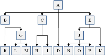
Source: Professor Arthur V. Hill

The distance between any two objects is a measure of the dissimilarity between them. Distance measures can be computed from the variables (attributes, dimensions) that describe each item. The simplest way to measure the distance between two items is with the Pythagorean distance. When we have just two variables (x_i, y_i) to describe each item i, the Pythagorean distance between points i and j is . With three variables (x_i, y_i, z_i) to describe each item, the Pythagorean distance is . With K variables, x_ik is defined as the measurement on the k-th variable for item i, and the Pythagorean distance between items i and j is defined as .

The Minkowski metric is a more generalized distance metric. If item i has K attributes (x_i1, x_i2, ... , x_iK), the distance between item i and item j is given by . The Minkowski metric is equal to the Euclidean distance when r = 2 and the Manhattan square distance when r = 1.

When two or more variables are used to define distance, the one with the larger magnitude tends to dominate. Therefore, it is common to first standardize all variables, i.e., , where is the sample mean for the k-th variable and s_k is the sample standard deviation. However, even with standardization, not all variables should have the same weight in the summation. Unfortunately, it is usually not clear how to determine how much weight should be given to each variable.

Many clustering algorithms are available. The objective functions include the complete-linkage (or farthest-neighbor), single-linkage (or nearest-neighbor), group-average, and Ward’s method. Ward’s method is one of the more commonly used methods and measures the distance (dissimilarity) between any two sets (S₁, S_j) as the sum of the squared distances between all pairs of items in the two sets, i.e., . Divisive methods start with all items in one cluster and then split (partition) the cases into smaller and smaller clusters. Agglomerative methods begin with each item treated as a separate cluster and then combine them into larger and larger clusters until all observations belong to one final cluster.

A scree plot is a graph used in cluster analysis (and also factor analysis) that plots the objective function value against the number of clusters to help determine the best number of clusters. The scree test involves finding the place on the graph where the objective function value appears to level off as the number of clusters (factors) increases. To the right of this point is only “scree.” Scree is a geological term referring to the loose rock and debris that collects on the lower part of a rocky slope.

SPSS offers three general approaches to cluster analysis:

• Hierarchical clustering – Users select the distance measure, select the linking method for forming clusters, and then determine how many clusters best suit the data.

• K-means clustering – Users specify the number of clusters in advance and the algorithm assigns items to the K clusters. K-means clustering is much less computer-intensive than hierarchical clustering and is therefore preferred when datasets are large (i.e., N > 1000).

• Two-step clustering – The algorithm creates pre-clusters, and then clusters the pre-clusters.

Exploratory data analysis often starts with a data matrix, where each row in an item (case, object) and each column is a variable that describes that item. Cluster analysis is a means of grouping the rows (items) that are similar. In contrast, factor analysis and principal component analysis are statistical techniques for grouping similar (highly correlated) variables to reduce the number of variables. In other words, cluster analysis groups items, whereas factor analysis and principal component analysis group variables.

See affinity diagram, algorithm, data mining, data warehouse, factor analysis, logistic regression, Manhattan square distance, Minkowski distance metric, Principal Component Analysis (PCA), Pythagorean Theorem.

CMM – See Capability Maturity Model

CNC – See Computer Numerical Control.

co-competition – See co-opetition.

COD – See Cash on Delivery (COD).

coefficient of determination – See correlation.

coefficient of variation – A measure of the variability relative to the mean, measured as the standard deviation divided by the mean.

The coefficient of variation is used as a measure of the variability relative to the mean. For a sample of data, with a sample standard deviation s and sample mean , the coefficient of variation is . The coefficient of variation has no unit of measure (i.e., it is a “unitless” quantity).

The coefficient of variation is often a good indicator of the distribution of the random variable. For example, c = 1 suggests an exponential distribution. More generally, the k parameter of a k-Erlang (or gamma) distribution is .

In forecasting, a good rule of thumb is that any item with a coefficient of variation of demand less than 1 has “lumpy” demand and therefore should not be forecasted with exponential smoothing methods.

See Croston’s Method, Erlang distribution, exponential distribution, exponential smoothing, forecasting, lumpy demand, standard deviation.

Collaborative Planning Forecasting and Replenishment (CPFR) – A business practice that combines the intelligence of multiple trading partners in the planning and fulfillment of customer demand (source: www.vics.org/committees/cpfr, April 16, 2011).

CPFR is designed to improve the flow of goods from the raw material suppliers to the manufacturer and ultimately to the retailers’ shelves. It is also designed to quickly identify any discrepancies in the forecasts, inventory, and ordering data so the problems can be corrected before they impact sales or profits.

With CPRF, customers share their sales history, sales projections, and other important information with their business partners, who, in turn, share their raw material availability, leadtimes, and other important information with the customers. The information is then integrated, synchronized, and used to eliminate excess inventory and improve in-stock positions, making the supply chain more profitable.

CPFR has data and process model standards developed for collaboration between suppliers and an enterprise with methods for planning (agreement between the trading partners to conduct business in a certain way), forecasting (agreed-to methods, technology and timing for sales, promotions, and order forecasting), and replenishment (order generation and order fulfillment). The Voluntary Inter-Industry Commerce Standards (VICS) committee, a group dedicated to the adoption of barcoding and EDI in the department store/mass merchandise industries, has established CPFR standards for the consumer goods industry that are published by the Uniform Code Council (UCC). See www.vics.org for information on the VICS committee.

See continuous replenishment planning, Efficient Consumer Response (ECR), forecasting.

Collaborative Product Development – See Early Supplier Involvement, New Product Development (NPD).

co-location – The practice of locating people from different functions or different organizations next to each other to improve communications.

Co-location has proven to be very helpful for both customers and suppliers when suppliers have representatives working at their customers’ sites. For example, many manufacturers have representatives working in Bentonville, Arkansas, at Walmart’s world headquarters.

Co-location makes sense for many large and complex organizations to co-locate workers from different functions to improve communications. For example, Tom Ensign, formerly the business unit manager for 3M Post-it Products, reported that one of his keys to success was the co-location of his office next to his marketing and manufacturing directors. Co-location also makes sense for project teams working on larger projects.

See JIT II, learning organization, project management, vendor managed inventory (VMI).

combinations – The number of ways that n items can be grouped in sets of r items without regard to order; also called the binomial coefficient.

In probability and statistics, analysts often need to know the number of ways that it is possible to arrange n things into groups of r items. The number of unique combinations of n things taken r at a time is . Note that the number of combinations is symmetric, i.e., C(n, r) = C(n, n – r). See the factorial entry for the definition of n! For example, a deck of playing cards has 52 cards. In the game of Bridge, each player has a hand of 13 cards. The number of possible combinations (hands) for a Bridge player, therefore, is “52 taken 13 at a time,” which is . Order does not matter with combinations. The Excel function for combinations is COMBIN(n, r).

In constrast, a unique ordering (sequence) of a set of items is called a permutation. The number of unique ways that a set of n items can be ordered is called the number of permutations and is written mathematically as n! and read as “n-factorial.” For example, the set {1,2,3} has 3! = 3·2·1 = 6 permutations: {1,2,3}, {1,3,2}, {2,1,3}, {2,3,1}, {3,1,2}, and {3,2,1}. A 13-card Bridge hand can be arranged in 13! = 6,227,020,800 different ways. The Excel function for n! is FACT(n).

For both combinations and permulations, most computers will have overflow issues when n 171. See the gamma function entry for suggestions for handling these issues.

See binomial distribution, factorial, gamma function.

commercialization – The process of managing a new product through pilot production, production ramp-up, and product launch into the channels of distribution.

See New Product Development (NPD).

committee – A group of people who work to provide a service for a larger organization.

Committees consist of people who volunteer or are appointed. Although many sources use the terms committee and project team interchangeably, the project management literature considers a committee to be an on-going organizational structure and a project team to be a temporary organizational structure that disbands when the task is complete. A standing committee serves an on-going function, whereas an ad hoc committee is a project team with a limited duration. The Latin phrase “ad hoc” means “for this purpose” and indicates an improvised or impromptu team assigned to fill a particular need.

See project management.

commodity – (1) Inventory management: A standard product that is homogenous and cannot be easily differentiated by suppliers (e.g., salt). (2) Purchasing management: A group of similar products often managed by a single buyer (e.g., electronic components).

In the inventory management context, all suppliers offer essentially the same good or product, which means that commodity products from two or more suppliers are essentially interchangeable and uniform. As a result, the main differentiator for commodities is the supplier’s price. Common examples of commodities include basic resources (e.g., oil and coal) and agricultural products (e.g., wheat and corn). Many commodities are traded on an exchange and many well-established commodities have actively traded spot and derivative markets. In some cases, minimum commodity quality standards (known as a basis grade) are set by the exchange.

Suppliers often try to differentiate commodity products with packaging, quality, information, service, and delivery. However, in many cases, customers only care about the price. It is often important for sellers to ensure that their products continue to be differentiated so their products are not treated like a commodity and purchased only on the basis of price.

Many industries have found that highly differentiated products can become less differentiated and even commoditized over time. For example, simple handheld calculators were once a highly differentiated luxury item costing hundreds of dollars⁸. Today, they are fairly undifferentiated, sell for under $20, and are essentially a commodity product.

In the purchasing context, the word “commodity” is used to mean any group of purchased materials or components, also known as a commodity class. In this context, a commodity can be any group of purchased items, including highly engineered items. For example, Boston Scientific might have a manager for a commodity group that includes all machined products.

See category management, futures contract, purchasing, single source, sourcing, standard parts.

common carrier – An organization that transports people or goods and offers its services to the public, typically on regular routes and regular schedules.

In contrast, private carriers do not provide service to the public and provide transport on an irregular or ad hoc basis. Examples of common carriers include airlines, railroads, bus lines, cruise ships, and many trucking companies. Although common carriers generally transport people or goods, the term may also refer to telecommunications providers and public utilities in the U.S.

A common carrier must obtain a certificate of public convenience and necessity from the Federal Trade Commission for interstate traffic. A common carrier is generally liable for all losses that may occur to property entrusted to its charge in the course of business, with four exceptions: (1) an act of God, (2) an act of public enemies, (3) fault or fraud by the shipper, or (4) an inherent defect in the goods. Carriers typically incorporate further exceptions into a contract of carriage, often specifically claiming not to be a common carrier.

See carrier, for-hire carrier, logistics, private carrier.

common cause variation – A statistical process control term for natural or random variation that is inherent in a process over time and affects the process at all times.

Common cause variation includes the normal, everyday influences on a process. If a process is in control, it only has common cause variation. This type of variation is hard to reduce because it requires change to the fundamental process. Pande et al. (2000) referred to problems from common causes as “chronic pain.” Special cause variation is the alternative to common cause variation.

See Capability Maturity Model (CMM), control chart, process capability and performance, quality management, special cause variation, Statistical Process Control (SPC), Statistical Quality Control (SQC), tampering, tolerance.

commonality – The degree to which the same parts are used in different products.

In the photo below, the “universal” box in the front middle replaces all the other boxes in the back. The change to this common box dramatically reduced inventory and manufacturing cost. (This photo is used with permission from Honeywell.) Honeywell calls this a “universal” box. These types of components are also called robust components. In general, robust components have higher direct labor cost because they have better product design quality. However, increasing commonality can lead to economies of scope in many ways:

• Reduced setup (ordering) cost – Because the robust component has a higher demand rate, its economic order quantity is larger and it does not have to be ordered as many times as the current components. This saves on ordering cost.

Example of commonality

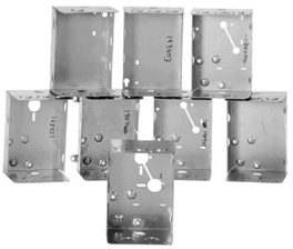
• Potential quantity discounts for materials – However, robust components have higher demand and therefore can qualify for a quantity discount on the price.

• Reduced cycle (lotsize) inventory – The economic order quantity logic suggests that robust components have a larger order size than any of the current components. However, the total cycle stock for the robust component will be less than the sum of the cycle stock for the two current components. This will result in lower carrying cost.

• Reduced safety stock inventory and improved service levels – The variance of the demand during leadtime for a robust component is likely about equal to the sum of the variance of the demand for the two current components. When this is true, the robust component requires less safety stock inventory. Conversely, the firm can keep the same safety stock level and improve the service level or make improvements in both. This can result in lower carrying cost, lower stockout cost, or both.

• Reduced forecasting error – Based on the same logic as above, the robust component has lower forecast error variance than the sum of the variances of the two current components. Again, this can reduce safety stock inventory, improve service levels, or both.

• Reduced product design cost – If the firm is using truly robust components, it can use these components in different products and not have to “reinvent the wheel” with each new product design.

• Reduced purchasing and manufacturing overhead – As the number of components are reduced, the overhead needed to maintain the engineering drawings, tooling, etc. can also be reduced.

• Increased reliability – In some cases, a more robust part is also more reliable and easier to maintain.

Commonality is closely related to the concepts of standard parts and interchangeable parts.

See agile manufacturing, bill of material (BOM), cycle stock, economy of scale, economy of scope, engineer to order (ETO), interchangeable parts, interoperability, mass customization, modular design (modularity), overhead, quantity discount, reliability, robust, service level, standard parts, standard products, value engineering.

competitive analysis – A methodology used to help an organization identify its most important current and future competitors, analyze how these competitors have positioned their products and services in the market, evaluate these competitors’ strengths and weaknesses, and then develop strategies to gain competitive advantage in the market.

See five forces analysis, industry analysis, operations strategy, SWOT analysis.

Compounded Annual Growth Rate (CAGR) – The rate of growth for an investment that assumes that the compounded growth rate per period is constant between the first and last values; also called the internal rate of return (IRR) and smoothed rate of return.

The CAGR (pronounced “keg-er”) is also called a smoothed rate of return because it measures the growth of an investment as if it had grown at a steady rate on an annually compounded basis. Mathematically, the CAGR is the geometric mean growth rate and is computed as , where n is the number of periods (usually years). For example, if someone made an initial investment worth $10,000 at the end of 2007, $11,000 at the end of 2008, $12,000 at the end of 2009, and $19,500 at the end of 2010, the Compounded Annual Growth Rate (CAGR) over this n = 3 year period is (19,500/10,000)^1/3 − 1 = 24.9%. In other words, if the growth rate over the three years was constant each year, it would be an annual growth rate of 24.9%. To prove this, we can see that $10,000 × 1.249 × 1.249 × 1.249 = $19,500. Note that this example has balances for four years (2007, 2008, 2009, and 2010), but only three years for computing growth. In summary, the CAGR is not the average (arithmetic mean) annual return but rather the geometric mean annual return.

The Excel functions IRR(values_range) and XIRR(values_range, dates_range) can be used to calculate the CAGR. IRR is for periodic returns and XIRR allows the user to define a schedule of cash flows. Both functions require at least one positive and one negative value. If this function is not available in Excel and returns the #NAME? error, install and load the Analysis ToolPak add-in.

See financial performance metrics, geometric mean, Internal Rate of Return (IRR).

Computer Aided Design (CAD) – A combination of hardware and software that enables engineers and architects to design everything from furniture to airplanes.

In addition to the software, CAD systems usually require a high-quality graphics monitor, mouse, light pen, or digitizing tablet for drawing, and a special printer or plotter for printing design specifications. CAD systems allow an engineer to view a design from any angle and to zoom in or out for close-ups and long-distance views. In addition, the computer keeps track of design dependencies so that when the engineer changes one value, all other values that depend on it are automatically changed. Until the mid-1980s, CAD systems were specially constructed computers. Today, CAD software runs on general-purpose workstations and personal computers.

See Computer Aided Design/Computer Aided Manufacturing (CAD/CAM), Computer Numerical Control (CNC), group technology, New Product Development (NPD).

Computer Aided Design/Computer Aided Manufacturing (CAD/CAM) – Computer systems used to design and manufacture products.

An engineer can use the system to design a product and generate the instructions that can be used to control a manufacturing process.

See Computer Aided Design (CAD).

Computer Aided Inspection (CAI) – A system for performing inspection through the use of computer hardware and software technologies.

CAI tools are categorized as either contact or non-contact methods:

Contact methods – Coordinate Measuring Machines (CMMs) use a Computer Numerically Controlled (CNC) mechanical probe to inspect parts to an accuracy of as little as 0.0002 inch. However, the CMM probe may damage or deform a product’s surface and are not appropriate when contamination is a concern. With many sample points or complex product contours, CMMs may be too slow to support the desired product inspection rate. Contact methods are slower but cost less than non-contact methods.

Non-contact methods/Vision systems – A camera is used to take a video image of a part. The image is processed by software and electronic hardware to compare it against a reference template. The vision system determines the placement, size, and shape of holes and the presence of part features.

Non-contact methods/Laser-scan micrometers – These systems use reflected laser light to measure part dimensions and are used to inspect single dimensions on highly repetitive work, such as intervals, diameters, widths, heights, and linearity.

See inspection, Statistical Process Control (SPC).

Computer Aided Manufacturing (CAM) – See Computer Aided Design (CAD), Computer Aided Design/Computer Aided Manufacturing (CAD/CAM), Computer Numerical Control (CNC).

Computer Based Training (CBT) – Self-paced instruction via interactive software; sometimes called Computer Based Instruction (CBI), e-learning, and distance education.

CBT provides an opportunity for individuals to learn a subject with little or no involvement of an instructor. Content can include videos, quizzes, tests, simulations, and “hands-on” learning by doing in a “virtual world.”

See cross-training.

Computer Integrated Manufacturing (CIM) – See Computer Aided Design (CAD), Computer Aided Design/Computer Aided Manufacturing (CAD/CAM), Computer Numerical Control (CNC).

Computer Numerical Control (CNC) – A type of controller that is typically found on machining centers and other machine tools.

CNC machines typically cut and form metal. A CNC includes a machine tool used to turn, drill, or grind different types of parts and a computer that controls the sequence of processes performed by the machine. Not all computer-controlled machines are CNC. For example, robots are not considered to be CNC machines.

See Computer Aided Design (CAD), manufacturing processes.

computer simulation – See simulation.

concurrent engineering – A systematic approach to the integrated, simultaneous design of products and their related processes, including manufacturing and support; also called simultaneous engineering and Integrated Product Development (IPD).

The goal of current engineering is to reduce time to market and quality problems. It can accomplish these goals by engaging appropriate cross-functional teams from engineering, operations, accounting, procurement, quality, marketing, and other functions. Suppliers are also involved in some cases.

See cross-functional team, Early Supplier Involvement (ESI), Integrated Product Development (IPD), New Product Development (NPD), Quality Function Deployment (QFD), simultaneous engineering, waterfall scheduling.

conference room pilot – See pilot test.

confidence interval – A range of values that will contain the true mean for a random variable with a user-specified level of confidence based on a given sample of data.

Given a set of n > 30 random observations on a random variable, the confidence interval on the true mean is given by , where is the sample mean, s is the sample standard deviation, and z_a/2 = F^-1 (1 - a/2) is the z value associated with probability α/2. If n random samples are taken many times, this interval will “capture” the true mean about 100·α/2 percent of the time. The procedure is as follows:

Step 0. Define the parameters – Specify the number of observations (n) that have been collected, the estimated size of the population (N), and the confidence level parameter (α). If the size of N is large but unknown, use an extremely large number (e.g., N = 10¹⁰).

Step 1. Compute the sample mean and standard deviation – Compute the sample mean and sample standard deviation s from the n observations.

Step 2. Find the z or t value – When n < 30, use the, t_α/2,n-1 value from a Student’s t table or the Excel statement TINV(α, n −1). Note: The arguments in this Excel function are correct. The Excel functions TINV and NORMSINV are inconsistent in how they handle the probability parameter (α). TINV returns the probability associated with the two-tailed Student’s t-distribution. When n 30, use the z_α/2 value from a normal table or the Excel statement NORMSINV(1 − α/2).

Step 3. Compute the half-width – Compute the half-width of the confidence interval using (replace z_α/2 with t_{α/2,n - 1} when n < 30). If the sample size n is large relative to the total population N (i.e., n/N > 0.05), use instead. The term is called the finite population correction factor. For n 30, the half-width can also be found using the Excel function CONFIDENCE(α, s, n). This Excel function should not be used when n < 30.

Step 4. Write the confidence interval – Write the 100(1 − α)% confidence interval as .

Confidence intervals are a useful concept based on the central limit theorem and do not require any assumptions about the distribution of x. The sample size calculation entry has more detail on this subject.

See Analysis of Variance (ANOVA), central limit theorem, Chebyshev’s inequality, dollar unit sampling, normal distribution, sample size calculation, sampling, sampling distribution, simulation, standard deviation, Student’s t distribution, t-test.

configuration control – See configuration management.

configuration management – The process of defining and controlling the information that defines a system.

Configuration control includes all activities needed to control the changes to a configuration after it has been formally documented. Configuration control includes the evaluation, coordination, approval, or rejection of changes.

The best configuration management process is one that can (1) accommodate change, (2) accommodate reuse of proven standards and best practices, (3) assure that all requirements remain clear, concise, and valid, (4) communicate promptly and precisely, and (5) assure that the results conform in each case. CM includes several elements: requirements management, change management, release management, data management, records management, document control, and library management. CM provides the infrastructure that enables an organization to “change faster and document better.” CM also accommodates change and keeps requirements clear, concise, valid, and synchronized. A strong CM process is the foundation of a sound business process infrastructure. Adapted from the home page of the Institute of Configuration Management (www.icmhq.com).

See New Product Development (NPD).

configurator – A software tool (usually with an Internet interface) that allows customers, order entry people, or sales people to create customized products by selecting various product features from menus.

Ideally, a configurator will (1) encourage customers to select standard, high-margin combinations of features, (2) prevent customers from selecting prohibitive combinations of features, (3) discourage customers from selecting low margin (or negative margin) combinations, and (4) create manufacturing orders that can be sent electronically to manufacturing. In some cases, the configurator creates instructions for automated equipment. Configurators might contain many expert rules and might draw heavily on science, engineering, and manufacturing expertise. In conclusion, the ideal configurator is easy for the customer to use, creates product configurations that customers want, and guides customers to product configurations that the firm can make and sell profitably.

For example, mycereal.com⁹, General Mills’ custom-blended breakfast cereal, had a configurator that included tremendous amounts of food science so customers would get healthy food and tasty portions. Lifetouch provides software to high schools so they can configure their own student ID cards, populate a database with student photos, and then send a file to the firm’s ID card manufacturing facility.

See configure to order (CTO), engineer to order (ETO), mass customization, order entry.

configure to order (CTO) – A customer interface strategy that adjusts parameters or adds modules to a product in response to a customer’s order.

In a configure to order (CTO) system, a firm sells standard products that require parameter adjustments or modules to be added in response to a customer order. Examples include setting the height of a seat for a riding mower, selecting the language option for a software package, or setting some customer-specific parameters for a medical device. Some people call this reconfigure to order. The respond to order (RTO) entry discusses a number of similar customer interface strategies.

See configurator, respond to order (RTO), standard products.

conformance quality – The degree to which the product or service meets the design specifications or standards; sometimes also called quality of the process or process quality.

Conformance quality is generally measured by the yield rate (the percentage of units started that are not defective) or the scrap rate (the percentage of units started that have to be discarded because they are defective). In contrast, design quality (also called performance quality) is the degree to which the design meets customer requirements.

For example, the new product development organization has set a performance standard (a specification limit) that a new wristwatch should be able to survive in 100 meters of water. However, the manufacturing process sometimes fails to properly assemble the watch, which results in 10% of all watches failing to meet the standard. In this example, the yield rate is 90% and the percent defective is 10%.

See product design quality, quality at the source, quality management, scrap, yield.

congestion pricing – The practice of charging a higher price for a service during peak demand periods to discourage arrivals to the system.

For example, the city of Singapore assesses a very high charge to drivers who enter the downtown areas during the workday. This practice is now being used in many large metropolitan areas worldwide. Similar examples can be found in telephone rates, electricity (power) usage, computer usage, restaurants, and other service businesses.

See yield management.

conjoint analysis – An analytical marketing research technique that measures the trade-offs made by respondents among product attributes.

Conjoint analysis is a useful tool for both product concept generation and evaluation by rating product attributes in terms of their importance in the market. The method involves the measurement of the collective effects of two or more independent variables (e.g., color, size, ease of use, cost, etc.) on the classification of a dependent variable (overall liking, purchase intention, best buy, or any other evaluative measurement). The stimulus is a product-attribute combination. Various mixed and matched product attributes are put together and rated by the respondent. For example, does the respondent prefer a large, powerful, spacious car that is relatively expensive in its operation or one that is smaller, less powerful, but more economic to operate?

Once the unique product combinations are established, conjoint studies typically collect data via the use of one of the following:

• A paired-comparison methodology, where each of the hypothetical products is directly compared to another product and one of the products is selected over the other. For example, with 16 unique products, a total of 120 binary choices are required.

• A ranking methodology, where product configurations are rank-ordered relative to preferences of the respondent. This is probably the most common method for collecting conjoint data.

For the paired-comparisons model, a telephone survey is often difficult because of the amount of time required to go through each of the possible comparisons.

Adapted from http://mrainc.com/trad_conj.html (April 16, 2011).

See Analytic Hierarchy Process (AHP).

consignee – A transportation term for the party (agent) that accepts a delivery.

The consignee is named on the bill of lading as the party authorized to take delivery of a shipment.

See Advanced Shipping Notification (ASN), bill of lading, consignment inventory.

consignment inventory – Items in the possession of a retailer or distributor and offered for sale to customers but still owned by the supplier.

Consignment inventory is often used as a marketing tool to entice a retailer or distributor to carry a supplier’s inventory. Payment on consignment inventory is usually made when stock is sold or used by a customer. The supplier (the consignor) ships to the agent (the consignee) under an agreement to sell the goods for the consignor. The consignor retains title to the goods until the consignee has sold them. The consignee sells the goods and then pays a commission to the consignor.

Some examples of consignment inventory include: (1) Many retailers of Christmas craft items only pay their suppliers when the craft items are sold. (2) Medical device firms often own the devices in hospital inventories until they are sold to patients. (3) Some manufacturers of fasteners make their products available to assemblers and do not require their customers to pay until the fasteners are used.

See consignee, inventory management, vendor managed inventory (VMI).

consolidation – (1) In a general context: The combination of separate parts into a single unified whole. (2) In a logistics context: The combination of two or more shipments going to the same destination in a single shipment; related terms include consolidate, consolidation service, freight consolidation, consolidated shipment, consolidated cargo, consolidated load, and consolidated container.

A consolidated shipment can reduce the number of individual shipments and take advantage of lower cost transportation (i.e., full truck or full container load shipments). At the destination, the consolidated shipment is separated (de-consolidated or de-grouped) back into the original individual shipments for delivery to consignees. A consolidation service will combine smaller shipments and then ship them together to achieve better freight rates and cargo security.

Consolidation is also used in the context of reducing the number of stocking locations (e.g., warehouses) and consolidating the “spend” on just a few suppliers for each commodity group (e.g., MRO supplies).

See cross-docking, hub-and-spoke system, less than truck load (LTL), leverage the spend, Maintenance-Repair-Operations (MRO), pooling, square root law for warehouses, Third Party Logistics (3PL) provider.

consortium – An association or coalition of two or more individuals, companies, firms, or not-for-profit organizations (or any combination thereof) that pool resources, such as buying power, research capability, manufacturing capability, libraries, or information, to achieve a common goal.

Constant WIP – See CONWIP.

constraints management – See Theory of Constraints.

consumable goods – An item or product that is used up (consumed) in a relatively short period of time; sometimes called non-durable goods, soft goods, or consumables.

In the economics literature, consumable goods are defined as products that are used up fairly quickly and therefore have to be replaced frequently. In contrast, durable goods (also called hard goods or capital goods), such as refrigerators, cars, furniture, and houses, have long useful lives.

In the Maintenance, Repair, and Operations (MRO) context, consumables are items purchased by a firm that do not become part of the product sold to customers. For example, 3M sandpaper might be used for final surface conditioning of a product. Other examples of consumables include printer ink and machine oil.

In a marketing context, many firms make more money selling consumable products than they do selling capital goods or other products. For example, Gillette almost gives away its razors to sell razor blades and HP sells printers with lower margins than it has on its ink cartridges.

See category captain, category management, consumer packaged goods, durable goods, Maintenance-Repair-Operations (MRO).

consumer packaged goods – Consumable goods, such as food and beverages, footwear and apparel, tobacco, and cleaning products; sometimes abbreviated CPG.

Some examples of consumer packaged goods include breakfast cereal (such as General Mill’s Cheerios) and soap (such as Proctor and Gamble’s Ivory soap).

See category captain, category management, consumable goods, Fast Moving Consumer Goods (FMCG), private label, trade promotion allowance.

consumer’s risk – The probability of accepting a lot that should have been rejected.

More formally, consumer’s risk is the probability of accepting a lot with a defect level equal to the Lot Tolerance Percent Defective (LTPD) for a given sampling plan. The consumer suffers when this occurs because a lot with unacceptable quality was accepted. This is called a Type II error. The symbol β is commonly used for the Type II risk.

See Acceptable Quality Level (AQL), acceptance sampling, Lot Tolerance Percent Defective (LTPD), operating characteristic curve, producer’s risk, quality management, sampling, Type I and II errors.

container – See shipping container.

continuous demand – See demand.

continuous flow – Producing and moving small batches (ideally with a lotsize of one unit) through a series of processing steps with almost no inventory and almost no waiting between steps.

See batch-and-queue, discrete manufacturing, facility layout, lean thinking, one-piece flow, repetitive manufacturing.

continuous improvement – See kaizen, lean sigma, lean thinking, Total Quality Management (TQM).

continuous probability distribution – See probability density function.

continuous process – A process that makes only one product with dedicated equipment and never needs to handle changeovers (setups).

Examples of a continuous process include oil refining, paper making, and chemical processing.

See batch process, discrete manufacturing, setup cost, setup time.

continuous replenishment planning – The practice of working with distribution channel members to change from distributor-generated purchase orders to replenishment based on actual sales and forecast data.

The principal goal of continuous replenishment planning is to reduce the cost of producing and moving product through the vendor-retailer supply chain. The object is for all stages of the supply chain to operate with greater knowledge of downstream inventory conditions, thereby allowing for a synchronized flow of product from the manufacturer through point-of-sale (Vergin and Barr 1999).

See Collaborative Planning Forecasting and Replenishment (CPFR), Efficient Consumer Response (ECR), inventory management.

continuous review system – A system for managing an inventory that compares the inventory position (on-hand plus on-order less allocated) with the reorder point for every transaction and places a replenishment order when the position is less than the reorder point.

See inventory management, inventory position, periodic review system, reorder point, replenishment order.

Contract Electronics Manufacturing Services (CEMS) – See contract manufacturer.

contract manufacturer – An organization that makes products under a legal agreement with the customer.

Contract manufacturers generally serve the Original Equipment Manufacturing (OEM) market. Contract manufacturers make a large percentage of the products in the computer and electronics fields. These products are usually designed and branded with the OEM’s name, built by the contract manufacturer, and then shipped directly to distributors or customers.

A good example is the Microsoft Xbox game console, which is made by Flextronics and other contract manufacturers around the world. Flextronics also makes cell phones for Ericsson, routers for Cisco, and printers for HP. Other major contract electronics manufacturers include Sanmina-SCI Corporation and Celestica.

An “original design manufacturer” (ODM) is a type of contract manufacturer that uses its own designs and intellectual property (IP). The ODM typically owns the IP for the product itself, while the regular contract manufacturer uses its customer’s designs and IP. Whereas, contract manufacturers can make hundreds or thousands of different products, ODMs usually specialize in only a handful of categories. Contract manufacturers in the electronics field that not only make products but also offer assistance with the design and supply chain generally call themselves Electronics Manufacturing Services (EMS) or Contract Electronics Manufacturing Services (CEMS).

Porter (2000) listed the most prevalent sources of friction in a contract manufacturing relationship as:

• Traditional financial metrics.

• Difficulty defining core competencies.

• Fear of losing intellectual capital and expertise.

• Difficulty finding qualified manufacturing-services companies.

• Difficulty attracting good contract manufacturers for less-desirable programs.

• Difficulty understanding and documenting capabilities of contract manufacturers.

• Difficulty earning most-favored-customer status.

• Necessity of managing risk exposure.

• Trouble with technology and knowledge transfer.

• Unforeseeable problems (such as parts shortages).

See business process outsourcing, co-packer, intellectual property (IP), Original Equipment Manufacturer (OEM), outsourcing, supply chain management.

contract warehouse – See warehouse.

control chart – A graphical tool used to plot the statistics from samples of a process over time and keep the system in control.

If all points are within the upper and lower statistical control limits, variation may be ascribed to “common causes” and the process is said to be “in control.” If points fall outside the limits, it is an indication that “special causes” of variation are occurring and the process is said to be “out of control.” Eliminating the special causes first and then reducing common causes can improve quality. Control charts are based on the work of Shewhart (1939). The most commonly used control charts are the run chart, x-bar chart, r-chart, c-chart, and p-chart. Less commonly used control charts include the s-chart, s²-chart, u-chart, and np-chart.

See c-chart, common cause variation, cumulative sum control chart, lean sigma, np-chart, outlier, p-chart, process capability and performance, quality management, r-chart, run chart, seven tools of quality, special cause variation, specification limits, Statistical Process Control (SPC), Statistical Quality Control (SQC), tampering, u-chart, x-bar chart.

control limit – See Statistical Process Control.

control plan – A formal document that defines how an organization will continue to benefit from an organizational intervention, such as a lean sigma project.

When a process improvement project has been completed, it is important that the organization “sustain the gains.” This is often difficult given the normal organizational “entropy,” where the system tends to fall back into the old state of disorder. A good control plan includes the following elements:

• Procedure – What solutions were implemented to attain the project goals? What control device is in place?

• Responsible party – Who is responsible for this? See the RACI Matrix entry for a methodology.

• Nature of control – How does the control measure sustain the gain? What is the control measure for early detection?

• What to check – What does the responsible party inspect/observe? What are the failure modes?

• Action/Reaction – What does the responsible party do if the situation is out of control?

If statistical process control is appropriate, the following data items should be specified for each Key Process Output Variable (KPOV): Target value, lower specification limit, upper specification limit, C_pk, and the measurement system used to collect the data.

Good control plans go beyond statistical process control and include clear job descriptions, aligned reward systems, standard operating procedures, visual signals and instructions, and error proofing.

See ADKAR Model for Change, lean sigma, Lewin/Schein Theory of Change, RACI Matrix.

CONWIP – An approach for manufacturing planning and control that maintains a constant work-in-process inventory in the system.

With CONWIP (Spearman, Hopp, & Woodruff 1989), every time the last step in the process completes one unit, the first step in the process is given permission to start one unit. As a result, CONWIP maintains a constant WIP inventory. This is similar to the Theory of Constraints “drum buffer rope” (DBR) concept, except that CONWIP does not send a signal from the bottleneck, but rather sends the signal from the final step in the process. This concept is similar to a JIT pull system, except that CONWIP does not need to have buffers (kanbans) between each pair of workcenters. Given that CONWIP does not require the firm to identify the bottleneck and does not need to implement any type of kanban system between workcenters, it is clearly easier to operate than many other systems. CONWIP can be implemented with a simple visual control system that has the final operation signal the first operation every time a unit is completed. CONWIP can be applied at almost any level: at a machine, a workcenter, a plant, or even an entire supply chain. Some research suggests that CONWIP is superior to both DBR and JIT in terms of system performance (inventory, capacity, etc.).

See blocking, Drum-Buffer-Rope (DBR), gateway workcenter, kanban, pacemaker, POLCA (Paired-cell Overlapping Loops of Cards with Authorization), pull system, Theory of Constraints (TOC), Work-in-Process (WIP) inventory.

co-opetition – A blending of the words “cooperation” and “competition” to suggest that competing firms can sometimes work together for mutual benefit; also called co-competition and coopetition.

Cooperation with suppliers, customers, and firms producing complementary or related products can lead to expansion of the market and the formation of new business relationships, perhaps even the creation of new forms of business. An example can be found in group buying, where multiple, normally competitive, buying group members (such as hospitals) leverage the buying power of the group to gain reduced prices. All members of the buying group benefit from this relationship.

This concept was developed in the book Co-opetition (Brandenburger & Nalebuff 1996). Apparently, Ray Noorda, the founder of Novell, coined the term. The concept and term have been widely used in the computer industry, where strategic alliances are commonly used to develop new products and markets, particularly between software and hardware firms. Some industry observers have suggested that Apple and Microsoft need each other and, in fact, are involved in co-opetition.

Do not confuse this term with the term “co-opt,” which means to select a potential adversary to join a team.

See game theory.

co-opt – To appoint, select, or elect someone to become a member of a group, team, or committee, often for the purpose of neutralizing or winning over potential critics or opponents; also spelled coopt, co-option, and cooptation.

According to the Merriam-Webster Dictionary, co-opt comes from the Latin word “cooptare,” which means to choose. When selecting members for a project team, it is often wise to co-opt potential opponents. Ideally, this potential opponent becomes an advocate and recruits support from other like-minded potential opponents.

This term should not be confused with the term “co-opetition,” which is a cooperative relationship between competing firms.

See change management, project management, stakeholder analysis.

coordinate the supply chain – See buy-back contract.

co-packer – A supplier that produces goods under the customer’s brand; also copacker.

A co-packer is a contract manufacturer that produces and packs items for another company. The term “copacker” is frequently used in a consumer packaged goods context, but is also used in other industries. For example, Ecolab, a manufacturer of industrial cleaning products, uses co-packers to manufacture some cleaning agents that require specialized chemical processes and Schwan’s Foods uses co-packers when it does not have enough capacity, particularly for seasonal products.

See contract manufacturer, outsourcing.

core capabilities – See core competence.

core competence – Skills that enable an organization to differentiate its products and services from its competitors; nearly synonymous with distinctive competence.

Coyne, Hall, and Clifford (1997) defined a core competence as “a combination of complementary skills and knowledge bases embedded in a group or team that results in the ability to execute one or more critical processes to a world-class standard.” This definition is similar but not identical to the above definition. Nearly all definitions of core competence include the point that a core competence is an attribute of the organization and not just an attribute of a single individual in that organization.

A core competence is unique and hard to copy, which means that it can lead the firm into new products and markets. Some authors make a distinction between core competencies and distinctive competence. They define core competence as the basic product and process technologies and skills that all firms need to compete in an industry and distinctive competence as the set of technologies and skills that a firm uses to differentiate itself in the market. However, it appears that many authors now use the terms almost synonymously. Knowledge of a firm’s core competence can lead its management team to find new products and guide its thinking about outsourcing.

Many marketing experts and students tend to define a core competence as a differentiated product. However, a core competence is not a product or service, but rather the processes, abilities, and unique attributes (differentiated processes) that allow the organization to develop and deliver differentiated “core products.”

Three requirements for a valid distinctive competence are:

• It must be unique and present a barrier to entry for new competitors.

• The unique competence must offer real value to the marketplace. Something being merely unique without offering value is not a distinctive competence.

• The unique competence must be credible in the marketplace. Its existence and value have to be accepted and believed.

A popular phrase in many MBA classrooms is “An organization should never outsource its core competence.” With that said, it is interesting to see how many firms find that they are outsourcing today what they defined as their core competences less than five years ago. It may just be that core competences, like strategies, tend to change and adapt over time as the markets, products, and technologies change. Clearly, an organization’s set of core competences should not remain stagnant in a rapidly changing environment.

In this author’s experience, most executives cannot clearly identify their core competences when asked. However, one insightful way to help an organization identify its core competence is to ask, “What would keep a competitor from capturing 100% of your market share tomorrow?” This “barriers-to-entry” question usually identifies the organization’s core competence. Barriers to entry can include:

• Proprietary product or process technology

• Product differentiation (often based on process differentiation)

• Economies of scale (that lead to a lower cost structure)

• Brand equity

• Switching cost

• Government protection, subsidies, and patents

• Access to raw materials (special relationship or location)

• Access to customers (good location)

Another good question used to identify a core competence is, “Why do customers buy your product instead of another product?” This is the customer’s view of core competence.

Zook (2004) emphasizes the need for firms to stay close to their core products and core competence. His book offers a systematic approach for choosing among a range of possible “adjacency moves,” while always staying close to the core products and core competencies.

See economy of scale, focused factory, market share, operations strategy, outsourcing, resource based view, switching cost.

corporate portal – A Web-based system that allows businesses to make internal (IS/IT) systems or information available in a single location and format.

A portal is a Web site intended to be the first place people see when using the Web. Most portals have a catalog of web sites, a search engine, or both. Portals may also offer e-mail and other services to entice people to use that site as their main point of entry (hence “portal”). Portals are often used to allow access to internal information by providing a secure connection (dashboard) for employees, vendors, or customers.

See balanced scorecard, dashboard, extranet, intranet.

correlation – A dimensionless measure of the strength of the linear association between two variables; also known as the Pearson product-moment correlation coefficient or Pearson’s correlation coefficient.

If two variables are correlated, they tend to vary together. In other words, when one is higher (lower) than its mean, the other one is too. Correlation is always in the range [−1, 1], where a negative sign shows an inverse relationship. The coefficient of determination (also known as R-squared) is the square of the correlation coefficient. For example, if the correlation is r = −0.7, the coefficient of determination is R² = 0.49. The Rsquared value is often described as the percent of the variation explained.

Correlation is a necessary but not sufficient condition for causation. Although correlation may sometimes infer causation, correlation does not mean causation. For example, shoe size and reading skill are correlated. This does not mean that large feet cause better reading. It simply means that young children do not read as well as adults. Similarly, roosters might make noise at sunrise, but the rooster’s noise does not cause the sun to rise. Causation is also inferred by a time (temporal) ordering, where the cause should precede the effect. Correlation and temporal ordering are both necessary but not sufficient conditions for causation.

The mathematical definition of the sample correlation between random variables x and y is , where the sample covariance between x and y is , the sample standard deviation of x is 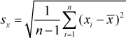, and the sample standard deviation of y is . A mathematically equivalent expression defines the sample correlation as the sum of the products of the standardized values , where and . The variable has a Student’s t-distribution (approximately) with n − 2 degrees of freedom and can be used to test if an r value is different from zero.

In Excel use CORREL(x_range, y_range), where x_range and y_range are ranges. CORREL will have an error if the variance of x or y is zero. The equivalent formula (n/(n−1))*COVAR(x_range, y_range)/ STDEV(x_range)/ STDEV(y_range) can also be used. The term n/(n−1) is needed because the Excel COVAR function is for the population rather than the sample.

The correlation between two sets of ranked values (x_i, y_i) can be found with the Spearman’s rank correlation coefficient, which is . However, if two or more ranks are tied for either set of numbers, the correlation coefficient (Pearson’s) should be used.

See autocorrelation, covariance, forecast error metrics, linear regression, variance.

cost center – An accounting term for an area of responsibility that is only held accountable for its cost.

Cost centers are often service and support organizations, such as manufacturing, human resources, and information technology, that do not have any easily assignable revenue.

See absorption costing, Activity Based Costing (ABC), human resources, investment center, profit center, revenue center.

cost driver – See Activity Based Costing (ABC).

cost of goods sold – An accounting term for all direct costs incurred in producing a product or service during a period of time; also called cost of goods, cost of sales, cost of products sold, and cost of production.

Cost of goods sold usually includes direct materials, incoming transportation, direct labor cost, production facilities, and other overhead (indirect) labor and expenses that are part of the manufacturing process. It does not include indirect costs, such as administration, marketing, and selling costs, that cannot be directly attributed to producing the product.

Inventory is an asset, which means it is not expensed when purchased or produced, but rather goes into an inventory asset account. When a unit is sold, the cost is moved from the inventory asset account to the cost of goods sold expense account. Cost of goods sold is on the income statement and used in the inventory turnover calculation.

See ABC classification, direct cost, direct labor cost, financial performance metrics, gross profit margin, inventory turnover, Last-In-First-Out (LIFO), overhead, transfer price.

cost of quality – A framework coined by quality leader Phillip Crosby and used to measure quality-related costs; now called the “price of non-conformance.”

The cost of quality concept was popularized by Phillip Crosby, a well-known author and consultant (Crosby 1979). Crosby focused on the following principles:

• Quality is defined as conformance to requirements.

• The system for causing quality is prevention, not appraisal.

• The performance standard is zero defects.

• The measurement of quality is the cost of quality (sometimes called the price of nonconformance).

More recently, Crosby has replaced “the cost of quality” with the “price of nonconformance” in response to quality professionals who did not like the older term. The price of nonconformance assigns an economic value to all waste caused by poor quality. Examples of the price of nonconformance include wasted materials, wasted capacity, wasted labor time, expediting, inventory, customer complaints, service recovery, downtime, reconciliation, and warranty.

According to Feigenbaum (1983), the cost of quality framework includes these four elements:

Prevention costs – Cost of designing quality into the product and process. This includes product design, process design, work selection, and worker training. Some authors also add the cost of assessing and improving process capability. Many firms find that this cost is hardest to measure.

Appraisal costs – Cost of inspection, testing, auditing, and design reviews for both products and procedures.

Internal failure costs – Cost of rework, scrap, wasted labor cost, wasted lost machine capacity, and poor morale. Lost capacity for a bottleneck process can also result in lost gross margin.

External failure costs – Costs incurred after the customer has taken possession of the product and include warranty, repair (both field repair and depot repair), lost gross margin/refunds, customer support, lost customer good will, damage to the brand, damage to channel partnerships, and lawsuits.

An important teaching point with this framework is that most organizations need to move the costs up the list. In other words, it is usually better to have internal failures than external failures. It is usually better to have appraisal than internal failure and usually better to have prevention than appraisal. A couple of metaphors are helpful here. It is better to avoid smoking (prevention) than to try to heal cancer. It is better to avoid toxic waste than to try to clean it up.

The “1-10-100 rule” suggests that $1 on prevention will save $10 in appraisal, $10 on appraisal will save $100 in internal failure, and $100 in internal failure will save $1000 in external failure. Of course, the numbers are not precise, but the concept is an important one.

The old saying “An ounce of prevention is worth a pound of cure” communicates the same concept. A similar old phrase “A stitch in time saves nine” suggests that timely preventive maintenance will save time later. In other words, sewing up a small hole in a piece of clothing will save time later.

See appraisal cost, early detection, inspection, prevention, process capability and performance, quality management, scrap.

Council of Logistics Management (CLM) – See Council of Supply Chain Management Professionals (CSCMP).

Council of Supply Chain Management Professionals (CSCMP) – A professional society with the mission “to lead the evolving Supply Chain Management profession by developing, advancing, and disseminating supply chain knowledge and research.”

Founded in 1963, the Council of Supply Chain Management Professionals (CSCMP) is an association for individuals involved in supply chain management. CSCMP provides educational, career development, and networking opportunities to its members. The National Council of Physical Distribution Management (NCPDM) was founded in 1963 by a group of educators, consultants, and managers who envisioned the integration of transportation, warehousing, and inventory as the future of the discipline. In 1985, the association changed its name to the Council of Logistics Management (CLM) and in 2005 changed its name to CSCMP.

CSCMP publishes a number of trade journals and the academic journal The Journal of Business Logistics. The CSCMP website is www.cscmp.org.

See operations management (OM).

counting tolerance – The margin for error used when counting items in an inventory.

An item count is considered wrong only when the count is off by more than the “counting tolerance,” which is usually a percentage defined for each category of items. High-value items will usually have a counting tolerance of zero; very low-value items might have a counting tolerance of 10% or more.

See cycle counting, tolerance.

covariance – A measure of the strength of association between two variables.

If two variables have high covariance, they tend to vary together. In other words, when one is higher (lower) than its mean, the other one is too. The mathematical definition of the sample covariance between random variables X and Y is , where and are the sample means. The first term is called the definitional form and the last term is called the computational form because it only requires a single pass for the summations. Covariance is related to correlation by the equation , which shows that correlation is the covariance “normalized” by the standard deviations of the two variables. Some basic facts about covariance for random variables X and Y and constants a and b: Cov(a, X) = 0, Cov(X, Y) = Cov(Y, X), Cov(X, X) = Var(X), Cov(aX, bY) = abCov(X, Y), Cov(X + a, Y + b) = Cov(X, Y).

The Excel population covariance is COVAR(x_range, y_range), where x_range and y_range are the x and y ranges. For the sample covariance, use (n/(n−1))COVAR. Note that this issue is not documented in Excel.

See Analysis of Variance (ANOVA), correlation, variance.

C_p – See process capability and performance.

CPFR – See Collaborative Planning Forecasting and Replenishment.

C_pk – See process capability and performance.

CPM – See Critical Path Method (CPM).

CRAFT – See facility layout.

crashing – See critical path.

critical chain – The set of tasks that determines the overall duration of a project, taking into account both precedence and resource dependencies.

The critical chain is similar to the critical path except that it goes one major step further and factors in resource constraints. The steps in the critical chain approach are as follows:

Step 1. Compute the early start, early finish, late start, late finish, and slack times as is normally done with the critical path method – The path through the network with the longest total time is called the critical path, which is the path (or paths) with the shortest slack. The estimated task times for this process should be set at the median rather than the 90-99% point of the task time distribution.

Step 2. Create a detailed schedule, starting from the current date and moving forward in time – When a task is complete, begin the next task in the precedence network if the required resources are available. When a resource becomes available, assign it to the task that has the least amount of slack time as computed in Step 1. Continue this process until the schedule is complete for all activities. This new schedule is called the critical chain and will be longer than the critical path, which only considers the precedence constraints. The critical chain will still follow the precedence constraints, but will never have any resource used more than its capacity.

Step 3. Strategically add time buffers to protect activities on the critical chain from starting late – Noncritical chain activities that precede the critical chain should be planned to be completed early so the critical chain is protected from disruption.

The consulting/software firm Realization markets software called Concerto that implements critical chain concepts in Microsoft Project.

See critical path, Critical Path Method (CPM), Earned Value Management (EVM), Project Evaluation and Review Technique (PERT), project management, safety leadtime, slack time, Theory of Constraints (TOC).

critical incidents method – An approach for identifying the underlying dimensions of customer satisfaction.

The critical incidents method involves collecting a large number of customer (or worker) complaints and compliments and then analyzing them to identify the underlying quality dimension (timeliness, friendliness, etc.). It is important to note that in analyzing a complaint or a complement, it does not matter if it is a negative (complaint) or a positive (compliment); the goal is to simply identify the underlying dimensions of quality, regardless if they are satisfiers or dissatisfiers.

This technique is useful for identifying the key dimensions of service quality for a customer satisfaction survey. This technique can also be used in other contexts, such as job analysis to identify the critical dimensions of worker satisfaction.

See service quality, voice of the customer (VOC).

critical path – The longest path through a project-planning network; the path that has the least slack (float) time.

The only way to reduce the project completion time is to reduce the task times along the critical path. Task times on the critical path are usually reduced by applying more resources (people, money, equipment, etc.) or by overlapping activities that were originally planned to be done sequentially. Reducing times along the critical path is called crashing, schedule compression, and fast tracking. Crashing non-critical activities will not improve the project completion time. Crashing should focus on the critical path tasks that have the lowest cost per unit time saved.

The Critical Path Method entry explains the methodology for finding the critical path. Activities not on the critical path can become critical if they are delayed. Therefore, project managers need to monitor schedules and practice risk management. It is possible for a network to have two or more critical paths.

A critical chain is similar to a critical path, but the two concepts are not synonymous. The critical chain considers resource constraints, whereas the critical path does not.

See critical chain, Critical Path Method (CPM), Failure Mode and Effects Analysis (FMEA), project management, slack time.

Critical Path Method (CPM) – An approach for project planning and scheduling that focuses on the longest path through the project planning network.

Project scheduling begins with the work breakdown structure that defines the “tree” of activities that make up the project. Each task at the bottom of the tree is then defined in terms of a task name, task time, resources (people, machines, money, etc.), and a set of precedence relationships, which is the set of tasks that need to be completed before the task can be started.

Simple CPM project network example

The simple example to the right shows the scheduling process with a project network with five tasks (A-E) with the times (in days) noted by each task. The process has two passes: a forward pass to create the early start and early finish times, and a backward pass to create the last finish and late start times for each task.

The forward pass begins with task A, which has an early start at the beginning of day 1 (ES = 1) and an early finish at the end of day 1 (EF = 1). Task B cannot start until task A is completed and therefore has an early start at the beginning of day 2 (ES = 2). Task B requires 2 days and has an early finish at the end of day 3 (EF = 3). The forward pass continues until every node is assigned an early start (ES) and early finish (EF).

The backward pass (back scheduling) begins with the desired completion date for the project, which is the late finish for the last task (task E). The required completion date for this project is the end of day 11 (i.e., LF = 11). Planning backward from this completion date, task E has a late start date at the beginning of day 10 (LS = 10). Continuing this backward pass creates the late finish and late start for all nodes. The notation in parentheses beside each task node is (Early Start, Late Start, Early Finish, Late Finish) = (ES, LS, EF, LF).

The slack time (float) for any task is the difference between the early start and the late start (i.e., LS – ES), which is always the same as the difference between the early finish and late finish (i.e., LF – EF). The critical path is the path through the network that has the smallest slack. In this example, the critical path is A→D→E. The slack time for a task may be zero or negative.

Management should prioritize tasks along the critical path for both resource allocation and crashing. When a resource (e.g., person, tool, or machine) becomes free, a good rule for re-allocating this resource is to use the minimum slack rule, which simply assigns the resource to the open task that has the least slack. This is essentially the same process used to identify the critical chain.

If it is necessary to reduce the total project time, the project manager should find the task on the critical path that can be reduced (crashed) at the lowest cost per unit time, make the change, and then repeat the crashing process until the desired project completion time is achieved or until the cost exceeds the benefit. Crashing noncritical activities will not improve the project completion date.

Activities not on the critical path can become critical if they are delayed. This suggests that project managers need to constantly monitor project schedules and practice good risk management to prepare for contingencies. Note that it is possible for a project network to have two or more critical paths.

The above figure uses the “activity-on-node” approach. The alternative “activity-on-arc” approach is presented in some textbooks, but is far more difficult to understand and is rarely used in practice.

Two of the better-known project scheduling packages are Microsoft Project and Primavera sold by Oracle. Microsoft Project is said to be better for smaller projects and Primavera better for larger projects. Many other commercial packages are available.

See back scheduling, critical chain, critical path, forward scheduling, Gantt Chart, load leveling, Project Evaluation and Review Technique (PERT), project management, project network, slack time, work breakdown structure (WBS).

critical ratio – See dispatching rule, newsvendor model.

Critical to Quality (CTQ) – Key measurable characteristics of a product or process that require performance standards or specification limits to satisfy the customer (internal or external) requirements; also called Key Process Output Variable (KPOV).

CTQ may include the upper and lower specification limits or any other factors related to the product or service. A CTQ usually must be interpreted from a qualitative customer statement to an actionable, quantitative business specification. CTQs are what the customer expects of a product. The customer’s requirements must be expressed in measurable terms using tools, such as DFMEA.

See Key Process Output Variable (KPOV), lean sigma, quality management, voice of the customer (VOC).

CRM – See Customer Relationship Management (CRM).

cross-functional team – A group of employees from different parts of an organization who come together and use their different viewpoints and skills to address a problem.

Many organizational problems cannot be solved by a single business function. For example, a new product development project might require expertise from marketing, sales, manufacturing, and engineering. Crossfunctional teams are often the best approach for addressing these problems. A cross-functional team may be self-directed or directed by a sponsor (or sponsors) within the organization. Cross-functional teams are a common component of concurrent engineering, agile software development, and lean sigma projects.

See agile software development, concurrent engineering, lean sigma, organizational design, project management, Quality Function Deployment (QFD), red tag, sponsor.

cross-docking – A warehousing term for the practice of moving products directly from incoming trucks or rail cars to outgoing trucks without placing inventory on shelves in the warehouse or distribution center; also called crossdocking and cross docking.

Products that are good candidates for cross-docking have high demand, standardized packaging, and no special handling needs (e.g., security or refrigeration). This is a common strategy for retail distribution where trucks carry large shipments from factories to the cross-dock facility, which loads other trucks with mixed assortments to send to retail stores.

Cross-docking has many advantages over traditional warehouse facilities:

• Reduced inventory and carrying cost – The firm replaces inventory with information and coordination.

• Reduced transportation cost – For less than truck load (LTL) and small package carriers, cross-docking is a way to reduce transportation costs by consolidating shipments to achieve truck load quantities.

• Reduced labor cost – Cross-docking avoids costly moves to and from shelves in the warehouse.

• Improved customer service – Cross-docked shipments typically spend less than 24 hours in a cross-dock.

The figure on the right shows a cross-docking process with a top-down view of eight trucks. Four trucks bring products in from suppliers and four take products out to the retail stores.

Napolitano (2000) proposed the following classification scheme for cross-docking:

Manufacturing cross-docking for receiving and consolidating inbound supplies to support Just-in-Time manufacturing. For example, a manufacturer might lease a warehouse close to its plant and use it to prep subassemblies or consolidate kits of parts. Because demand for the parts is known, say from the output of an MRP system, there is no need to maintain stock.

Distributor cross-docking for consolidating inbound products from different vendors into a multi-SKU pallet, which is delivered as soon as the last product is received. For example, computer distributors often source components from different manufacturers and consolidate them into one shipment in merge-in-transit centers before delivering them to the customer.

Transportation cross-docking for consolidating shipments from different shippers in the LTL and small package industries to gain economies of scale. For small package carriers, material movement in the cross-dock is by a network of conveyors and sorters; for LTL carriers it is mostly by manual handling and forklifts.

Retail cross-docking for receiving product from multiple vendors and sorting onto outbound trucks for different stores. Cross-docking is one reason Walmart surpassed Kmart in retail sales in the 1980s.

Opportunistic cross-docking is transferring an item directly from the receiving dock to the shipping dock to meet a known demand in any type of warehouse.

All of the cross-docking practices involve consolidation and short cycle times, usually less than a day. Short cycle time is possible because the destination for an item is known before or upon receipt.

See Advanced Shipping Notification (ASN), consolidation, distribution center (DC), distributor, dock, economy of scale, forklift truck, less than truck load (LTL), logistics, Over/Short/Damaged Report, receiving, supply chain management, Transportation Management System (TMS), warehouse, Warehouse Management System (WMS).

cross-selling – A sales and marketing term for the practice of suggesting related products to a customer during a sales transaction or a customer service encounter.

In contrast to cross-selling, up-selling is a sales technique where a salesperson attempts to persuade the customer to purchase better or more expensive items. Cross-selling and up-selling can sometimes be combined to increase the value added for the customer and also increase the sales and margin for the selling organization.

See call center, Customer Relationship Management (CRM), customer service, order entry.

cross-training – Training workers in several different areas or functions outside their normal job responsibilities.

Having workers learn a wide variety of tasks has many advantages:

Increased flexibility – Workers can provide backup when the primary worker is unavailable or when the demand exceeds the capacity. This makes it easy to improve flow and reduce inventory. This increased flexibility allows the line workers to dynamically balance the line without any help from an industrial engineer.

Process improvement – When workers have a broader understanding of the organization, they can be more knowledgeable about how to improve it.

Develops human capital – Cross-trained workers are more valuable to the company and often find more satisfaction in their jobs. Cross-training is often an investment in the future for a firm.

See cellular manufacturing, facility layout, human resources, job design, job enlargement, job rotation, lean thinking, learning organization, line balancing, on-the-job training (OJT), workforce agility.

Croston’s Method – A time series forecasting method that is used for lumpy (intermittent) demand.

When the demand (sales) history for an item has many periods with zero demand, it is said to have intermittent or lumpy demand. Exponential smoothing does a poor job of forecasting lumpy demand because the exponentially smoothed average will approach zero after several zero demand periods and the forecast for the period with the next “demand lump” will therefore be close to zero. Exponential smoothing, therefore, should not be used for lumpy demand. A demand time series is often judged to be lumpy when the coefficient of variation of the demand is greater than one.

Croston (1972) suggests a method for forecasting lumpy demand by decomposing the time series into (1) the average size of the demand lumps and (2) the average time between the demand lumps. Croston’s Method uses simple exponential smoothing (SES) for the average size of the demand lumps and also for the average number of periods between the demand lumps. As shown in the table below, it implements three recursive equations.

Croston’s Method rules

The first equation updates the smoothed average size of the non-zero demand z_t. If the demand in period t is zero (i.e., d_t = 0), the average size of the demand remains unchanged; otherwise, the average size of a non-zero demand (z_t) is updated with simple exponential smoothing. The second equation updates the average number of periods since the last non-zero demand (p_t) based on q_t, which is the number of periods since the last demand. When the demand is zero, p_t remains unchanged; otherwise, p_t is updated with simple exponential smoothing based on q_t. The third equation updates q_t, which counts the number of periods between non-zero demand. If d_t is zero, the number of periods since the last demand is incremented by 1; otherwise, the number of periods since the last demand is reset to 1.

The forecast for the demand in period t + n is then f_t+n = z_t/P_t. If every period has a non-zero demand (i.e., p_t = 1), Croston’s Method is equivalent to simple exponential smoothing with smoothing constant α.

The SAP Library (http://help.sap.com/saphelp_scm50/helpdata/en/ac/216b89337b11d398290000e8a49608/content.htm) recommends initializing {z₀, p₀} = {0, 2} if d₁ = 0 and {d₁, 1} if d₁ > 0. However, this will create forecasts f_t = 1 for all periods when no non-zero demand is encountered. Therefore, the values z₀ = 0 if d₁ = 0 and z₀ = d₁ if d₁ > 0 are more logical. The q₀ parameter should be initialized at 1.

An alternative approach is to increase the size of the time buckets so that zero demands are rare or use the average demand over several periods. It is important to avoid using exponential smoothing for intermittent demand because it will forecast relatively high demand right after a “lump” in demand and forecast nearly zero demand about the time the next “lump” in demand occurs.

See coefficient of variation, exponential smoothing, forecasting, lumpy demand, time bucket, time series forecasting.

CRP (Capacity Requirements Planning) – See Capacity Requirements Planning (CRP).

CTO – See configure to order (CTO).

CTQ – See Critical to Quality (CTQ).

cube utilization – A warehousing term for the percent of the usable three-dimensional space (volume) used in a trailer, container, or warehouse.

Volume is calculated as the product of the three dimensions – width x height x depth.

See operations performance metrics, shipping container, slotting, trailer, warehouse.

cumsum chart – See cumulative sum control chart.

Cumulative Distribution Function (CDF) – See probability density function.

cumulative leadtime – The critical path leadtime (longest) required to purchase material and create a product to offer to the market; also known as the stacked leadtime.

The cumulative leadtime usually is the time required to purchase materials, fabricate (cut, mold, weld, finish, etc.), assemble, test, package, and ship a product assuming that no inventory is on hand and no materials have been ordered. The customer leadtime might be much less than the cumulative leadtime if intermediate products (e.g., subassemblies) are inventoried.

See customer leadtime, leadtime, planning horizon, push-pull boundary, time fence.

cumulative sum control chart – A quality and industrial engineering term for a graphical tool (chart) that plots the cumulative sum of deviations over time; also known as a cumsum control chart or cumsum chart.

A cumulative sum control chart plots the cumulative sum of deviations of successive samples from a target value , where S_m is the cumulative sum, x_i is the observed value (or sample mean), and μ is the target value. This can also be defined recursively as S_m = S_{m − 1} + x_i − μ. This concept is very similar to a tracking signal used for forecasting.

See control chart, Statistical Process Control (SPC), Statistical Quality Control (SQC), tracking signal.

current reality tree – A Theory of Constraints term for a causal map that describes the current state of a problem.

See causal map, future reality tree, Theory of Constraints (TOC).

Customer Effort Score (CES) – A measure of service quality using the single question “How much effort did you personally have to put forth to handle your request?”

Dixon, Freeman, and Toman (2010) developed this simple scale for call centers, service centers, and self-service operations. They argue that customers do not want to be delighted; they just want their needs met without annoying phone calls, transfers, and confusion. They claim that the CES is more predictive of customer loyalty than the Net Promoter Score (NPS) and direct measures of customer satisfaction. They recommend using a CES scale from 1 (very low effort) to 5 (very high effort) and suggest that service providers intervene when customers report a high CES. Note that CES is a measure of dissatisfaction and NPS is a measure of satisfaction.

See Net Promoter Score (NPS), operations performance metrics, service management, service quality.

customer leadtime – The planned or actual time in system for a customer (or customer order); planned or actual turnaround time.

Customer leadtime is the difference between the time the customer (or order) enters the system and the time that the customer (or order) is complete. The term “leadtime” suggests that this term should refer to a planning factor rather than the actual time or the historical average leadtime.

In a manufacturing context, the customer leadtime begins after the push-pull boundary, which is the location in the process where the firm no longer stocks inventory. Customer leadtime can be nearly zero if the manufacturer has the push-pull boundary at finished goods inventory. In a retail context, customer leadtime is the difference between the time the customer selected and received an item.

See addition principle, assemble to order (ATO), cumulative leadtime, leadtime, postponement, push-pull boundary, respond to order (RTO), time in system, turnaround time.

customer profitability – The revenue a customer generates minus the costs needed to acquire and retain that customer.

Customer profitability is closely related to the concepts of customer equity and lifetime value. Without a method for estimating customer profitability, a firm may spend scarce marketing dollars to retain its unprofitable (or low profit) customers and may mistreat its most profitable customers.

See Activity Based Costing (ABC), Customer Relationship Management (CRM).

Customer Relationship Management (CRM) – An information system that collects data from a number of customer-facing activities to help an organization better understand its customers so that it can better match its products and services to customer needs and thereby increase sales.

Although CRM involves information technology, it is fundamentally a strategic process (and not just an IT project) for helping organizations better understand their customers’ needs, better meet those needs, and increase sales and profits. CRM processes and systems combine information from marketing, sales, contact management, and customer service activities. CRM also provides tools to analyze customer/product sales history and profitability, campaign tracking and management, contact and call center management, order status information, and returns and service tracking. A good CRM system provides many benefits:

• Provide exactly the services and products that customers want.

• Offer better customer service.

• Allow for more effective cross-seling (selling complementary products).

• Help sales staff close deals faster.

• Help the firm retain current customers and discover new ones.

• Collect timely complete information on customers through multiple customer interfaces, including call centers, e-mail, point-of-sale operations, and direct contact with the sales force.

• Reduce the transaction cost for buying products and services.

• Provide immediate access to order status.

• Provide support that will reduce the costs of using products and services.

• Help management develop a deeper understanding of customer buying behavior “sliced and diced” in a number of ways, such as geography, demographics, channel, etc.

See cross-selling, customer profitability, customer service, target price, voice of the customer (VOC).

customer satisfaction – See service quality.

customer service – (1) The organization charged with dealing with customer complaints and other customer needs. (2) A metric used to evaluate how well an organization or an inventory is meeting customer requirements.

See Automatic Call Distributor (ACD), call center, cross-selling, Customer Relationship Management (CRM), empowerment, fulfillment, order entry, service level, service quality, SERVQUAL, supplier scorecard, Third Party Logistics (3PL) provider.

customization flexibility – See flexibility.

customization point – See push-pull boundary.

cycle counting – A methodology for counting items in storage that counts more important items more often and systematically improves the record-keeping process.

Instead of counting all items with a year-end physical inventory count, cycle counting counts items throughout the year, with the “important” items counted much more often than other items. Cycle counting is an application of Pareto’s Law, where the “important few” items are counted often and the “trivial many” items are counted infrequently.

The benefits of a good cycle counting program over a physical inventory are summarized in the table below. The main benefits of cycle counting are (1) it is better at finding and fixing the problems that cause inaccurate inventory balances and (2) it maintains record accuracy throughout the year.

Year-end inventory versus cycle counting

Source: Professor Arthur V. Hill

Some factors to consider when determining how often to count an item include:

• Criteria set by accounting and external auditors for the elimination of the annual physical inventory count.

• External regulations that require specific count frequencies.

• Annual dollar volume of an item (also known as the annual cost of goods sold).

• Annual unit volume of an item (number of units sold).

• Unit cost of an item.

• Pilferage risk associated with the item.

• Current inventory accuracy level for that particular item.

Some rules for determining how often to count an item include (1) count items with higher annual dollar volume more often (the ABC system), (2) count just before an order is placed, (3) count just before a new order is placed on the shelf, (4) count when the physical inventory balance is zero, (5) count when the physical inventory balance is negative, and (6) count after a specified number of transactions. Rules 2 and 3 are ways to implement rule 1 because “A” items will be ordered more often. Rule 3 minimizes the number of units that need to be counted because the shelf is nearly empty when an order arrives. Rules 2 and 3 can be implemented so that every n-th order is counted. Rule 5 is a good rule to use along with any other rule.

An item count is considered wrong only when the count is off by more than the counting tolerance, which is usually a percentage defined for each category of items. High-value items will usually have a counting tolerance of zero; low-value items might have a counting tolerance of 10% or more.

With a blind count the counter is given the item number and location but no information about the count currently in the database. This approach avoids giving counters reference points that might bias their counts.

Tompkins Associates provides more information on this topic at tompkinsinc.com/publications/monograph/monographList/WP-19_Cycle_Counting.pdf?monographID=WP-19.

See ABC classification, backflushing, learning organization, on-hand inventory, Pareto’s Law, physical inventory, scale count, shrinkage.

cycle service level – See safety stock.

cycle stock – The inventory due to lotsize quantities greater than one; also called the lotsize inventory.

Cycle stock follows a “saw tooth” pattern (see the reorder point entry for an example). For instantaneous replenishment and constant average demand, the average cycle stock is Q/2, where Q is the fixed order quantity. Organizations can reduce cycle stock by reducing lotsizes and lotsizes can be reduced economically by reducing the order (setup) cost. The setup time reduction methods entry provides a methodology for reducing setup cost.

See commonality, Economic Order Quantity (EOQ), instantaneous replenishment, lotsize, safety stock, setup time reduction methods.

cycle time – (1) The time between completions (or starts) of a unit of work. (2) The time from beginning to end for a unit of work (also known as throughput time, flow time, and turnaround time).

These two definitions are quite different, but both are used in practice.

Definition 1: For decades, industrial engineers defined cycle time as the time between completions (or starts) of a process step. For example, this could be measured as the time between units “falling off” the end of a manufacturing process or the maximum work time allowed for each worker on an assembly line. In lean terminology, the target cycle time (time between completions) aligned to the market demand rate is called the takt time (see the entry for takt time). This is the definition for cycle time used in LEI’s Lean Lexicon (Marchwinski & Shook 2006).

Definition 2: Cycle time can also be defined as the cumulative time (also called total throughput time, total flow time, and production leadtime) required for a unit from start to end and can be measured as the completion time minus the start time for the same unit.

The first definition is the time between completions and the second definition is the time to complete one unit. The second definition (throughput time) has become the more widely used term in practice in North America, and it is now common to use the terms throughput time (or flow time) and cycle time synonymously.

To compare the two definitions of cycle time, imagine an assembly line in an appliance factory that has one dishwasher coming off the end of the line every two minutes. Each of the 20 steps in the assembly process requires exactly two minutes. Using the first definition, this is a cycle time (time between completions) of two minutes. However, using the second definition, a dishwasher that started at 8:00 am will not be complete until 8:40 am (20 steps times two minutes each), which means that the assembly line has a cycle time (throughput or flow time) of 40 minutes. The first definition focuses on the time between units being completed for each step in the process, whereas definition two focuses on the time to complete one unit from beginning to end for the entire process.

Although it is fairly easy to measure the average cycle time (throughput time) for a manufacturing order in a factory, it is often difficult to estimate the average cycle time (throughput time) for a complex product because it is not clear when the product is started. Given that each required component might have a different starting time, it is hard to determine the total cycle time for the completed product. A simple approach for estimating the cycle time (and also the periods supply) is to use the inverse of the inventory turnover ratio for the work-in-process (WIP) inventory. Therefore, if the WIP inventory turnover for a product is four turns per year, the “dollar weighted cycle time” is three months.

In queuing theory terms, the average completion rate will be the same as the average production rate (assuming that no units are lost and that sufficient capacity is available). With a production rate λ (lambda), the average time between starts and average time between completions is 1/λ. According to Little’s Law (Little 1961), the average work-in-process inventory is L_s = λW_s, where W_s is the average time in the system. Building on the previous example, the average time between completions was two minutes, which means that the production rate is λ = 1/2 units/minute. Given that the throughput time was W_s = 40 minutes, the average number of units in process is units. See the queuing theory and Little’s Law entries for more details on these issues.

Many practitioners use the terms “cycle time” (as in throughput time) and “leadtime” synonymously. However, in this author’s opinion, it is better to use the term “leadtime” as a planning factor (as in planned leadtime) rather than as the actual throughput time for an order. The leadtime entry discusses these issues.

See assembly line, balanced scorecard, inventory turnover, leadtime, Little’s Law, operations performance metrics, order-to-cash, periods supply, pitch, purchasing leadtime, station time, takt time, time in system, touch time, turnaround time, value added ratio, wait time.

cycle time efficiency – See value added ratio.