J

JCAHO – See Joint Commission.

jidoka – The Toyota Production System practice of designing processes and empowering workers to shut down a process when an abnormal condition occurs; sometimes called autonomation.

The Japanese word “jidoka” is often translated as “autonomation,” which is a contraction of the words “autonomous” and “automation.” Jidoka is sometimes translated as “automation with a human touch (or human mind).” According to Ohno (1978), the original jidoka device was a loom developed by Sakichi Toyoda (1867-1930), the founder of the Toyota Motor Company. This loom stopped instantly if any one of the threads broke so defective products were not built and so problems could be seen immediately. According to Ohno (1979), Toyota sold the patent for his loom in 1930 to the Platt Brothers in England for $500,000, and then invested this money in automobile research, which later led to the creation of the Toyota Motor Company.

Originally, jidoka focused on automatic methods for stopping a process when an error condition occurred; however, it is now used to describe both automated and human means for stopping a process when a problem occurs. For example, a process can use limit switches or devices that will automatically shut down the process when the required number of pieces has been made, a part is defective, or the mechanism jams. This same process can be operated with policies that allow the operators to shut down the machine when a warning light goes on.

Quality benefits of jidoka – Jidoka causes work to stop immediately when a problem occurs so defective parts are never created. In other words, Jidoka conducts 100 percent inspection, highlights the causes of problems, forces constant process improvement, and results in improved quality. Whereas automation focuses on labor reduction, jidoka (autonomation) focuses on quality improvement. Note that jidoka is closely related to Shigeo Shingo’s concept of poka yoke.

Cost benefits of jidoka – Jidoka frees equipment from the necessity of constant human attention, makes it possible to separate people from machines, allows workers to handle multiple operations, and prevents equipment breakdowns. Ideally, jidoka stops the line or machine automatically, which reduces the burden of workers to monitor the process. In fact, many sources define jidoka as stopping production automatically when a problem occurs.

Jidoka is often implemented with a signal to communicate the status of a machine. For example, a production process might use andon lights with a green light if everything is okay, a yellow light to signal an abnormal condition, and a red light if the process is stopped.

See andon light, automation, autonomation, empowerment, error proofing, lean thinking, multiple-machine handling, Toyota Production System (TPS).

jig – A mechanical device that holds a work piece securely in the correct position or has the capability of guiding the tool during a manufacturing operation.

See fixture, manufacturing processes, tooling.

JIT – See Just-in-Time (JIT).

JIT II – A practice of having supplier representatives work at a customer location to better facilitate product design or production coordination activities.

The JIT II concept was developed by Lance Dixon at Bose Corporation (Porter & Dixon 1994). JIT II is essentially vendor managed inventory (VMI), early supplier involvement, and co-location of personnel. The term does not appear to be widely used.

See co-location, Early Supplier Involvement (ESI), lean thinking, vendor managed inventory (VMI).

job – (1) In a general context: Any work that needs to be done by an individual or a machine. (2) In a manufacturing context: Work that is done to create a batch of an item in response to a customer request; also known as an order, manufacturing order, or production order.

See job order costing, job shop, lotsize.

job design – The process of defining and combining tasks to create work for an individual or a group of individuals; also called work design and socio-technical design.

Job design usually results in a job description, which defines the set of tasks and responsibilities for an individual worker. Job design should consider organizational requirements, individual worker attributes, health, safety, and ergonomics. Taylor’s scientific method tended to view job design as a pure engineering problem; however, the human relations movement broadened the scope to consider job satisfaction, motivation, and interpersonal issues.

Organizations can better achieve their objectives by designing work that motivates workers to achieve their full potential. A deep understanding of job design requires an understanding of behavioral science, organizational behavior, organizational design, psychology, human resources management, economics, operations, and engineering.

Socio-technical design considers the interaction between people and the technological processes in which they work. Socio-technical design is important in almost every operations management topic. For example, visual control, a key lean manufacturing concept, is a good socio-technical design because when processes are made more visual, workers can understand them better and be more productive.

See addition principle, cellular manufacturing, cross-training, division of labor, empowerment, ergonomics, gainsharing, Hawthorne Effect, High Performance Work Systems (HPWS), human resources, job enlargement, job rotation, labor grade, lean thinking, multiplication principle, New Product Development (NPD), on-the-job training (OJT), organizational design, pay for skill, productivity, RACI Matrix, Results-Only Work Environment (ROWE), scientific management, self-directed work team, Service Profit Chain, single point of contact, standardized work, subtraction principle, work measurement, work simplification, workforce agility.

job enlargement – Adding more tasks to a job; increasing the range of the job duties and responsibilities.

The management literature does not have consistent definitions of the terms “job enlargement” and “job enrichment.” However, most experts define the terms as follows:

Job enlargement – This is also called horizontal job enlargement and adds similar tasks to the job description. In other words, the worker is assigned more of a co-worker’s job. For example, the worker who cleans sinks also is assigned to clean the toilets.

Job enrichment – This is sometimes called vertical job enlargement and adds more decision rights and authority to the job. In other words, the worker is assigned some of the boss’ job. For example, the worker might be given the added responsibilities of scheduling and inspecting the bathroom cleaning process for other workers.

Job enlargement can have many benefits for an organization. Some of these include:

Reduced cycle time – When workers have broader skills, they can be moved to where they are needed. This reduces queue time and cycle time.

Fewer queues – When a worker is assigned to do two steps instead of one, the queue between the steps is eliminated, and much of the associated wait time is eliminated.

Improved process improvement capability –Workers with broader experience are better able to help the organization improve processes, which means that the organization can accelerate “learning.”

Improved worker morale and retention – Enlarged jobs are often more interesting, which improves worker morale and retention.

See addition principle, Business Process Re-engineering (BPR), cross-training, division of labor, empowerment, handoff, human resources, job design, job rotation, learning organization, organizational design, pay for skill, standardized work, work simplification.

job enrichment – See job enlargement.

job order costing – A cost accounting approach that accumulates costs for a job as it passes through the system; also known as job costing.

A job order costing system will accumulate the standard (or actual) direct labor, direct materials, and overhead costs as a job passes through each step in a process. This type of system makes the most sense for a process layout, such as a job shop.

See backflushing, facility layout, job, job shop, overhead, target cost.

job rotation – The movement of workers between different jobs in an organization.

This policy can be an effective method for cross-training and can improve communications, increase process understanding, and reduce stress and boredom. Job rotation can also prevent muscle fatigue and reduce workplace injuries.

Job rotation also makes sense for managers. The vice president of Emerson/Rosemount in Eden Prairie, Minnesota, had been the vice president of Engineering, vice president of Manufacturing, and vice president of Marketing before being named the president of the division. This executive was well prepared for a general management role because of his job rotation experiences.

See cross-training, human resources, job design, job enlargement, learning organization, pay for skill, workforce agility.

job shop – A manufacturing facility (or department in a facility) that groups similar machines in an area and makes customized products for customers.

A job shop makes customized products with a make to order (MTO) customer interface in a process layout. This customization is accomplished by moving customer orders through one or more departments (workcenters) to complete all of the steps (operations) on the routing. Job shops typically have long customer leadtimes, long queues, highly skilled workers, and general purpose machines. One of the main challenges for a job shop is promising completion dates to customers and then scheduling orders to reliably deliver the jobs on or before the promised date.

For example, a machining job shop might have drills, lathes, and grinding machines in separate workcenters. Almost every order going through the job shop is unique in terms of the engineering specifications, routings, and order sizes. The job shop has a long queue of orders waiting at each machine in order to maintain reasonably high utilization of the equipment and skilled machine operators.

In contrast, a product layout organizes people and equipment in the sequence required to make the product. For example, an assembly process is often organized in a straight line in the sequence required to build the product. Assemblies are moved one at a time from one assembly step to the next. Some workers may require tools and machines for their step in the process. All products go through exactly the same sequence, very little product variety is allowed, no queues are allowed between steps, and parts are moved very short distances by hand in lotsizes of one unit.

See batch process, discrete manufacturing, dispatching rules, facility layout, flowshop, job, job order costing, job shop scheduling, makespan.

job shop scheduling – The process of creating a schedule (or sequence) for jobs (orders) that will be processed in a job shop.

Job shops must make order date promises to customers when the jobs arrive. However, the uncertainty in queue times, setup times, and run times makes it difficult to predict when an order will be completed. One of the main performance metrics used in most job shops is the percentage of orders that are on time with respect to the original promise date. Although many managers agree that it would be better to measure against the original customer request date, few firms use this policy. Some firms follow the poor management practice of allowing the promise date to be changed after the promise was made to the customer, and then measure their performance against the revised promised date.

Academic research in job shop scheduling divides problems into two classes: static and dynamic. In the static problem, the set of jobs is given and does not change. The static problem is usually defined as minimizing the average flow time or the makespan (the ending time for the last job). Historically, the academic research in job shop scheduling has focused on simulation experiments that compare dispatching rules and developing both exact and heuristic finite scheduling algorithms that create schedules that do not violate the capacity constraints. Exact methods often require inordinate amounts of computing time, but guarantee the optimal (mathematically best) solution; heuristic methods are computationally fast, but do not guarantee the optimal solution. See the dispatching rules entry for more detail.

Most Advanced Planning and Scheduling (APS) systems, such as I2, Manugistics, and SAP APO, have scheduling capabilities for job shop scheduling. However, in this author’s experience, these systems are often difficult to understand, implement, and maintain because of the data requirements, complexity of the problems, and complexity of the systems.

See Advanced Planning and Scheduling (APS), algorithm, dispatching rules, expediting, flowshop, heijunka, job shop, makespan, service level, shop floor control, slack time.

jobber – See wholesaler.

Joint Commission – An independent, not-for-profit organization that sets healthcare quality standards and accredits healthcare organizations in the United States; formerly called the Joint Commission on Accreditation of Healthcare Organizations (JCAHO), but now officially called The Joint Commission” and abbreviated TJC.

The Joint Commission is an independent, not-for-profit organization in the U.S. that is governed by a board of physicians, nurses, and consumers. It evaluates and accredits more than 15,000 healthcare organizations and programs in the U.S. Its mission is “To continuously improve the safety and quality of care provided to the public through the provision of healthcare accreditation and related services that support performance improvement in health care organizations.” Its “positioning statement” is “Helping Health Care Organizations Help Patients.” The Joint Commission’s standards address an organization’s performance in key functional areas. Each standard is presented as a series of “Elements of Performance,” which are expectations that establish the broad framework that its surveyors use to evaluate a facility’s performance.

The Joint Commission’s homepage is www.jointcommission.org.

See adverse event, sentinel event.

joint replenishment – The practice of ordering a number of different products on a purchase or manufacturing order to reduce the ordering (setup) cost.

In the purchasing context, inventory management cost can often be reduced by ordering many items from a supplier on the same purchase order so the transaction and shipping costs are shared by many items. One simple joint replenishment policy is to trigger a purchase order for all items purchased from a supplier when one item reaches a reorder point. Order quantities can be determined using an order-up-to level policy subject to minimum order quantities and package size multiples. In a manufacturing context, joint replenishment is important when a process has major setups between families of products and minor setups between products within a family. When one product needs to be made, the firm makes many (or all) products in the family.

See inventory management, lotsizing methods, major setup cost, order-up-to level, purchasing, setup cost.

joint venture – A legal entity formed between two or more parties to undertake an activity together; commonly abbreviated as JV.

JVs normally share profits, risk, information, and expertise. JVs are common in oil exploration and international market entry. Many JVs are disbanded once the activity is complete.

See Third Party Logistics (3PL) provider, vertical integration.

just do it – A very small process improvement task or project; also called quick hits.

Most process improvement projects are able to identify a number of small “just do it” improvement tasks. These just do it tasks can be done by one person, require less than a day, do not normally require sign-offs by quality control or higher-level managers, and do not require significant coordination with other people. The “just do it” slogan is a trademark of Nike, Inc., and was popularized by Nike shoe commercials in the late 1980s.

Examples of just do it tasks include calling a supplier to request that they avoid deliveries over the noon hour, improving safety by attaching a power wire to a wall, or adding a sign to a storage area.

Process improvement teams should quickly implement these small improvements and not waste time prioritizing or discussing them. However, it is important that project teams document the benefits of these tasks so leaders can learn about the improvement opportunities and implement similar ideas in other areas, and include the benefits of the just do it tasks when evaluating the contributions of the project team.

See lean sigma, project management, quick hit.

Just-in-Time (JIT) – A philosophy developed by Toyota in Japan that emphasizes manufacturing and delivery of small lotsizes only when needed by the customer.

JIT primarily emphasizes the production control aspects of lean manufacturing and the Toyota Production System (TPS). For all practical purposes, the term “JIT manufacturing” has disappeared from common usage in North America. The concept of “lean manufacturing” is now considered more current and larger in scope.

See kanban, lean thinking, Toyota Production System (TPS).

K

kaikaku – A Japanese word meaning radical change, breakthrough improvement, transformation, or revolution.

Kaikaku is a major, significant improvement that occurs after many small, incremental improvements (kaizen events). Kaikaku should come naturally after completing many kaizens. The kaizens make kaikaku possible because they simplify the process and make it more visible. Kaizen is essential for a long-term lean transformation, but kaikaku is sometimes necessary to achieve breakthrough performance.

See Business Process Re-engineering (BPR), kaizen, kaizen workshop.

kaizen – A Japanese word meaning gradual and orderly continuous improvement or “change for the better.”

The English translation is usually continuous (or continual) improvement. According to the kaizen philosophy, everyone in an organization should work together to make improvements. It is a culture of sustained continuous improvement focusing on eliminating waste in all systems and processes of an organization. Kaizen is often implemented through kaizen events (also called kaizen workshops), which are small process improvement projects usually done in less than a week. The Lean Enterprise Institute dictionary (Marchwinski & Shook 2006) teaches that kaizen has two levels:

1. System or flow kaizen focusing on the overall value stream. This is kaizen for management.

2. Process kaizen focusing on individual processes. This is kaizen for work teams and team leaders.

The Japanese characters for kaizen mean change for the good (source: http://en.wikipedia.org/wiki/Kaizen, May 10, 2011).

See kaikaku, kaizen workshop, lean thinking.

kaizen event – See kaizen workshop.

kaizen workshop – The lean practice of using short (one to five day) projects to improve a process; also known as a kaizen event, kaizen blitz, and rapid process improvement workshop (RPIW).

A kaizen workshop uses various lean tools and methods to make the problem visible, and then uses formal root cause analysis and other means to identify and correct the problem at the source. The result is rapid process improvement that can result in lower costs, higher quality, lower cycle time, and better products and services. Although kaizen has historically been applied in manufacturing, many service businesses are also now applying kaizen. One notable example is the Park Nicollet Health Systems, headquartered in St. Louis Park, Minnesota.

A kaizen workshop is not a business meeting or a typical process improvement project. It is a hands-on, on-the-job, action learning, and improvement activity led by a skilled facilitator. The process involves identifying, measuring, and improving a process. Unlike many approaches to process improvement, kaizen achieves rapid process improvement in many small steps.

Kaizen teams include people who work the process and also heavily involve other people who work the process. Therefore, workers usually feel consulted and involved, which goes a long way in overcoming resistance to change. On this same theme, kaizen workshops often try many small “experiments,” again with the workers involved, which drives rapid learning and system improvement while maintaining strong “buy-in” from the people who work the process everyday.

Kaizen workshop

Source: Professor Arthur V. Hill

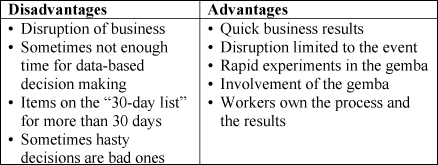
Compared to DMAIC, a kaizen workshop has a number of disadvantages and advantages as listed in the table on the right. One challenge of kaizen workshops is managing the activities before and after the event. Some organizations prepare for a month before a workshop and then have a month of work after the workshop. However, it is fairly common for items on the “30-day list” to be on the list for more than 30 days.

See 5 Whys, 5S, A3 Report, DMAIC, gemba, kaikaku, kaizen, lean thinking.

kanban – A lean signaling tool developed by Toyota that indicates the need for materials or production.

Kanban is the Japanese word for sign, signboard, card, instruction card, visible record, doorplate, or poster. In manufacturing, a kanban is usually a card, cart, or container. A kanban square is a rectangle marked with tape on a table or on the floor. A kanban card is often attached to a storage and transport container. Ideally, kanban signals are physical in nature (containers, cards, etc.), but they can also take the form of a fax (a faxban), an e-mail, or even a computer report.

A kanban signal comes from the customer (downstream) workcenter and gives a workcenter authority to start work. If a workcenter does not have a kanban signal such as a card, container, or fax, it is blocked from doing any more work. For example, when a kanban square is full, the workcenter is not allowed to produce any more.

A kanban system was formerly called a “just-in-time” system because production is done just before the need of a downstream workcenter. However, the term “just-in-time” and the related JIT acronym have fallen out of favor in North America.

A kanban system is a “pull system” because the kanban signal is used to “pull” materials from upstream (supplier) workcenters. In contrast, an MRP system (or any schedule-based system) is a push system. Push systems use a detailed production schedule for each part. Parts are “pushed” to the next production stage as required by the schedule.

Push systems, such as MRP, require demand forecasts and estimated production leadtimes. To be “safe,” most firms use planned leadtimes that are much longer than the average actual time. Unfortunately, long planned leadtimes invariably result in poor forecasts, which result in excess inventory and long actual leadtimes. Long actual leadtimes drive management to further increase leadtimes and compound the problem. Pull systems tend to work better than push systems for repetitive manufacturing as long as the demand is relatively level and cycle times are small.

Toyota uses a dual-card kanban system with two main types of kanban cards – the production kanban and the withdrawal kanban. The production kanban signals (indicates) the need to produce more parts. No parts may be produced without a production kanban. If no production kanban cards are at the workcenter, the workcenter must remain idle and workers perform other duties. Containers for each specific part are standardized, and they are always filled with the same (ideally, small) quantity. The withdrawal kanban signals (indicates) the need to withdraw parts from one workcenter and deliver them to the next workcenter.

The number of kanban cards between two workcenters determines the maximum amount of work-in-process inventory between them. Production must stop if all kanban cards are attached to full containers. When a kanban card is removed, the maximum level of work-in-process inventory is reduced. Removing kanban cards can continue until a shortage of materials occurs. A shortage indicates a problem that was previously hidden by excessive inventory. Once the problem is found, corrective action is taken so the system can function at a lower level of work-in-process inventory.

According to http://en.wikipedia.org/wiki/Kanban, the kanji characters for kanban are .

See blocking, CONWIP, faxban, heijunka, Just-in-Time (JIT), lean thinking, POLCA (Paired-cell Overlapping Loops of Cards with Authorization), pull system, standard products, starving, upstream.

Kano Analysis – A quality measurement tool used to categorize and prioritize customer requirements based on their impact on customer satisfaction; also called the Kano Model, Kano Diagram, and Kano Questionnaire.

Kano Analysis was developed by the Japanese quality expert Dr. Noriaki Kano of Tokyo Rika University to classify customer perceptions of product characteristics. Kano defines five categories of product attributes:

• Must-have attributes (also called must-be or basic/threshold attributes) – The basic functions and features that customers expect of a product or service. For example, an airline that cannot meet airport noise regulations will not succeed in the marketplace.

• Performance attributes (one-dimensional quality attributes) – These attributes result in satisfaction when fulfilled and dissatisfaction when not filled. The better the performance, the greater the customer satisfaction. For example, an airline that provides more entertainment options will be perceived as having better service.

• Delighter attributes (also called attractive quality attributes) – These are the unexpected “extras” that can make a product stand out from the others. For example, an airline that offers free snacks in the waiting area would be a welcome surprise. Delighters vary widely between customers and tend to change over time. This point is consistent with the popular service quality expression, “Today’s delight is tomorrow’s expectation.”

• Indifferent attributes (reverse quality attributes) – These attributes do not affect customer satisfaction.

For example, when customers pick up rental cars at an airport, they will likely have different attitudes about seats, checkout speed, and global positioning systems. Customers will always expect seats in the car and will be completely dissatisfied with a car without seats. Seats, therefore, are a must-have feature. Customers expect the check-in process to take about 15 minutes, but are happier if it takes only 10 minutes. Satisfaction, therefore, increases with check-in speed. Lastly, many customers are delighted if their rental cars have a Global Positioning System (GPS). A GPS, therefore, is a “delighter” feature.

Kano Diagram

Kano Analysis uses a graphical approach as shown in the Kano Diagram on the right. The x-axis (“dysfunctional/functional”) of the diagram measures the level of a particular product attribute (i.e., checkout speed) and the y-axis (“delight/dissatisfaction”) measures customer satisfaction. For example, checkout speed is a performance attribute and is drawn as a 45-degree straight line. Must-have features (e.g., seats) are drawn so that high functionality brings satisfaction up to zero. When a “delighter” feature (e.g., a GPS) is not present, satisfaction is still at or above zero, but increasing a “delighter” can increase satisfaction significantly.

Kano Analysis begins by identifying all possible customer requirements and uses a survey to measure customer perceptions about each requirement. The following is a simple example of a Kano Questionnaire:

Kano questionnaire example

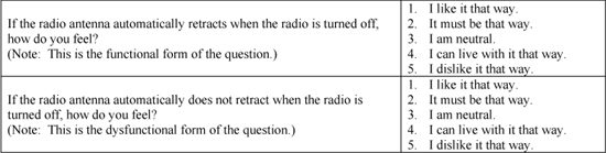
Each question has two parts (1) “How do you feel if that feature is present in the product?” and (2) “How do you feel if that feature is not present in the product?” The responses for the two questions are then translated into curves on the graph.

A Kano Analysis can be used to classify and prioritize customer needs. This is useful because customer needs are not all the same, do not all have the same importance, and are different for different subpopulations. The results of a Kano Analysis can be used to identify customer segments, prioritize customer segments, design products for each segment, and guide process improvement efforts.

Walden et al. (1993) have written a good review article on Kano Analysis.

See Analytic Hierarchy Process (AHP), ideation, New Product Development (NPD), Pugh Matrix, service quality, voice of the customer (VOC).

keiretsu – A Japanese term for a set of companies with interlocking business relationships and shareholdings.

The big six keiretsu are Mitsui, Mitsubishi, Sumitomo, Fuyo (formed primarily from the old Yasuda zaibatsu), Sanwa, and Dai-Ichi Kangyo. The keiretsu were established after World War II, following the dissolution of the family-owned conglomerates known as zaibatsu by the American Occupation authorities. It was the belief of many Americans that they could hasten the spread of democracy in Japan by reducing the concentration of wealth and hence economic power. Shares of companies owned by the zaibatsu were distributed to employees and local residents. As a result that when the stock market reopened in 1949, 70 percent of all listed shares were held by individuals.

Unfortunately, the zaibatsu dissolution was done in a haphazard manner. Often a single factory that merely assembled products for its group became an independent company, lacking a finance department, marketing department, or even a procurement department. To deal with this precarious situation, companies within the former zaibatsu banded together through a system of cross-shareholding, whereby each company owned shares in all other group members’ companies. Within this structure, the major shareholders tended to be banks, a general trading company, and a life insurance company. Today, the “Big Six” keiretsu are all led by their respective banks, which are the largest in Japan.

Because listed companies bought and held onto shares in other listed companies, the ratio of shares owned by individuals in Japan steadily declined to around 20 percent by 2003. There has also never been a hostile takeover of a listed Japanese company, simply because its shareholders have refused to sell at any price. This has made management rather complacent and has greatly reduced shareholders’ rights. Annual shareholders’ meetings in Japan tend to be held on the exact same day, and usually end quickly without any questions.

In the 1990s, when the Japanese stock market was in decline, stable shareholding began to decline. Banks needed to sell their shareholdings to realize gains to cover their credit costs. Life insurers had to sell to realize higher returns to pay their policyholders.

The keiretsu concept is rarely used by Western companies. One exception is the venture capital firm of Kleiner, Perkins, Caufield & Byers, which encourages transactions among companies in which it holds a stake.

See Just-in-Time, lean thinking, Toyota Production System (TPS).

Kepner-Tregoe Model – A systematic scoring approach used to evaluate alternatives in a decision-making process and win organizational approval for the decisions that come out of the process.

The Kepner-Tregoe (KT) Model was developed by Charles H. Kepner and Benjamin B. Tregoe in the 1960s. KT is particularly effective when the organization has to evaluate a number of qualitative issues that have significant trade-offs between them. The KT Model has been “discovered” by many people and is very similar to Criteria Based Matrix, Pugh Matrix, Multi-Attribute Utility Theory (MAUT), and other methodologies.

The steps in the Kepner-Tregoe methodology are:

1. Clearly define the problem at a high level.

2. Establish strategic requirements (musts), operational objectives (wants), and constraints (limits).

3. Rank objectives and assign relative weights.

4. Generate alternatives.

5. Assign a relative score for each alternative on an objective-by-objective basis.

6. Calculate the weighted score for each alternative and identify the top two or three alternatives.

7. List adverse consequences for each top alternative and evaluate the probability (high, medium, low) and severity (high, medium, low).

8. Make a final, single choice between the top alternatives.

The Kepner-Tregoe entry in Wikipedia provides a paired-comparison approach for developing the weights for the KT Model. Each of the criteria is listed on both the columns and the rows. Experts are then asked to independently compare all pairs of criteria in the matrix and to put a “1” when the row criterion is more important than the column criterion. Ties are not allowed. The main diagonal of the matrix is filled with all “1”s. The rows are then summed and divided by the sum of the values in the matrix, which will always be s = n + n(n − 1)/2, where n is the number of criteria that are evaluated.

For example, a location decision has three criteria: cost, distance to markets, and availability of suppliers. The matrix is fort his example is shown below.

Kepner-Tregoe paired-comparison example

For the above analysis, n = 3, which means that s = n + n(n − 1)/2 = 6. This is a good check to help avoid data entry errors. It can be seen in this analysis that the cost dimension clearly dominates the other two criteria. This matrix is only used to compute the weights for the criteria that are used for inputs to the KT Model.

The following is a simple example of the KT Model used for a new plant location decision where management has collected both quantitative and qualitative data, and needs to make difficult decisions regarding trade-offs between costs, risks, quality, etc. All dimensions are scored on a 10-point scale, where 10 is very desirable and 1 is very undesirable. (The values in this table are completely hypothetical.) Of course, many other criteria could also be used in this analysis and a much more detailed cost model should be used to support this type of decision. Many factors such as risk are hard to quantify in the cost model. In this example, China has better cost, but Mexico has better (shorter) distance to makets and greater availability of suppliers. The Mexico site, therefore, appears to be slightly more desirable.

Kepner-Tregoe example

^a Reverse scaled so that 1 is good and 10 is bad.

The final weighted score seldom “makes” the final decision. The scoring process informs the process and helps stimulate a useful debate that supports the final decision, which must be made (and owned) by the management team. It is wise to ask the people who make the decision to create the weights and score the alternatives so they “own” the inputs as well as the results.

Some have criticized the KT Model because it does not explicitly consider risk and uncertainty issues. It is a good practice to include a risk dimension as one of the qualitative factors. In addition, KT tends to focus on consensus, which can lead to group-think and limit creative and contradictory points of view.

The Kepner-Tregoe consulting firm’s website is www.kepner-tregoe.com.

See affinity diagram, Analytic Hierarchy Process (AHP), C&E Matrix, decision tree, facility location, force field analysis, Nominal Group Technique (NGT), Pugh Matrix, TRIZ.

Key Performance Indicator (KPI) – A metric of strategic importance.

See balanced scorecard, dashboard, Key Process Output Variable (KPOV), operations performance metrics.

Key Process Input Variable (KPIV) – See Key Process Output Variable (KPOV).

Key Process Output Variable (KPOV) – A term commonly used in lean sigma programs to describe an important output variable controlled by one or more Key Process Input Variables (KPIVs); also called Critical to Quality (CTQ).

All processes have both inputs and outputs. KPIVs include both controlled and uncontrolled variables. Organizations can change controlled input variables, but cannot change the uncontrolled variables. An example of a controlled input variable is the temperature of an oven; an example of an uncontrolled input variable may be the humidity of the room. Many uncontrolled KPIVs can become controlled if the organization decides to make the investment. For example, room humidity can be controlled with an investment in humidity control equipment.

Key Process Output Variables (KPOVs) are variables that are affected by the KPIVs. KPOVs are usually variables that either internal or external customers care about, such as units produced per hour, defects per million opportunities, and customer satisfaction.

See C&E Matrix, Critical to Quality (CTQ), Key Performance Indicator (KPI), lean sigma.

kickback – See bribe.

kiosk – A small store located in the common area of an enclosed mall or in a larger store.

KISS principle – The acronym “Keep It Simple Stupid,” used to admonish people to eliminate unnecessary complexity.

Wikipedia suggests the more polite version “Keep It Short and Simple.”

See lean thinking, Occam’s razor.

kitting – The manufacturing practice of gathering items for assembly or distribution, typically in boxes or bags.

Kitting is often a good way to ensure that all parts are available and easy to reach. In a manufacturing context, kits of parts are often put together in boxes and given to workers to assemble. In a distribution context, kits are prepared to be packed and shipped. If inventoried, kits should have their own part numbers.

Some consultants argue that kitting is a bad idea because it tends to increase inventory, increase cycle times, and is often a non-value-added step in a process. They advocate that firms should have logical kitting, where they use their MRP systems to ensure that all parts are available. Staging is a similar idea.

See knock-down kit, Materials Requirements Planning (MRP), staging.

KJ Method – A technique for building affinity diagrams named after Kawakita Jiro; also known as KJ Analysis.

The key principle of the KJ Method is that everyone works together in silence to allow for individual creativity and to keep focused on the problem rather than getting sidetracked in discussion. The Nominal Group Technique (NGT) entry includes most of the main ideas for both affinity diagrams and the KJ Method.

See affinity diagram, Nominal Group Technique (NGT).

knapsack problem – An important operations research problem that derives its name from the problem of finding the best set of items that can fit into a knapsack (backpack).

The knapsack problem is to select the items to put into a knapsack (known as a backpack to most students today) that will maximize the total value subject to the constraint that the items must fit into the knapsack with respect to the knapsack’s maximum weight or volume. The knapsack problem is a one of the best-known combinatorial optimization problem in operations research.

Given a set of n items that each have value v_i and weight (or volume) w_i, the knapsack problem is to find the combination of items that will fit into the knapsack to maximize the total value. Stated mathematically, the knapsack problem is to maximize the total value, , subject to the constraint that the items fit into the knapsack, i.e., , where W is the maximum weight (or volume) for the knapsack, and the decision variables x_i are restricted to either zero or one (i.e., x_i {0, 1} for all _i). The “bounded knapsack problem” allows for up to c_i copies of each item. The mathematical statement of the problem is the same except that the domain for the decision variables changes to x_i {0, 1,... , c_i}. The “unbounded knapsack problem” places no upper bound on the number of copies for each kind of item.

The knapsack problem can be solved to optimality with dynamic programming. Although no polynomial-time algorithm is known, fairly large knapsack problems can be solved to optimality quickly on a computer.

See algorithm, integer programming (IP), operations research (OR).

knock-down kit – A kit or box of parts that can be used to assemble a product; also known as Complete Knocked Down (CKD) or Semi-Knocked Down (SKD).

Knock-down kits are commonly used in the automotive industry. The manufacturer sells knock-down kits to a foreign affiliate to avoid paying import taxes or to receive tax preferences for having higher local content. For example, the General Motors factory in northern Hungary received knock-down kits in large wooden boxes from Opal in Germany and assembled them into cars using Hungarian workers. The automobiles assembled in this plant had sufficient local labor content to qualify for tax advantages from the Hungarian government²⁶.

See kitting.

knowledge capital – See knowledge management.

knowledge management – Practices and systems used by organizations to identify, create, represent, and distribute knowledge for reuse, awareness, and learning across the organization.

Hansen, Nohria, and Tierney (1999) defined two knowledge management strategies:

Codification strategy – In some organizations, knowledge management centers on the computer. Knowledge is carefully codified and stored in databases where it can be accessed and used easily by anyone in the company. This is called a codification strategy.

Personalization strategy – In other organizations, knowledge is closely tied to the person who developed it and is shared mainly through direct person-to-person contact. The purpose of the computer for these companies is to help people communicate knowledge, not just store it. This is called the personalization strategy.

A good information systems infrastructure is an important success factor for a good knowledge management system. However, the biggest problem in knowledge management is usually not the information system, but rather the lack of proper incentives for people to add knowledge to the knowledge database. People are busy and often do not have time to add new information that might be valuable to others. Some people are also concerned that if they put their private information into the knowledge management system, their jobs could be at risk and they might, in fact, diminish their value to the firm.

See business intelligence, call center, expert system, help desk, intellectual capital, intellectual property (IP), knowledge capital, knowledge worker, learning organization, Product Data Management (PDM), technology transfer, tribal knowledge.

knowledge work – Jobs that deal primarily with transforming information.

See knowledge worker.

knowledge worker – A person whose primary job is to use his or her intellectual capability with supporting information systems to acquire, accumulate, process, analyze, synthesize, create, develop, use, manage, distribute, and communicate information.

The term “knowledge worker” was first used by Peter Drucker in his book Landmarks of Tomorrow (1959) to describe workers who use their intellectual capacities rather than their manual or physical skills. Knowledge workers are typically involved in tasks such as planning, acquiring, searching, analyzing, organizing, storing, programming, distributing, marketing, or otherwise adding value by transforming information into more valuable information. Knowledge workers include those with information intensive jobs, such as lawyers, scientists, academics, teachers, engineers, medical professionals, programmers, systems analysts, writers, and reporters.

See knowledge management, knowledge work, personal operations management.

Kolmogorov-Smirnov test (KS test) – A non-parametric statistical test that is usually used to determine if a set of observations differs from a hypothesized continuous probability distribution.

The KS test can be used to determine if a particular continuous theoretical distribution (such as the uniform, normal, lognormal, exponential, Erlang, gamma, beta, or Weibull) is a good fit with the data. The KS test compares the empirical cumulative distribution with the hypothesized cumulative distribution function. More generally, the KS test can be used to determine if any two datasets differ significantly without any assumptions about the distribution of data.

The KS test is based on the largest “error” between the actual and theoretical cumulative distribution functions. Given n independent samples arranged in numerical order x₁ x₂ ... x_n, define F_s(x) as the cumulative distribution for the sample. F_s(x_j) = (j+1)/n, therefore, is the fraction of the n observations that are less than or equal to x. Define F(x) as the hypothesized theoretical cumulative distribution. The “one-sided” KS statistics are then D_n⁺ = max(F_s(x_j) − F(x_j)) and D_n⁻ = max(F(x_j) − F_s (x_j)).

Critical values for the D_n statistic are tabulated in many statistics textbooks and are available in many statistical software packages. Unfortunately, Excel does not support the KS test without add-in software, such as Crystal Ball. For large sample sizes, .

Technically, the KS test is only appropriate when all parameters of the distribution are known with certainty. However, in nearly all cases, it is necessary to estimate the parameters from the data. The chi-square test is more appropriate than the KS test for discrete distributions.

Failure to reject the null hypothesis of no difference should not be interpreted as “accepting the null hypothesis.” For smaller sample sizes, goodness-of-fit tests are not very powerful and will only detect major differences. On the other hand, for a larger sample size, these tests will almost always reject the null hypothesis because it is almost never exactly true. As Law and Kelton (2002) stated, “This is an unfortunate property of these tests, since it is usually sufficient to have a distribution that is nearly correct.”

The KS test was developed by Russian mathematicians Andrey Nikolaevich Kolmogorov 1903-1987) and Vladimir Ivanovich Smirnov (, 1887-1974).

See chi-square goodness of fit test.

KPI – See Key Performance Indicator (KPI).

KPOV – See Key Process Output Variable (KPOV).

kurtosis – A statistical measure of the “peakedness” of a probability distribution.

Higher kurtosis means more of the variance is the result of infrequent extreme deviations, as opposed to frequent modestly sized deviations. The sample kurtosis is , where and and where x_i is the i-th value, is the sample mean, m₂ is the second sample moment about the mean (the sample variance), and m₄ is the fourth sample moment about the mean. The Excel KURT function uses the equation , which is an unbiased estimator.

See mean, skewness, variance.

L

labor grade – A classification system that groups jobs together that have approximately the same market value; also called pay grade or job class.

Labor grades are usually based on skills, experience, education, duties, budget responsibilities, level of independence, or leadership responsibilities and indicate pay ranges.

See human resources, job design, pay for skill.

labor intensive – An adjective used to describe products or services that require significant labor time and cost but relatively little capital.

Examples of labor intensive businesses include consulting, accounting, barber shops, teaching, and call centers. Labor intensive products and services are sometimes good candidates for outsourcing to lower labor cost economies. In some situations, labor intensive processes can be automated to reduce unit cost and improve quality, but often at the expense of more capital, higher fixed costs, and less flexibility.

See automation, capital intensive, outsourcing, service management, value added ratio.

labor management systems – See work measurement.

labor standards – See work measurement.

lagging indicator – See leading indicator.

LAI – See Lean Advancement Initiative (LAI).

landed cost – An inventory costing term for the actual or standard procurement, transportation, duties, taxes, broker fees, and other costs required to “land” a product at a location.

The term “landed cost” is usually used in the context of an imported purchased item.

See logistics, offshoring, outsourcing.

Last-In-First-Out (LIFO) – (1) In an inventory management or queue management context: A priority rule based on the last arriving item, unit, or customer. (2) In an accounting context: A method for assigning costs based on the cost for the most recently manufactured or purchased items.

In inventory management with LIFO, the last unit put into inventory (or queue) will be the first to go out. This practice can result in some inventory being in inventory for a long time. In contrast, with First-In-First-Out (FIFO), the first unit put into the inventory will be the first to go out. The same statements are true in the context of a queue discipline. With the LIFO queue discipline, the last arriving customer is serviced first.

In accounting, LIFO is used to determine the cost of goods sold where the most recent units purchased from suppliers are assumed to be sold first. Most U.S.-based companies use LIFO to reduce income tax in times of inflation.

Note that inventory management and accounting policies can be different. It is quite common for the warehouse to use FIFO to manage inventory, where the accounting system uses LIFO to assign costs.

See cost of goods sold, dispatching rules, First-in-First-Out (FIFO), inventory valuation, queuing theory.

late configuration – See postponement.

late customization – See postponement.

lateness – See service level.

Law of Large Numbers – A fundamental concept in probability and statistics that describes how the average of a randomly selected sample from a large population is likely to grow closer to the true average of the whole population as the number of observations increases.

For example, the average weight of 10 apples randomly selected from a barrel of 100 apples is probably closer to the true average weight of all 100 apples than the average weight of 3 apples taken from that same barrel.

The weak Law of Large Numbers states that as the sample size grows larger, the difference between the sample mean and the population mean will approach zero. The strong Law of Large Numbers states that as the sample size grows larger, the probability that the sample and population means will be equal approaches one.

One of the most important conclusions of the Law of Large Numbers is the Central Limit Theorem, which describes how sample means tend to occur in a normal distribution around the mean of the population regardless of the shape of the population distribution, especially as sample sizes get larger.

See Central Limit Theorem

layout – See facility layout.

LCL (less than container load) – See less than container load (LCL).

leading indicator – A variable that changes in advance of a new trend or condition and therefore can be used to predict another variable one or more periods ahead.

Examples of leading indicators include economic variables, such as the number of building permits, non-residential housing, mobile phones shipped, unemployment insurance claims, money supply, and inventory changes. Policy makers often watch many of these leading indicators to decide what to do about interest rates.

In contrast, coincident indicators change at the same time as the variable of interest and lagging indicators change after the variable of interest. These variables, therefore, are of no use for predictive purposes, but can sometimes confirm the existence of a condition or trend.

See balanced scorecard, econometric forecasting, forecasting.

leadtime – The planned replenishment time for an order; often written as two words (lead time); also called production leadtime, manufacturing leadtime, and planned leadtime.

The planned leadtime is a planning factor used in both MRP and reorder point systems for the planned time required to replenish inventory from a supplier (a purchase order) or from a plant (a manufacturing order). This planning factor is called the “replenishment leadtime” in SAP.

Ideally, the planned leadtime is a reliable forecast of the expected (average) actual replenishment time in the future. In other words, the planned leadtime should not include any cushion or buffer to handle situations where the actual leadtime is longer than average. The buffer should be handled by the safety stock and should not be imbedded in the planned leadtime.

The planned leadtime for a manufacturing order is the sum of the planned leadtimes for all steps in the routing for the order. For each operation, this typically includes (a) the queue time before the operation begins, (b) the setup time to get the machine ready for production, (c) the run time to process the order, and finally (d) the post-operation time to wait for the order to be picked up and moved to the next workcenter.

The term “leadtime” is often used as a synonym for throughput time, cycle time, flow time, and customer leadtime. However, the prefix “lead” suggests that the term “leadtime” should be used primarily as a planning factor for the time to “lead” the event rather than as the actual throughput time. It is better, therefore, to use the terms “throughput time,” “cycle time,” or “flow time” rather than “leadtime” when describing actual throughput times. (See the cycle time entry to better understand the two conflicting definitions of cycle time.)

The planned leadtime is a constant, but the actual throughput time (sometimes called cycle time) is a random variable and has a minimum, maximum, mean, standard deviation, median, etc. Note that the safety stock calculation should use either an estimate of the longest leadtime or the more complicated safety stock equation that includes both the mean and standard deviation of the leadtime. (See the safety stock entry for more detail.)

The promised customer leadtime is the promised customer wait time for an order. The actual customer leadtime is the actual wait time (a random variable) experienced by the customer.

It is important to understand that the planned leadtime, actual leadtime (throughput time, flow time), promised customer leadtime, and actual customer leadtime might all be different. Therefore, it is important for managers, engineers, and students of operations management to be very clear when they use these terms. When a manager reports that the factory has a leadtime of two weeks, this could mean a two-week planned leadtime, two-week average leadtime, two-week minimum leadtime, two-week modal leadtime, two-week promised customer leadtime, etc.

The cycle time entry provides more insights into these and other closely related issues.

See cumulative leadtime, customer leadtime, cycle time, demand during leadtime, leadtime syndrome, manufacturing order, purchase order (PO), purchasing, purchasing leadtime, push-pull boundary, reorder point, routing, run time, takt time, time in system, turnaround time.

leadtime syndrome – A vicious cycle where a supplier’s quoted leadtime gets longer, which results in customers ordering more to cover their planned leadtime, which results in the supplier quoting an even longer leadtime.

The cycle can be described as follows:

1. A manufacturer increases the quoted leadtime. This could be for any reason, such as a vacation, a machine problem, a slight increase in demand, etc.

2. The customer learns about the increased leadtime and releases orders earlier to cover the demand during the planned leadtime. Note that the customer’s true average demand did not change in this scenario.

3. The manufacturer receives the larger order, adds it to the order backlog, and further increases the quoted leadtime. The leadtime syndrome continues back to step 1.

The solution to the leadtime syndrome is for customers to communicate their true demand to their suppliers to give their suppliers forward visibility of their true demand and for suppliers to avoid increasing quoted leadtimes, even when the demand increases. The leadtime syndrome is closely related to the bullwhip effect. George Plossl (1985) discussed the leadtime syndrome in his books and seminars in the 1980s.

See bullwhip effect, force majeure, leadtime, Parkinson’s Laws.

Lean Advancement Initiative (LAI) – A learning and research community that brings together key aerospace stakeholders from industry, government, and academia; formerly called the Lean Aerospace Initiative.

LAI is a consortium-guided research program headquartered at the Massachusetts Institute of Technology (MIT) Department of Aeronautics and Astronautics, in close collaboration with the Sloan School of Management. LAI is managed under the auspices of the Center for Technology, Policy and Industrial Development, an interdisciplinary research center within the Engineering Systems Division. LAI was born out of practicality and necessity. Declining procurement budgets, rising costs, and overcapacity prompted the defense acquisition strategy to stress affordability rather than just performance at any cost. LAI was formally launched in 1993, when leaders from the U.S. Air Force, MIT, labor unions, and defense aerospace businesses forged a trail-blazing partnership to transform the industry, reinvigorate the workplace, and reinvest in America by applying lean manufacturing principles. Most of the above comes from LAI’s website (http://lean.mit.edu).

See lean thinking.

Lean Aerospace Initiative – See Lean Advancement Initiative (LAI).

lean design – Lean design is a set of tools for reducing the new product development cost and time with a focus on reducing variation, addressing bottlenecks, eliminating rework, and managing capacity.

See lean thinking, New Product Development (NPD).

Lean Enterprise Institute (LEI) – A nonprofit education and research organization founded by Jim Womack in 1997 to promote and advance the principles of lean thinking in every aspect of business and across a wide range of industries.

LEI develops and teaches lean principles, tools, and techniques designed to enable positive change. A major LEI objective is to create a complete toolkit for lean thinkers to use in transforming businesses. The lean toolkit is intended to be a dynamic and continually evolving means of sharing knowledge among lean thinkers. One of the more important publications of the LEI is the Lean Lexicon, edited by Chet Marchwinski and John Shook (2009). The LEI website is www.lean.org.

See 8 wastes, lean thinking.

lean manufacturing – See lean thinking.

lean production office – See lean promotion office.

lean promotion office – The program “office” (team) that manages the lean implementation.

This team provides leadership, training, and support for implementing a lean manufacturing program.

See lean thinking, program management office.

lean sigma – A formal process improvement program that combines six sigma and lean thinking principles; also called lean six sigma.

Six sigma versus lean – Lean sigma process improvement programs are widely used in larger firms throughout North America and Europe. These programs grew out of the six sigma program, which was developed by Motorola and expanded and popularized by GE. In recent years, nearly all six sigma programs have changed their names to lean sigma to reflect the fact that they now embrace many lean principles and tools. The George Group, a North American consultancy that owns the trademark to the name “lean sigma,” argues that six sigma programs historically focused on reducing variation, whereas lean programs focused on reducing the average cycle time (George, Rowlands, & Kastle 2003; George 2003). However, this dichotomy is too simplistic given that many organizations use six sigma tools, such as process mapping, to reduce the average cycle time and waste and many organizations use lean principles, such as error proofing and small lotsizes, to reduce variation and defects. Clearly, both lean and six sigma seek to reduce variation, defects, waste, and cycle time.

How to combine six sigma and lean – Paul Husby, retired senior vice president at 3M, and other thought leaders have argued that six sigma tends to rely on statistical methods, whereas lean is more of a philosophy of how a firm should be managed, with emphasis on simplicity, visibility, standardized work, and accountability. He suggests the following simple rule: If the cause is unknown or difficult to determine, use the six sigma DMAIC approach, but otherwise use lean.

According to Scot Webster, former vice president of Quality and Supply Chain at Medtronic²⁷, “Six sigma makes a science of process capability and lean makes a science of process flow and both are implemented with the DMAIC approach.” Webster argued that the standard six sigma equation Y = f (x₁, x₂, ... , x_N) works for both six sigma and for lean. The only difference is that for six sigma, the challenge is to find the vital few x_i variables among a large number of possible variables; for lean, the challenge is to find the vital few from only 18 potential tools. He listed 11 of the 18 tools in his publicly available talk: transfer lot size, process lot size, options, rework, downtime, external set up, internal set up, attended machine, unattended machine, move, and labor. He summarized his talk on lean sigma by arguing that both six sigma and lean are about leadership development and asserted that lean sigma was 70 percent leadership development and 30 percent process improvement.

One of the best ways to combine lean and six sigma principles in a lean sigma program is to use the six sigma program framework to provide an organizational structure for process improvement projects. This structure helps the firm align projects with the organization’s strategies and goals, staff appropriately, and have proper accountability. Many six sigma projects use lean manufacturing principles and tools (cycle time reduction, lotsize reduction, etc.). The six sigma DMAIC approach can be used for all projects, but experts such as Husby argue that DMAIC is not needed for most lean projects because the problem and the solution are already well understood.

Five views of lean sigma – Zhang, Hill, and Gilbreath (2010) identify five different views of lean sigma programs as shown in the figure on the right. From the metric point of view, lean sigma is about maximizing the “sigma level” (minimizing the defect rate or some other process capabilities metrics), often with the target of six sigma (or 3.4 defects per million opportunities). From the tool point of view, lean sigma is about applying managerial tools (e.g., brainstorming) and statistical tools (e.g., design of experiments) to problem solving. From the project point of view, lean sigma is about defining and executing lean sigma projects with black belt or green belt project leaders using the DMAIC five-step problem solving methodology. From the program point of view, lean sigma is about a program management office that finds and prioritizes problems that need to be addressed and then charters and resources projects to address those problems. From the philosophy point of view, lean sigma is about building a sustainable culture of leaders who are relentless about continuously improving processes to eliminate waste and defect.

Source: Professor Arthur V. Hill

DMAIC – Lean sigma projects often use the six sigma five-step process called DMAIC – Define, Measure, Analyze, Improve, and Control. These five steps are described in more detail in the DMAIC entry. Lean sigma projects are often driven by an understanding of the “entitlement” (i.e., the best possible performance) for a process. However, the target may be different from the entitlement.

Key roles in a lean sigma program – Lean sigma identifies five key roles for its successful implementation (Harry & Schroeder 2000). Certification programs for most of these roles are available from many sources. Some of the content below is adapted from the ASQ.org site. The executive leadership and champion work at the program level, whereas master black belts, black belts, green belts, and yellow belts work at the project level.

• Executive Leadership: Provide overall leadership for the program office by aligning lean sigma projects with corporate and business unit strategies. They also ensure that proper resources are allocated to the program. The leadership should include the CEO and other key top executives. They are responsible for setting the vision for the lean sigma program. They also empower the other role holders with the freedom and resources to explore new ideas for breakthrough improvements.

• Champion: Lead the lean sigma program. The champion is selected by the Executive Leadership and is usually a member of the executive team. The champion must translate the company’s strategies and goals into projects. He or she also identifies resources and removes barriers to program and project success. The champions also acts as a mentor to the master black belts and black belts. At GE, this level of certification is now called Quality Leader. The champion usually manages the project selection process and the project hopper (the set of potential projects) and also selects people to become black belts.

• Master black belts: Assist champions in program management and train and coach black belts and green belts in project management. They are usually full-time resources for the lean sigma program. Master black belts should be experienced black belts.

• Black belts: Lead problem-solving projects and train and coach team members with help from master black belts. Black belts usually have between four and eight weeks of training and are normally assigned to manage projects full-time for a limited period (normally 2-3 years). They focus primarily on lean sigma project execution, whereas champions and master black belts focus on identifying projects.

• Green belts: Assist black belts on black belt projects and lead green belt projects while maintaining full-time job responsibilities. Green belts usually have between two and four weeks of training.

• Yellow belts: Participate as project team members and review process improvements that support the project. Many lean sigma programs do not use this designation.

• White belts: Understand basic lean sigma concepts and work on local problem-solving teams that support overall projects but may not be part of a lean sigma project team. Few programs use this designation.

Lean sigma training programs – The following is a list of topics that are often included in lean sigma training programs. Almost all of these topics can be found in this encyclopedia.

See benchmarking, brainstorming, C&E Diagram, C&E Matrix, Capability Maturity Model (CMM), causal map, champion, control chart, control plan, Critical to Quality (CTQ), cross-functional team, defect, Defects per Million Opportunities (DPMO), Deming’s 14 points, deployment leader, Design for Six Sigma (DFSS), Design of Experiments (DOE), DMAIC, entitlement, external setup, Failure Mode and Effects Analysis (FMEA), Gauge R&R, human resources, impact wheel, implementation, inductive reasoning, ISO 9001:2008, just do it, Key Process Output Variable (KPOV), lean thinking, linear regression, Metrology, PDCA (Plan-Do-Check-Act), post-project review, process, process capability and performance, process improvement program, process map, program management office, project charter, project hopper, Pugh Matrix, quality management, quality trilogy, quick hit, RACI Matrix, sigma level, stage-gate process, stakeholder analysis, Statistical Process Control (SPC), statistical quality control (SQC), strategy map, Taguchi methods, Total Quality Management (TQM), transactional process improvement, value chain, value stream map, voice of the customer (VOC), zero defects.

lean six sigma – See lean sigma.

lean thinking – A philosophy and set of practices originally developed at Toyota that seeks to eliminate waste; also known as lean manufacturing or just lean.

A brief history of lean – Lean concepts were first introduced at Toyota by Taiichi Ohno in Japan (Ohno 1978). Richard Schonberger played an important role in popularizing “just-in-time” (JIT) concepts in the U.S. in the 1980s, which emphasized the material flow aspects of lean (Schonberger 1982, 1986). The term “lean” was coined by John Krafcik²⁸ in the MIT International Motor Vehicles Program, but popularized in the book The Machine That Changed the World (Womack, Jones, & Roos 1991). More recently, Jim Womack at LEI has led a resurgence of interest in lean thinking with a view of lean that goes well beyond materials flow and manufacturing (Womack & Jones 2003). Today, the term “lean thinking” is used to emphasize that lean is more of a philosophy than a set of tools and that lean principles can be applied in services, government, and other non-manufacturing contexts.

Benefits of lean – Lean thinking focuses on reducing waste though a high level of engagement of the people in the “gemba” (the place that real work is done). Many firms that embraced lean thinking have been able to achieve significant benefits, such as reduced cycle time, inventory, defects, waste, and cost while improving quality and customer service and developing workers.

The basic concepts of lean – Many lean experts argue that promoters of lean sigma programs “just don’t get it.” They argue lean sigma programs use some lean tools but miss the lean philosophy, which means they do not truly understand lean. Clearly, lean is much more than a set of tools.

Many lean consultants teach that lean is about simplifying processes, but then over-complicate lean by using too many Japanese words and focusing more on lean tools than on lean philosophy. After 25 years of study, this author believes that lean thinking can be summarized in just five words as shown in the simple diagram below.

Source: Professor Arthur V. Hill

Lean is about making processes simple and visual. Once processes are simple and visual, it becomes easier for people in the “gemba” to make them error-proof and to eliminate waste. Once processes are simple, visual, error-proof, and wasteless, it is important to make them standard so that the benefits are sustainable. Lastly, respect for people before, during, and after the process improvement activity is critical to success.

The house of lean – The popular house of lean figure shown below is often used to teach the fundamentals of lean thinking. A similar figure appears in the Ohno (1978) book. This figure is adapted from Pascal (2002). The left side focuses on managing materials, the right side focuses on managing the manufacturing process, and the bottom focus on the fundamentals. Definitions for the terms in this figure can be found in this encyclopedia.

The house of lean

Lean for process improvement – The “virtuous cycle of lean” is shown in the figure below.

Source: Professor Arthur V. Hill

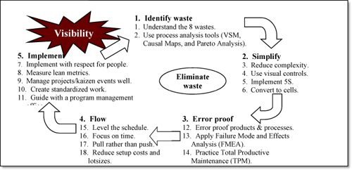
The cycle begins by identifying waste using the 8 wastes framework, value stream mapping, causal maps (or Ishikawa Diagrams), and Pareto Analysis. Once waste has been identified, it is eliminated (or at least reduced) by making the process simpler, more visible, and more error-proof. Flow is then achieved by leveling the schedule, reducing cycle time, using a pull system, and reducing setup costs, setup times, and lotsizes (one-piece flow is the ideal). Finally, implement changes with respect for people (the gemba), focusing on lean metrics, such as the value added ratio, using well-executed kaizen events, and creating standardized work, all guided by a strong program management office. The virtuous cycle is self-reinforcing because the new improvement process will be even more visible, which makes it easier to see and eliminate waste. This figure was developed by this author and has been validated from first-hand experience with many factory and hospital lean implementations.

Spear and Bowen’s five rules – Spear and Bowen (1999) defined five rules that capture much of the lean philosophy at Toyota. They emphasized that lean is more of a philosophy than a set of tools. These four rules are briefly described as follows:

• Rule 1. Specifications document all work processes and include content, sequence, timing, and outcome – Each process should be clearly specified with detailed work instructions. For example, when workers install seats with four bolts, the bolts are inserted and tightened in a set sequence. Every worker installs them the same way every time. While lean thinking shows respect for people and values experimentation (using PDCA), individual workers do not change processes. Teams work together to experiment, analyze, and change processes. Workers need problem-solving skills to their support teams in improving standard processes over time.

• Rule 2. Connections with clear yes/no signals directly link every customer and supplier – Lean uses kanban containers (or squares) that customers use to signal the need for materials movements or production.

• Rule 3. Every product and service travels through a single, simple, and direct flow path – Toyota’s U-shaped workcells are the ultimate manifestation of this rule. This improves consistency, makes trouble shooting easier, and simplifies material handling and scheduling.

• Rule 4. Workers at the lowest feasible level, guided by a teacher (Sensei), improve their own work processes using scientific methods – Rule 4 is closely tied with Rule 1 and engages the entire workforce in the improvement efforts.

• Rule 5. Integrated failure tests automatically signal deviations for every activity, connection, and flow path – This is the concept of jidoka or autonomation. It prevents products with unacceptable quality from continuing in the process. Examples include detectors for missing components, automatic gauges that check each part, and visual alarms for low inventory. The andon light is a good example of this rule.

See 3Gs, 5S, 8 wastes, A3 Report, absorption costing, agile manufacturing, agile software development, andon light, batch-and-queue, blocking, Capability Maturity Model (CMM), catchball, cellular manufacturing, champion, continuous flow, cross-training, defect, demand flow, Drum-Buffer-Rope (DBR), facility layout, flow, functional silo, gemba, heijunka, hidden factory, hoshin planning, ISO 9001:2008, jidoka, JIT II, job design, Just-in-Time (JIT), kaizen, kaizen workshop, kanban, Keiretsu, KISS Principle, Lean Advancement Initiative (LAI), lean design, Lean Enterprise Institute (LEI), lean promotion office, lean sigma, milk run, muda, multiplication principle, one-piece flow, Overall Equipment Effectiveness (OEE), overhead, pacemaker, pitch, process, process improvement program, program management office, project charter, pull system, Quick Response Manufacturing, red tag, rework, scrum, sensei, Shingo Prize, Single Minute Exchange of Dies (SMED), stakeholder analysis, standardized work, subtraction principle, supermarket, takt time, Theory of Constraints (TOC), Toyota Production System (TPS), transactional process improvement, true north, two-bin system, value added ratio, value stream, value stream manager, value stream map, visual control, waste walk, water spider, zero inventory.

learning curve – A mathematical model that relates a performance variable (such as cost per unit) to the number of units produced, where the performance variable decreases as the cumulative production increases, but decreases at a slower rate; also called experience curve.

All systems can improve over time, and the rate of improvement can and should be measured. This learning can take place at any level: the machine, individual, department, plant, business unit, and firm. Some authors use the term “experience curve” for more complex systems, such as factories or firms; however, there is no practical difference between the learning curve and experience curve concepts.

The performance variable is usually the cost per unit or time per unit, but could be any variable that has an ideal point of zero. For example, other possible variables could be the defect rate (defects per million opportunities, DPMO), customer leadtime, etc. Variables, such as yield and productivity, are not appropriate performance variables for the learning curve because they do not have an ideal point of zero.

The graph below is an example of a learning curve with k = 80%, y₁ = 100, and a learning parameter of b = 0.322. Learning curve graphs are only defined for integer values of n.

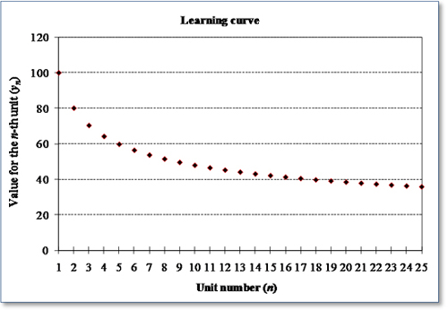
“Satisficing” is the practice of meeting the minimum requirements rather than seeking to improve over time. People tend to “satisfice” if not given an appropriate goal. The learning curve, therefore, can be used to set appropriate goals for improvement. The learning rate can also be used to benchmark organizational learning across organizational boundaries. Every measure in a balanced scorecard could have a complementary measure for its rate of learning.

With the learning curve, every time the cumulative production volume doubles, the cost goes down by a fixed percentage. (The remainder of this discussion will assume that the performance variable is cost.) For example, with an 80% learning curve, the cost goes down by 20% every time the cumulative production doubles. If the unit cost for unit 1 is $100, the unit cost for unit 2 is $80, the unit cost for unit 4 is $64, etc.

The equation for the learning curve model is y_n = y₁n^–b, where n is the unit number, y_n is the cost for the n-th unit, y₁ is the value for the first unit, and b is the learning parameter. The model requires that b 0 and uses a negative sign in the model. Many textbooks present the model without a negative sign and have b 0.

For a k-percent learning curve, the cost goes down by (1−k)% every time the cumulative production doubles. If the learning rate parameter k is known, the learning curve is given by b = −ln(k)/ln(2). Conversely, if the learning parameter b is known, the learning rate parameter is k = 2^–b.

For example, for an 80% learning curve, k = 0.8 and b = 0.322. With y₁ = 100, the unit cost for the first 8 units is 100, 80, 70, 64, 60, 56, 53, and 51. (Note that these values are rounded to the nearest integer.)

The cumulative cost through the n-th unit is given by the following approximation (Camm, Evans, & Womer 1987; Badiru 1992): . This approximation was tested for k = 0.8 and was found to have an absolute percentage error of less than 2% when n = 1. The error approaches zero as n increases, with an error of less than 0.03% for n > 100. This equation can be used to estimate the average cost through the n-th unit as A_n = Y_n/n.

The easiest approach for estimating the learning parameter from historical data is to find the value that fits the curve to the first and last observed historical values b = −ln(y_n/y₁)/ln(n). The parameter y₁ for this model is set to the first observed historical value. However, this approach places too much weight on the first and last values and ignores the historical data in between.

Another approach recommended by some is to estimate the model parameters b and y₁ with linear regression on log transformed historical data. We first apply the natural log transform to both sides of the basic learning curve equation to find ln(y_n) = a − bln(n), where a = ln(y₁). We then apply linear regression to the transformed data to estimate the intercept (a = ln(y₁)) and slope (b) for the line. We then estimate the intercept y₁ = exp(a) and learning rate k = 2^−b. However, linear regression poses some serious technical problems due to autocorrelation in the data. Several methods, such as first differences, can be used to try to compensate for the autocorrelation problem, but that is beyond the scope of this document. Note that the required transformation is not possible if the performance variable is zero for any historical observation.

See autocorrelation, balanced scorecard, half-life curve, human resources, learning organization, linear regression, Moore’s Law, operations performance metrics, satisficing, workforce agility.

learning organization – An organization that has the ability to learn from its environment and improve its ability to compete over time.

Most organizations today find that their current products and processes will become obsolete in a fairly short period of time. Jack Welch, former chairman of the board and CEO of General Electric, emphasized this point in his famous quote, “When the rate of change outside the company is greater than the rate of change inside the company, then we are looking at the beginning of the end” (Caroselli 2003, page 137).

It is necessary, therefore, for managers to lead their organizations in such a way that their organizations have built-in systems for improving (learning) over time. Learning organizations have the ability to transform their organizational experiences into improved products, processes, and knowledge.

Organizations can learn from many sources, including:

• Customers – To learn about customer’s needs and desires as they change over time.

• Suppliers – To learn about new materials, technologies, and processes.

• Research labs and technology suppliers – To learn about new product and process technologies being developed by research labs, universities, and suppliers.

• Workers – To document new processes and make tacit knowledge explicit.

Senge (1990) argues that learning organizations exhibit five main characteristics: systems thinking, personal mastery, mental models, a shared vision, and team learning. This author has created the following list of strategies that organizations can deploy to nurture and accelerate learning. Most of these described are described in other entries in this encyclopedia.

• Create knowledge management systems – To leverage information systems to codify and share knowledge.

• Measure learning – To assess and reward learning based on measurable performance improvement. The learning curve and the half-life curve can be used for this.

• Offer service guarantees – To reward customers for sharing their complaint information.

• Pursue early supplier involvement – To get suppliers more involved in product design.

• Benchmark best-in-class processes and products – To capture standards and processes to use as a basis of comparison. See benchmarking.

• Use cross-training, job rotation, job enlargement, and job enrichment to develop workers – To disseminate learning within the firm.

• Use co-location – To improve learning across different functions and firms. See co-location.

• Implement cycle counting – To find the source of data integrity problems. See cycle counting.

• Use post-project reviews – To evaluate what went well (reinforce behavior) and what could have been done better (to identify new behaviors) when a project is completed. See post-project review.

• Conduct root cause analysis after every adverse event – To learn what could have been done to prevent a specific situation with an undesired (or desired) effect. See Root Cause Analysis (RCA).

See balanced scorecard, business intelligence, co-location, cross-training, cycle counting, half-life curve, human resources, intellectual capital, intellectual property (IP), job enlargement, job rotation, knowledge management, learning curve, Moore’s Law, operations performance metrics, post-project review, Root Cause Analysis (RCA), satisficing, workforce agility.

legacy system – An existing computer-based information system that is only being used until a newer system is fully operational.

The term “legacy” often implies that the old system has been in use for a long time and is becoming obsolete. Legacy systems are often expensive to maintain because they are difficult to interface with new systems.

See Enterprise Resources Planning (ERP).

less than container load (LCL) – A shipment of a container that is not full; LCL can also refer to a customer’s freight that is combined with others to produce a full container load.

See less than truck load (LTL), logistics, shipping container, truck load.

less than truck load (LTL) – A shipment that does not fill the truck or a shipment with less than the weight needed to qualify for a truck load quantity discount.

LTL shipments do not qualify for full truck load (FTL) rates based on weight or volume and normally have a longer delivery time due to consolidation with other LTL shipments. LTL is usually used to designate shipments weighing between 100 and 10,000 pounds. These shipments are usually not economical to ship via parcel shippers or FTL carriers and fall somewhere in between. This quantity of freight also involves more intermediate handling than does truck load freight.

A typical LTL carrier collects freight from various shippers, consolidates that freight onto trailers, and sends the shipment for line-haul. For delivery, a similar process is followed, where the freight from the line-haul trailer is unloaded, re-sorted, and sent for delivery. In most cases, drivers make deliveries first and then pick up from shippers once the trailer is empty. Therefore, most pickups are made in the afternoon and most deliveries are performed in the morning.

The main advantage of using an LTL carrier is that a shipment may be transported for a fraction of the cost of hiring an entire truck and trailer for an exclusive shipment. A number of additional services are also available from LTL carriers that are not typically offered by FTL or parcel carriers. These services include liftgate service at pickup or delivery, residential (also known as “non-commercial”) service at pickup or delivery, inside delivery, notification prior to delivery, freeze protection, and others. These services are usually billed at a predetermined flat fee or for a weight-based surcharge calculated as a rate per pound or per hundred-weight.

See carrier, consolidation, cross-docking, less than container load (LCL), logistics, quantity discount, shipping container, trailer, truck load.

level – See bill of material (BOM).

level loading – See load leveling.

level of service – See service level.

level production – See chase strategy, Heijunka, level strategy.

level strategy – A production planning approach that keeps the workforce level constant and satisfies seasonal demand with inventories built during the off season, overtime, or subcontracting.

The level strategy maintains a constant workforce level and meets demand with inventory (built in the off season), overtime production, subcontracting, or some combination thereof. In contrast with a chase strategy, the workforce level is changed to meet (chase) demand.

Many firms are able to economically implement a chase strategy for each product and a level employment overall strategy by offering counter-seasonal products. For example, a company that makes snow skis might also make water skis to maintain a constant workforce without building large inventories in the off season. Other examples of counter-seasonal products include snow blowers and lawn mowers (e.g., Toro) and snowmobiles and all terrain vehicles (e.g., Polaris Industries).

See chase strategy, heijunka, load, load leveling, Master Production Schedule (MPS), production planning, Sales & Operations Planning (S&OP), seasonality, subcontracting.

leverage the spend – Combine purchasing from multiple units in an organization to justify negotiation for lower prices from a supplier.

An organization can “leverage the spend” with a supplier by combining all purchases across multiple departments, plants, and divisions into one negotiated contract. This allows the organization to buy in larger quantities, which gives it the power to bargain for a lower price. One common example is for Maintenance, Repair and Operations (MRO) items (such as office supplies) purchased by a large multi-divisional organization. Many organizations used to allow each department, location, plant, and division to buy its own MRO supplies. The firm can often get a much better price from suppliers by combining “the spend” (all purchases) across all divisions and all departments. The same concept can be used for many direct materials (non-MRO items). Many consulting firms have made this concept a major part of their consulting services.

See consolidation, Maintenance-Repair-Operations (MRO), purchasing, spend analysis, Supply Chain Management.

Lewin/Schein Theory of Change – A three-stage model developed by Kurt Lewin and Edgar Schein that describes how individuals change; the three stages are unfreeze, change, and refreeze.

Kurt Lewin developed a three-stage model of change that has come to be known as the unfreeze-change-refreeze model. Edgar Schein provided further detail for a more comprehensive model of change that he called “cognitive redefinition.” The combined model is often called the Lewin/Schein Theory of Change or the Lewin/Schein Change Model (Schein 1992). The three stages are described briefly below.

Unfreeze (motivate the change) – Change requires adding new forces for change or removing some of the existing factors that are at play in perpetuating the current behavior. This unfreezing process has three sub-processes that relate to a readiness and motivation to change:

• Disconfirmation – Learning and change begins with dissatisfaction or frustration, such as not meeting personal goals.

• Survival anxiety – When people accept the disconfirming information as valid, they feel “survival anxiety” or guilt. However, this may not be sufficient to prompt change if “learning anxiety” is present.

• Psychological safety – Learning anxiety triggers defensiveness and resistance due to the pain of having to unlearn what had been previously accepted. Three stages occur in response to learning anxiety: (1) denial, (2) scapegoating and passing the buck, and (3) maneuvering and bargaining. It is necessary to move past the possible anxieties for change to progress. This can be accomplished by either having the survival anxiety be greater than the learning anxiety or, preferably, by reducing learning anxiety. Change agents can create psychological safety by having people work in groups, providing positive visions for the learner, breaking the learning process into small steps, providing coaching, etc.

Move (change what needs to be changed) – Once sufficient dissatisfaction with the current conditions and a sincere desire to change exists, it is necessary to identify exactly what needs to be changed. Three possible impacts from processing new information are: words take on new or expanded meaning, concepts are interpreted within a broader context, and the scale used to evaluate new input is adjusted. A concise view of the new state is required to clearly identify the gap between the present and proposed state. Activities that aid in making the change include imitation of role models and looking for personalized solutions through trial-and-error learning.

Refreeze (making the change permanent) – Refreezing is the final stage where new behavior becomes habitual, which includes developing a new self-concept and identity and also establishing new interpersonal relationships. In the process improvement program literature, this is called the “control plan.”

The ADKAR model is very similar, but somewhat easier to understand and apply.

See ADKAR Model for Change, change management, control plan, force field analysis.

life cycle cost – See total cost of ownership.

life cycle planning – See product life cycle management.

lifetime demand – See all-time demand.

LIFO – See Last-In-First-Out (LIFO).

Likert scale – A psychometric scale commonly used in survey instruments.

When responding to a Likert-scaled item on a survey, respondents typically specify their level of agreement to a statement. The following is an example of a five-point Likert scale often used by this author and his research colleagues: 1 = Disagree strongly, 2 = Disagree, 3 = Neutral, 4 = Agree, 5 = Agree strongly. Note that each phrase in this scale starts with either Disagree or Agree.

The Likert scale is named after Rensis Likert, who published a report describing its use (Likert 1932). The proper pronunciation is “lick-urt” rather than “lie-kurt.”

line balancing – The problem of assigning tasks to workstations to minimize the number of workstations required while still satisfying the cycle time and precedence constraints.

A perfectly balanced process will have all steps in the process working at exactly the same rate. This will result in no idle time for any step and no inventory between steps. When designing an assembly line, many tasks (elements) need to be assigned to workstations. These assignments are constrained by the cycle time for the line (i.e., one completion every five minutes) and the precedence relationships between the tasks (i.e., some tasks need to be done before others). Many operations researchers have developed sophisticated mathematical computer models to solve this problem. The line balancing problem is less important when the organization can use cross-trained workers who can move between workstations as needed to maximize flow.

See assembly line, cross-training, facility layout.

line extension – A new product that is a variation of an existing product.

Line extensions are not significantly different from the original product and almost always share the same brand. Examples include a new package size, a new flavor, or a new ingredient. For example, Cheerios cereal now comes in many variants, with different flavors and package sizes.

See New Product Development (NPD).

line fill rate – See service level.

line of visibility – The line that separates a service operation into back office operations (that take place without the customer) and front office operations (that are in direct contact with the customer).

See back office, service blueprinting, service management, service quality.

linear programming (LP) – A mathematical approach for finding the optimal value of a linear function of many variables constrained by a set of linear equations of the same set of variables.

LP is one of many optimization techniques used in mathematical programming, which is one of the main tools used in operations research. A linear program must have a single objective function, which is the linear equation for the variable to be optimized. The LP must also have a set of linear constraints that must be satisfied.

LP has been applied to many operations problems. The most important problems are as follows:

The assignment problem – Match the items needing assignment with the possible assignments (locations) to minimize the total cost subject to the constraint that each item must have exactly one location and each location must have exactly one item. See the assignment problem entry for more detail.

The transportation problem – Find the amount of a product to send from plant i to market j to minimize total cost. Constraints include (a) the need to exactly satisfy the market demand and (b) the requirement that all available product be shipped somewhere. This problem can easily be extended to handle multiple periods (where the product is “shipped” from one period to the next) and multiple products (commodities). Special-purpose algorithms called network algorithms can solve the multiple-period, single-commodity problem very efficiently. See the transportation problem entry for more detail.

The blending problem – Find the optimal blend of ingredients to minimize the total cost while still meeting nutritional constraints.

The product mix problem – Find the optimal product mix to maximize the contribution to profit while still meeting capacity and other constraints.

Mathematically, a linear program is expressed as: Minimize subject to the constraints for constraints i = 1, 2, ... , M. The x_j are the decision variables, the c_j are the coefficients of the objective function, and the b_i are the “right hand side” constraint coefficients.

The solution to a linear program provides the optimal values for each of the decision variables (the x_i variables). In addition, the solution also provides “shadow prices” for each constraint. The shadow price is the value added by relaxing a constraint by one unit. Shadow prices allow users to conduct “sensitivity analysis” to experiment with a variety of what-if scenarios, such as increasing or decreasing resources.

Efficient computer code is available to solve linear programs with tens of thousands of variables. The Excel Solver can solve smaller linear programs. Closely related mathematical programming tools include integer programming (IP), mixed-integer programming (MIP), zero-one programming, network optimization, stochastic programming, chance constrained programming, and goal programming.

See algorithm, assignment problem, integer programming (IP), mixed integer programming (MIP), network optimization, Newton’s method, operations research (OR), optimization, product mix, production planning, sensitivity analysis, transportation problem, Traveling Salesperson Problem (TSP), what-if analysis.

linear regression – A standard statistical technique that is used to find an approximate linear relationship between one or more independent (predictor) variables and a single dependent variable; also called regression and regression analysis.

Linear regression is a powerful tool for both forecasting and understanding the relationships between two or more variables. Linear regression fits a linear equation to a set of historical data points to minimize the sum of the squared errors between the fitted linear equation and the historical data points.

The simplest type of regression is a trend line that relates the time period t to the dependent variable y_t. The parameters for the linear model y_t = a + bt + ε_t can be estimated to minimize the sum of the squared errors with the equations and . The equation for the parameter must be solved before the equation for the parameter. In Excel, the formula INDEX(LINEST(y_range),1,1) returns the slope and INDEX(LINEST(y_range),1,2) returns the intercept for a trend line and TREND(y_range,,n+k) returns the k-th value ahead in the y_range time series with n values. (Note that the two commas indicate that the x_range is not used.)

For simple linear regression with two variables, the input data consists of n observations on a single independent variable (x₁, x₂, ... , x_n) and a single dependent variable (y₁, y₂, ... , y_n). The parameters for the linear model y_t = a + bx_i + ε_i can be estimated to minimize the sum of the squared errors using and . The parameter must be solved before the parameter.

The Excel function TREND(y_range, x_range, new_x_range) is useful for projecting trends into the future. Excel charts can also show a trend line. The Excel formula INDEX(LINEST(y_range, x_range),1,1) calculates the slope and INDEX(LINEST(y_range, x_range),1,2) calculates the intercept for a trend line.

For multiple regression, the input data consists of M observations on a single dependent variable (y_i, i = 1, 2, ... , M) and the N independent variables (x_i1, x_i2, ... , x_iN). The goal is to estimate the β_j parameters for the linear model y_i = β₀ + β₁x_1i + β₂x_2i + ... + β_Nx_Ni + ε_i that minimize the sum of the squared errors, where ε_i is the error for the i-th observation. In other words, the least squares fit minimizes the sum . Multiple regression uses matrix algebra to estimate the β_j parameters and evaluate the fit of the model.

Simple and multiple linear regression can also be done in Excel with Tools/Data Analysis/Regression. (If Data Analysis is not listed under Tools, then go to Add-ins and check the Analysis ToolPak to load this feature into your version of Excel.) A more direct approach for simple linear regression is to use INDEX(LINEST(y_range, x_range),1,1) to return the slope and INDEX(LINEST(y_range, x_range),1,2) to return the intercept. It is easy to extend this approach to access all the parameters and statistics for both simple and multiple regression. See Excel’s Help menu for more details.

Although Excel can be used for most simple statistical analyses, its multiple regression capability is limited because the input range must consist of contiguous (adjacent) columns of x variables. Most people involved in serious statistical analysis use dedicated statistical software packages, such as Minitab, SPSS, SAS, or Jump.

See any standard statistics textbook for more information on this subject.

See Analysis of Variance (ANOVA), Bass model, Box-Jenkins forecasting, correlation, dampened trend, discriminant analysis, Durbin-Watson Statistic, econometric forecasting, forecast error metrics, forecasting, half-life curve, lean sigma, learning curve, logistic regression, outlier, scatter diagram, Theta Model, time series forecasting, trend.

linearity – See heijunka.

line-haul – The longest leg of a shipment; also, the movement of freight between terminals.

See logistics.

Little’s Law – A fundamental queuing theory principle developed by MIT Professor John D. C. Little (Little 1961) that shows that the relationship between the average time in system (W_s), the average arrival rate (λ), and the average number in system (L_s) is given by L_s = λW_s for a system in steady state.

In other words, the average number of customers (units, calls, etc.) in the system in steady state is equal to the product of the average arrival rate and the average time in system. For example, if a bank has an average arrival rate of λ = 10 customer/hour and the average time in system is W_s = 1 hour, the average number in system is L_s = 10 customers. Similarly, the relationship between the average time in queue, average arrival rate, and average number in queue is L_q = λW_q, which means that the number of customers waiting in queue is the average arrival rate times the average time in queue. Both forms of the equation are considered Little’s Law.

Little’s Law can also be written as W_s = L_s / λ to find the average time in system. For example, if a factory has an average demand rate (λ) of 10 orders per day and the current work-in-process inventory (L_s) is 100 orders, the average time in system (W_s) for an order will be W_s = L_s / λ = 100/10 = 10 days.

The average time in system is the sum of the average time in queue plus the average service time. This is written mathematically as W_s = W_q + 1/μ, where μ is the mean service rate and 1 / μ is the mean service time.

See capacity, cycle time, periods supply, queuing theory, time in system, wait time, Work-in-Process (WIP) inventory.

load – (1) In a production planning context: The amount of work (demand) planned for a resource in a given time period; the requirements (in hours of work) for a resource in a time period. (2) In a logistics/transportation context: Anything that is to be moved from one location to another.

In the production planning context, load is usually expressed in terms of standard hours of work. Load is a measure of the actual (or forecasted) requirements for a resource. Therefore, load is used to determine if a resource is in an under- or over-capacity situation.

A load report shows the number of planned hours of work in each time period (e.g., day) and compares it to the capacity for that same time period. A load report is a simplified version of an input/output control report.

See Advanced Planning and Scheduling (APS), backward loading, capacity, finite scheduling, heijunka, infinite loading, input/output control, level strategy, load leveling, project management, standard time.

load leveling – The practice of attempting to even out the requirements for machines, people, and other key resources over time; also called level loading.

In both the project planning and manufacturing contexts, the goal is often to have a level (even) workload for key resources (machines, people, etc.) over time. Production smoothing (also called production linearity) is a key concept in lean manufacturing. (See the heijunka entry for more on production smoothing.) Some finite planning manufacturing systems and some project management systems attempt to create schedules that require about the same amount of a resource in every period. With finite loading, available capacity is an input, whereas with load leveling, the average capacity requirement is an output.

See Advanced Planning and Scheduling (APS), Critical Path Method (CPM), finite scheduling, heijunka, level strategy, load, project management.

load report – See load.

location analysis – See facility location.

locator system – An information system that (1) identifies storage locations where items are currently stored and (2) finds appropriate storage locations for items that are going into storage.

A locator system is a fundamental tool in all modern Warehouse Management Systems (WMS). Locator systems have several potential benefits, including:

• Maximize space utilization by assigning items to storage bins that are neither too small nor too large and by allowing for random storage of items (instead of fixed storage locations) where any one SKU can be stored in more than one location. (See the random storage location entry for more information.)

• Improve productivity by locating fast-moving products closer to more accessible locations and locating items so they can be picked efficiently.

• Increase record accuracy by separating similar items.

Location systems require a logical location naming convention for warehouses, zones within warehouses, aisles (or racks) within zones, bays or sections in an aisle, shelves (or levels) in a bay, and bins (for a specific SKU). Real-time locator systems use RFID technology to help find items.

See fixed storage location, part number, random storage location, real-time, slotting, warehouse, Warehouse Management System (WMS), zone storage location.

lockbox – A secure location used to receive checks in the mail, process them, and then transfer funds.

Lockboxes are more secure than typical business offices and can focus on receiving, capturing, and truncating²⁹ checks and then transferring payments to the appropriate bank accounts. For example, Allianz, a global insurance firm, uses a number of lockbox operations to process premium payments for insurance polices. Lockbox services are often offered by larger banks. A well-run lockbox operation will be efficient and secure and have minimal float (uncollected balances).

See Optical Character Recognition (OCR).

logistic curve – A growth curve that has an “S” shape as the market demand reaches a saturation point.

The logistic curve is y(t) = a / (1+ c exp(−bt)), where t is the time since introduction, y(t) is the cumulative sales to time t, a is the saturation point (the maximum total market demand), and b is the coefficient of imitation. The Richards Curve, a generalization of the logistic curve, is y(t) = d + a / (1+ c exp(−b(t − m))^1/c. The additional parameters include d as the lower asymptote, b as the average growth rate, and m as time of maximum growth. The Gompertz Curve has a similar shape and is given by y(t) = a exp(−ce^−bt), where t is the time since introduction and a is the upper asymptote. Many researchers consider the Bass Model to be better than the above models. Note that the logistic curve has nothing to do with logistics management.

See Bass Model.

logistic regression – Logistic regression is a statistical modeling approach used to predict a binary dependent variable (the y response variable) based on a set of independent variables (the x variables); also called Binary Logistic Regression.

The y variable is binary, which means that it can be either a zero or a one. The model can also be used to estimate the probability that y = 1 for a given set of x values. Logistic regression can be a useful tool in the area of quality for understanding the impact of variables on defects. Other applications include credit scoring (determining which customers are worthy of credit), donor screening (determining which potential donors might be more likely to donate), and niche marketing (determining which customers should receive a mailing).

For a single x variable, the logistic regression model has the form , where is the estimated probability that y = 1 for the given x value. The parameters β₀ and β₁ are usually estimated using a Maximum Likelihood Estimation approach to provide the best fit with historical data. The model can be extended to handle multiple x variables.

Logistic regression is closely related to Probit Analysis. Many statistical packages, such as SPSS, SAS, and MINITAB, have logistic regression capabilities.

Note that logistic regression has nothing to do with logistics.

See cluster analysis, data mining, data warehouse, discriminant analysis, linear regression.

logistics – The organizational function responsible for managing a company’s total distribution, transportation, and warehousing needs.

A logistics network is a system of suppliers, plants, warehouses, distribution centers, and transportation providers used to produce, store, and move products from suppliers of suppliers to customers of customers. Logistics management is responsible for the flow of materials and the associated flows of information and cash through this network. Logistics is closely associated with transportation, warehousing, inventory management, and customer services activities. The logistics function is often responsible for negotiating contracts with suppliers of transportation, warehousing, and other services.

For any one facility, inbound logistics involves the systems, policies, and procedures used to track and manage materials coming in from suppliers or returned goods from customers. In contrast, outbound logistics includes systems, policies, and procedures used to track and manage products moving from suppliers and manufacturing plants to distribution centers, distributors, and customers. In the military, logistics also involves the movement of personnel. Logistics plays a major role in delivering the “nine rights” to customers:

• The right product

• The right quantity

• The right time

• The right quality

• The right place

• The right form

• The right price

• The right packaging

• The right information

See backhaul, Boxcar, cargo, carrier, common carrier, cross-docking, deadhead, dimensional weight, distribution, distribution center (DC), distribution channel, distribution network, Distribution Requirements Planning (DRP), distributor, dock, dock-to-stock, drop ship, dunnage, for-hire carrier, forklift truck, freight bill, freight forwarder, Global Positioning System (GPS), gross weight, headhaul, hub-and-spoke system, intermodal shipments, in-transit inventory, inventory management, landed cost, less than container load (LCL), less than truck load (LTL), line-haul, materials handling, materials management, milk run, mode, multi-modal shipments, net weight, numeric-analytic location model, Over/Short/Damaged Report, pallet, premium freight, private carrier, purchasing, repositioning, reverse logistics, supply chain management, tare weight, telematics, Third Party Logistics (3PL) provider, ton-mile, trailer, Transportation Management System (TMS), transportation problem, Traveling Salesperson Problem (TSP), truck load, value chain, warehouse, Warehouse Management System (WMS).

logistics network – See logistics.

lognormal distribution – A continuous probability distribution used to model random variables that are always non-zero and have a long right tail, such as the time to perform a task or the demand for a product.

The lognormal is appropriate for random variables that are the product of other variables. The shape of the distribution is similar to the gamma and Weibull distributions, but tends to have a larger spike for low values.

Parameters: The parameters (μ, σ) are the mean and standard deviation of the underlying normal distribution and not of the lognormal distribution itself. See the parameter estimation section below.

Density and distribution functions: The lognormal density function for x > 0 is . Like the normal distribution, the lognormal distribution function has no closed form. F_LN(x) = F_u((ln(x) − μ)/σ), where F_LN is the lognormal CDF and F_u is the standard normal CDF.

Statistics: Range [0, ∞), mean exp(μ + σ² / 2), median exp(μ), mode exp(μ − σ²), variance exp(2μ + σ²)(exp(σ²)−1), and coefficient of variation .

Graph: The graph below is the lognormal density function with (μ, σ) = (0,1), which means μ_LN ≈ 1.6487 and σ_LN ≈ 2.1612. The median for this distribution is 1. At the tails, F⁻¹ (0.05) = 0.193 and F⁻¹(0.95) = 5.180.

Parameter estimation: According to Law and Kelton (2000), with n observations of a lognormally distributed random variable x_i, the maximum likelihood estimators for the parameters of the underlying normal distribution are and . Blumenfeld (2010) presented the method of moments estimators and , where and are the sample mean and variance of the lognormally distributed random variable. However, in this author’s experience, these are not as precise as the equations from Law and Kelton. When given the mean and variance of the lognormal distribution (μ_LN, σ_LN), the parameters for the underlying normal distribution are and μ = ln(μ_LN)−σ²/2. The lognormal is degenerate when .

Excel: In Excel, the function LOGNORMDIST(x, μ, σ) can be used for the cumulative lognormal. Excel 2003 and 2007 do not have a function for the lognormal density function, but it can be calculated with 1/(x*σ*SQRT(2*PI()))*EXP(-((LN(x)-μ)^2/(2*σ^2))). Note that all parentheses in this formula are required. The cumulative inverse function in Excel is LOGINV(p, μ, σ). The Excel functions LOGNORMDIST(x, μ, σ) and LOGINV(p, μ, σ) use the mean and standard deviation of the underlying normal distribution rather than the mean (μ_LN) and standard deviation (σ_LN) of the lognormal distribution itself. Excel 2010 renamed LOGNORMDIST as LOGNORM.DIST(x, μ, σ, cumulative) and LOGINV as LOGNORM.INV(p, μ, σ).

Excel simulation: In an Excel simulation, lognormally distributed random variates can be generated with the inverse transform method with x = LOGINV(1-RAND(), μ, σ). Alternatively, pairs of normally distributed random variates X_N1 and X_N2 can be generated with the Box-Muller method and then transformed into lognormally distributed random variates with X_LN = exp(μ + σX_N). See the normal distribution entry for more information on the Box-Muller method.

Relationships to other distributions: If a random variable x_i is lognormally distributed, the random variable ln(x_i) is normally distributed.

See error function, inverse transform method, normal distribution, probability density function, probability distribution.

Lorenz Curve – A graphical representation used in economics and business to show the proportion of a distribution accounted for by the top x percent of the units; often used to show the cumulative distribution of income accounted for by the top x% of households.

An equal distribution is represented by a line at a 45-degree angle. In inventory management, the ABC analysis is an example of a Lorenz Curve.

For example, a firm has n customers with annual sales s_i, i = 1, 2, ... , n sorted from highest to lowest (i.e., s₁ s₂ ... s_n). Define x_i = i / n, , y_i = S_i / S_n, and (x₀, y₀) = (0, 0). The Lorenz Curve is the piecewise linear curve that connects the points (x_i, y_i), for i = 0, 1, ... , n. The graph above shows that the top 20% of the customers generate about 80% of total sales.

See ABC classification, Pareto’s Law.

loss leader – A product offered at a low price to attract customers; known as a “key value item” in the United Kingdom.

A loss leader is a product sold at a low price (even at a loss) to stimulate profitable sales of other products. A loss leader is a kind of sales promotion. In the U.S., loss leaders are sometimes constrained by state minimum-price laws.

Some automobile dealerships use the loss leader as a bait and switch strategy. They offer an automobile for a very low price (the loss leader) but might have only one vehicle available for sale at that price. Some dealers follow the unscrupulous practice of having no vehicles available at the low price. When customers arrive, they lie to customers by telling them that the low price vehicle was already sold.

The following statements are generally true about loss leaders:

• In a retail store context, loss leaders, such as milk, are often placed at the back of a store to force shoppers to walk past other more profitable products on the way.

• Loss leaders are often products that customers purchase frequently, so they are aware that the loss leader prices are a good value. This leads customers to believe the entire store has good prices.

• Items offered as loss leaders are often limited or have a short product life, which discourages stockpiling (forward buying) by customers.

A closely related strategy involves using a loss leader to make it hard for customers to switch to other systems or standards. In other words, the loss leader reduces the initial cost for customers, but increases their switching cost, which “locks” them into a particular technology or service provider. Examples of this practice include:

• Razors sold at a low margin (or even a negative marging) to sell highly profitable disposable razor blades.

• Game consoles sold below cost to sell games.

• Inkjet printers sold below cost to sell consumables.

• Cell phones sold below cost to sell cell phone contracts.

In summary, a loss leader is a common marketing strategy to increase customer traffic and revenue at the cost of lost gross margin on just a few products. Some of the above concepts were adapted from the Wikipedia entry for loss leader.

See forward buy, switching cost.

lot – See lotsize.

Lot Tolerance Percent Defective (LTPD) – The maximum level of percent defective that is acceptable in a production batch.

The LTPD of a sampling plan is the level of quality routinely rejected by the sampling plan. It is generally defined as the percent defective that the sampling plan will reject 90% of the time. In other words, this is also the percent defective that will be accepted by the sampling plan at most 10% of the time. This means that lots at or worse than the LTPD are rejected at least 90% of the time and accepted at most 10% of the time.

See Acceptable Quality Level (AQL), acceptance sampling, consumer’s risk, incoming inspection, quality management, sampling, tolerance.

lot traceability – See traceability.

lot tracking – See traceability.

lot-for-lot – A simple lotsizing rule that sets the lotsize quantity equal to the net requirement in a period (usually a day); also known as a “discrete lotsize.”

When planning using lot-for-lot order quantity, the system uses the exact net requirement quantity (i.e., requirements minus available stock) as the order quantity for the period. The system will group requirement quantities from the same period (usually one day) together in one lotsize. This lotsizing rule is available in nearly all MRP systems.

Contrary to some sources, lot-for-lot does not necessarily match the production lotsize with an individual customer order. Lot-for-lot is equivalent to a one period supply.

See lotsize, lotsizing methods, Materials Requirements Planning (MRP), periods supply.

lotsize – The quantity that is ordered; also called batch size, order size, and run length.

The lotsize is called the order size for purchase orders and the lotsize, batchsize, or run length for manufacturing orders. The optimal lotsize for stationary demand is the Economic Order Quantity (EOQ).

See cycle stock, Economic Order Quantity (EOQ), fixed order quantity, job, lot-for-lot, lotsizing methods, periods supply.

lotsize inventory – See cycle stock.

lotsizing methods – Techniques for determining the quantity to order on a purchase or manufacturing order.

The basic lotsizing methods (algorithms) include the following:

• Fixed lotsize – A constant quantity is ordered every time. Note that multiples of the fixed lotsize may be required if the net requirements exceed the fixed lotsize.

• Economic Order Quantity (EOQ) – The EOQ is a special case of a fixed lotsize. Again, multiples of the fixed lotsize may be required if the net requirements exceed the EOQ.

• Period order quantity – The lotsize is set equal to a fixed number of periods of net requirements (e.g., a 4 week supply).

• Lot-for-lot (discrete lotsize) – The lotsize is set to what is needed for the next period. Lot-for-lot is a special case of the period order quantity, where the number of periods is one.

• Dynamic lotsizing procedures – These procedures are similar to the period order quantity in that they define the lotsize in terms of the number of periods of net requirements that will be added to define the lotsize. However, the number of periods used in the lotsize can change for each order. The procedures attempt to find the optimal (minimum cost) lotsizes for the net requirements over the planning horizon. Examples of dynamic lotsizing procedures include Least Unit Cost, Least Period Cost, Least Total Cost (also called Part Period Balancing), and Wagner-Whitin.

Most ERP systems, such as SAP or Oracle, also allow for order size modifiers that are used to adjust order sizes. Modifiers are of three types: the minimum order size (either quantity or days supply), the maximum order size (either quantity or days supply), and multiples of a user-defined quantity. The multiples approach is appropriate when the lotsizes are constrained by delivery, packaging, or shipping units. For example, if the package size is 100 units per carton and the unit of measure is “each” (one unit), the order size has to be a multiple of 100 units.

Many firms, such as retailers and distributors, often buy many products from a single supplier. Many items can be ordered on one order and therefore can share the ordering cost. This is called joint replenishment. See the joint replenishment entry for discussion on this issue.

Many firms have found that the analysis of a single item in an inventory has little value, but an aggregate analysis of a large set of items can have a significant impact. See the aggregate inventory analysis entry.

See aggregate inventory management, algorithm, Economic Lot Scheduling Problem (ELSP), Economic Order Quantity (EOQ), fixed order quantity, instantaneous replenishment, inventory management, joint replenishment, lot-for-lot, lotsize, manufacturing order, Period Order Quantity (POQ), purchase order (PO), safety stock, Time Phased Order Point (TPOP), time-varying demand lotsizing problem, transfer batch, Wagner-Whitin lotsizing algorithm.

low level code – See bill of material (BOM), Materials Requirements Planning (MRP).

LP – See linear programming (LP).

LTL – See less than truck load (LTL).

LTPD – See Lot Tolerance Percent Defective (LTPD).

lumpy demand – An intermittent sales pattern that has sales separated by many periods with no sales; also known as intermittent demand and sporadic demand; used to describe the demand pattern for slow moving inventory.

For example, the following demand stream is said to be lumpy: 2000, 0, 0, 0, 0, 0, 0, 0, 1000, 0, 0, 0, 5000. Lumpy demand is often caused by having a small set of customers who often have large lotsizes. For example, one of 3M’s international operations in Europe would only order from a plant in North America once every six months. The demand stream for this was (0, 0, 0, 0, 0, B), where “B” was a big number.

Lumpy demand often creates significant problems for forecasting, inventory management, and scheduling. Lumpy demand is common for spare parts, MRO items, make to order items, and low-demand items. Many retailers and wholesalers find that more than half their SKUs are slow moving items.

The coefficient of variation is a practical way to measure lumpiness. A good rule of thumb is that demand with a coefficient of variation greater than one is considered to be lumpy demand.

Exponential smoothing forecasting methods are not good at forecasting lumpy demand. Croston’s Method for forecasting was designed for lumpy demand. Often the best way to handle lumpy demand is to increase the size of the time “buckets” (e.g., increase the time period from weeks to months or from months to quarters) so that a period with zero demand is rare.

See coefficient of variation, Croston’s Method, exponential smoothing, forecasting, Maintenance-Repair-Operations (MRO).