Search in book...
Toggle Font Controls
Create new playlist

Name your new playlist

Playlist description (optional)
Sign In

Email address

Password

Forgot Password?

or

Continue with Facebook

Continue with Google
Sign Up

Full Name

Email address

Confirm Email Address

Password

or

Continue with Facebook

Continue with Google

Chapter 3

Hand Calculation Methods

Abstract

The focus of this chapter is the simple methods for predicting the pressure and temperatures at which hydrates will form. These methods are: (1) a chart based on the gas gravity, (2) a K-factor method, and (3) a chart method for sour gases (those contain hydrogen sulfide). This chapter discusses how to use these methods and the approximate error associated with them and their limitations. Algorithms are provided to simplify the approaches. Several examples are given that demonstrate the accuracy (or perhaps the inaccuracy) of these methods.

Keywords

Baillie–Wichert chart; Gas gravity; K-factor method

The first problem when designing processes involving hydrates is to predict the conditions of pressure and temperature at which hydrates will form. To begin the discussion of this topic, there are a series of methods that can be used without a computer. These are the so-called “hand calculation methods” because they can be performed with a pencil, paper, and a calculator.

Hand calculation methods are useful for rapid estimation of the hydrate formation conditions. Unfortunately, the drawback to these methods is that they are not highly accurate and, in general, the less information required as input, the less accurate the results of the calculation. In spite of this, these methods remain quite popular.

There are two commonly used methods for rapidly estimating the conditions at which hydrates will form. Both are attributed to Katz and co-workers. This leads to some confusion because both methods are often referred to as “the Katz method” or “Katz charts,” although both methods actually involve charts. Here, the two methods will be distinguished by the names “gas gravity” and “K-factor.” Both of these methods will be presented here in some detail.

A third chart method proposed by Baillie and Wichert (1987) will also be discussed in this chapter. This is basically a gas gravity approach but it includes a correction for the presence of hydrogen sulfide and, therefore, is more useful for sour gas mixtures.

Finally, there is a discussion of local models. Simple models that are developed for specific gas mixtures over limited ranges of temperature and pressures.

3.1. The Gas Gravity Method

The gas gravity method was developed by Professor Katz and co-workers in the 1940s. The beauty of this method is its simplicity—involving only a single chart.

Wilcox et al. (1941) measured the hydrate loci for three gas mixtures, which they designated gas B, gas C, and gas D. These mixtures were composed of hydrocarbons methane through pentane with one mixture having 0.64% nitrogen (gas B) and another with 0.43% nitrogen and 0.51% carbon dioxide (gas D). The gravities of these mixtures were gas B: 0.6685, gas C: 0.598, and gas D: 0.6469.

Figure 3.1 shows the hydrate loci for these three mixtures and for pure methane. The pure methane curve is the same as presented earlier. The curves for the three mixtures are simply smoothing correlations of the raw data. This figure is the basis for the charts that follow and are frequently repeated, in one form or another, throughout the hydrate literature.

The gas gravity chart is simply a plot of pressure and temperature with the specific gravity of the gas as a third parameter. Two such charts, one in SI units and the other in engineering units, are given here in Figs 3.2 and 3.3.

The first curve on these plots, that is the one at the highest pressure, is for pure methane. This is the same pressure-temperature locus presented in Chapter 2.

Figure 3.1 Hydrate Curves for Three of the Mixtures Studied by Wilcox et al. (1941).

Figure 3.2 Hydrate Locus for Sweet Natural Gas Using the Gas Gravity Method—SI Units.

The chart is very simple to use. First, you must know the specific gravity of the gas, which is also called the relative density. Given the molar mass (molecular weight) of the gas, M, the gas gravity, γ, can be calculated as follows:

$γ = \frac{M}{28.966}$ $γ = \frac{M}{28.966}$

(3.1)

The 28.966 is the standard molar mass of air. For example, the gravity of pure methane is 16.043/28.966 or 0.5539.

It is a very simple procedure to use this chart. For example, if you know the pressure, temperature, and gas gravity and you want to know if you are in a region where a hydrate will form, first you locate the pressure-temperature point on the chart. If this point is to the left and above the appropriate gravity curve, then you are in the hydrate-forming region. If you are to the right and below, then you are in the region where a hydrate will not form. Remember that hydrate formation is favored by high pressure and low temperature.

Figure 3.3 Hydrate Locus for Sweet Natural Gas Using the Gas Gravity Method—American Engineering Units.

On the other hand, if you want to know what pressure a hydrate forms, you enter the chart on the abscissa (x-axis) at the specified temperature. You go up until you reach the appropriate gas gravity curve. This may require some interpolation on the part of the user. Then you go to the left and read the pressure on the ordinate (y-axis).

Finally, if you want to know the temperature at which a hydrate will form, you enter the ordinate and reverse the process. Ultimately, you read the temperature on the abscissa.

This method does not indicate the composition or type of the hydrate. However, usually all we are interested in is the condition at which a hydrate will form, and this chart rapidly provides this information.

It is surprising how many people believe that this chart is the definitive method of estimating hydrate formation conditions. They point to this chart and declare, “Hydrates will not form!” This chart is an approximation and should only be used as such.

3.1.1. Verifying the Approach

Carroll and Duan (2002) showed that for paraffin hydrocarbons, there was a strong correlation between the pressure at which a hydrate formed at 0 °C and the molar mass of the hydrate former. Furthermore, hydrogen sulfide, carbon dioxide, and nitrogen deviated significantly from this trend. Here, we will look at this in a little more detail and examine the use of other simple properties in place of the gravity.

As a measure of the tendency of a component to form a hydrate, we will use the hydrate-forming conditions at 0 °C and the data given in Table 2.12.

3.1.1.1. Molar Mass

Figure 3.4 shows the hydrate formation temperature at 0 °C as a function of the molar mass. For the hydrocarbon components, there is a good correlation between these two quantities. A simple correlation between the molar mass and the hydrate pressure is:

Figure 3.4 Hydrate Pressure at 0 °C as a Function of the Molar Mass.

$\log P = 3.03470 - 2.23793 \log M$ $\log P = 3.03470 - 2.23793 \log M$

(3.2)

where P is in MPa and M is in kg/kmol (or equivalently g/mol).

The only hydrocarbon component that deviates significantly from this trend is propylene, but ethylene exhibits some deviation as well.

The three non-hydrocarbon components deviate significantly from this trend. Equation (3.2) dramatically overpredicts the hydrate pressure of hydrogen sulfide and dramatically underpredicts the hydrate pressure for both nitrogen and carbon dioxide. Therefore, it should come as no surprise that the simple gas gravity method for predicting hydrates requires that nitrogen, carbon dioxide, and hydrogen sulfide be used as special components.

3.1.1.2. Boiling Point

Next, consider the hydrate formation as a function of the boiling point. The boiling point represents a measure of the volatility of the hydrate former.

Figure 3.5 shows the hydrate formation conditions as a function of the normal boiling points.

3.1.1.3. Density

The next approach was to use the density of the hydrate former at the given conditions, rather than the gravity. Figure 3.6 shows a plot of the hydrate conditions at 0 °C as a function of the density.

All of the data are well correlated with the following equation:

$\log P = - 1.27810 + 1.09714 \log ρ$ $\log P = - 1.27810 + 1.09714 \log ρ$

(3.3)

where P is in MPa and ρ is in kg/m³. This includes nitrogen, hydrogen sulfide, and carbon dioxide, which did not follow previous trends.

3.1.1.4. Discussion

This section demonstrates that there are some basic relations between the molar mass and the hydrate formation for hydrocarbons only. Because the gas gravity is directly related to the molar mass, it is safe to extrapolate this conclusion to the gravity. This reinforces earlier comments that this approach is not applicable to gas mixtures that contain significant amounts of hydrogen sulfide and carbon dioxide.

The use of the boiling point did not improve the situation.

Figure 3.5 Hydrate Pressure at 0 °C as a Function of the Normal Boiling Point.

On the other hand, the use of density instead of gravity improves the situation. For the limited database, there is a correlation between the density of the gas and the hydrate pressure—at least at 0 °C.

If we could find a better correlation of the hydrate formation conditions as a function of some simple properties of the gas mixture and applicable to all gas mixtures (sweet, sour, paraffin, olefin, etc.) and type of hydrate, this would be very useful to process engineers and operating personnel in the natural gas business. Often, engineers and operators require a quick estimate of the hydrate formation conditions in order to deal with immediate problems, but such estimates still need to be sufficiently accurate. There is no point in making a correlation that is no more accurate than the existing ones. At this point, such a correlation has not been achieved, but we are inching closer.

It has been demonstrated that there appears to be some correlation between the density and hydrate formation that is applicable to pure components, but which is applicable to all components. Other methods, including the gas gravity, seem to be useful only for a subset of the data. The next stage is to extend the range of temperature and pressure and, if this is successful, to test this with mixture data.

Figure 3.6 Hydrate Pressure at 0 °C as a Function of the Density.

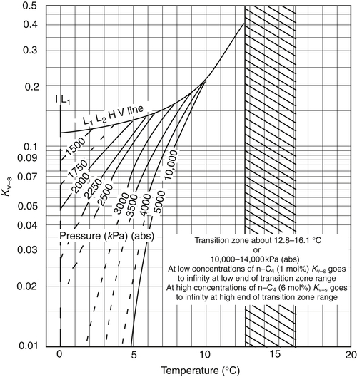
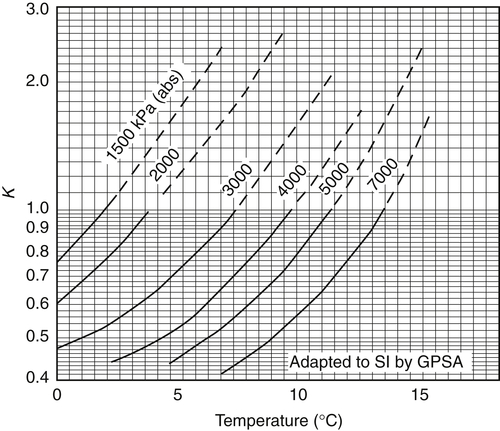
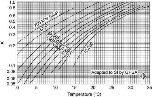
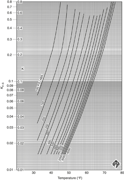
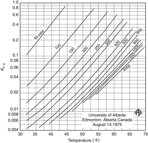
3.2. The K-Factor Method

The second method that lends itself to hand calculations is the K-factor method. This method originated with Carson and Katz (1942) (also see Wilcox et al., 1941), although there have been additional data and charts reported since then. One of the ironies of this method is that the original charts of Carson and Katz (1942) have been reproduced over the years even though they were originally marked as “tentative” by the authors.

The K-factor is defined as the distribution of the component between the hydrate and the gas:

$K_{i} = \frac{y_{i}}{s_{i}}$ $K_{i} = \frac{y_{i}}{s_{i}}$

(3.4)

where y_i and s_i are the mole fractions of component i in the vapor and hydrate, respectively. These mole fractions are on a water-free basis and water is not included in the calculations. It is assumed that sufficient water is present to form a hydrate.

There is a chart available for each of the components commonly encountered in natural gas that is a hydrate former: methane, ethane, propane, isobutane, n-butane, hydrogen sulfide, and carbon dioxide. Versions of these charts, one set in SI units and another in American engineering units, are appended to this chapter.

All nonformers are simply assigned a value of infinity, because, by definition, s_i = 0 for nonformers, there is no nonformer in the hydrate phase. This is true for both light nonformers, such as hydrogen, and heavy ones, such as n-pentane and n-hexane.

At first glance, this seems a little awkward, but it comes out almost naturally when performing the calculations.

3.2.1. Calculation Algorithms

The K-charts are usually used in three methods: (1) given the temperature and pressure calculate the composition of the coexisting phases, (2) given the temperature calculate the pressure at which the hydrate forms and the composition of the hydrate, and (3) given the pressure calculate the temperature at which the hydrate forms and the composition of the hydrate.

3.2.1.1. Flash

The first type of calculation is a flash. In this type of calculation, the objective is to calculate the amount of the phases present in an equilibrium mixture and to determine the composition of the coexisting phases. The temperature, pressure, and compositions are the input parameters.

The objective function to be solved, in the Rachford–Rice form, is:

$f (V) = \sum \frac{z_{i} (1 - K_{i})}{1 + V (K_{i} - 1)}$ $f (V) = \sum \frac{z_{i} (1 - K_{i})}{1 + V (K_{i} - 1)}$

(3.5)

where z_i is the composition of the feed on a water-free basis. An iterative procedure is used to solve the vapor phase fraction, V, such that the function equals zero. This equation is applicable to all components, but may cause numerical problems. The following equation helps to alleviate such problems:

$f (V) = \sum_{former} \frac{z_{i} (1 - K_{i})}{1 + V (K_{i} - 1)} + \sum_{nonformer} \frac{z_{i}}{V}$ $f (V) = \sum_{former} \frac{z_{i} (1 - K_{i})}{1 + V (K_{i} - 1)} + \sum_{nonformer} \frac{z_{i}}{V}$

(3.6)

Once you have calculated the phase fraction, the vapor phase compositions can be calculated as follows:

$y_{i} = \frac{z_{i} K_{i}}{1 + V (K_{i} - 1)}$ $y_{i} = \frac{z_{i} K_{i}}{1 + V (K_{i} - 1)}$

(3.7)

for formers and

$y_{i} = \frac{z_{i}}{V}$ $y_{i} = \frac{z_{i}}{V}$

(3.8)

for nonformers. From the vapor phase, the composition of the solid is calculated from:

$s_{i} = \frac{y_{i}}{K_{i}}$ $s_{i} = \frac{y_{i}}{K_{i}}$

(3.9)

This may be a little difficult to understand, but the s_i is not really meant to be the composition of the hydrate phase. These are merely an intermediate value in the process of calculating the hydrate pressure as a function of the temperature. The objective is to calculate the hydrate locus and not to estimate the hydrate composition.

Only rarely would this type of calculation be used. The calculations in the next section are much more common.

3.2.1.2. Incipient Solid Formation

The other two methods are incipient solid formation points and are equivalent to a dew point. This is the standard hydrate calculation. The purpose of this calculation it to answer the question “Given the temperature and the composition of the gas, at what pressure will a hydrate form?” A similar calculation is to estimate the temperature at which a hydrate will form given the pressure and the composition. The execution of these calculations is very similar.

The objective functions to be solved are:

$f_{1} (T) = 1 - \sum y_{i} / K_{i}$ $f_{1} (T) = 1 - \sum y_{i} / K_{i}$

(3.10)

$f_{2} (P) = 1 - \sum y_{i} / K_{i}$ $f_{2} (P) = 1 - \sum y_{i} / K_{i}$

(3.11)

Depending upon whether you want to calculate the pressure or the temperature, the appropriate function, either Eqn (3.6) or (3.7) is selected. Iterations are performed on the unknown variable until the summation is equal to unity. So to use the first equation (Eqn (3.6)), the pressure is known and iterations are performed on the temperature.

Figure 3.7 shows a simplified pseudo code description of the algorithm for performing a hydrate formation pressure calculation using the K-factor method.

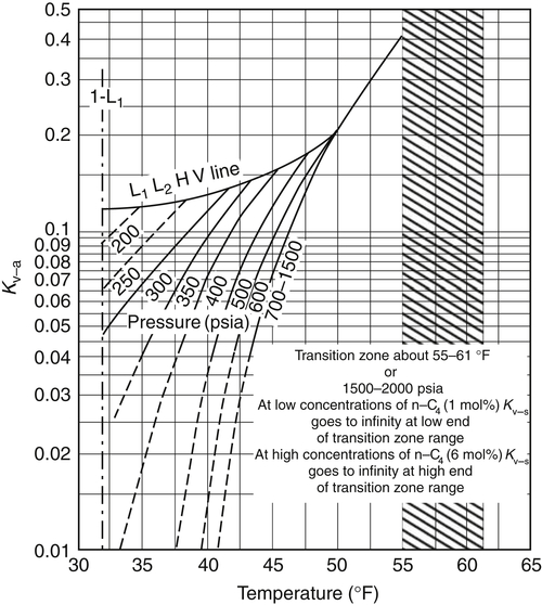
3.2.2. Liquid Hydrocarbons

The K-factor method is designed for calculations involving a gas and a hydrate. In order to extend this method to liquid hydrocarbons, the vapor–liquid K-factor should be incorporated. For the purposes of this book, these K-factors will be denoted K_V in order to distinguish them from the K-factor defined earlier. Therefore, we present the following:

$K_{Vi} = \frac{y_{i}}{x_{i}}$ $K_{Vi} = \frac{y_{i}}{x_{i}}$

(3.12)

where x_i is the mole fraction of component i in the nonaqueous liquid.

If the equilibria involve a gas, a nonaqueous liquid and a hydrate, then the following equations should be solved to find the phase fractions, L and V:

$f_{1} (V, L) = \sum \frac{z_{i} (1 - K_{Vi})}{L (1 - V) + (1 - V) (1 - L) (K_{Vi} / K_{i}) + V K_{Vi}}$ $f_{1} (V, L) = \sum \frac{z_{i} (1 - K_{Vi})}{L (1 - V) + (1 - V) (1 - L) (K_{Vi} / K_{i}) + V K_{Vi}}$

(3.13)

$f_{2} (V, L) = \sum \frac{z_{i} (1 - K_{Vi} / K_{i})}{L (1 - V) + (1 - V) (1 - L) (K_{Vi} / K_{i}) + V K_{Vi}}$ $f_{2} (V, L) = \sum \frac{z_{i} (1 - K_{Vi} / K_{i})}{L (1 - V) + (1 - V) (1 - L) (K_{Vi} / K_{i}) + V K_{Vi}}$

(3.14)

This is a nontrivial problem that requires the solution of two nonlinear equations in two unknowns, L and V, the phase fractions of the liquid and vapor.

Figure 3.7 Pseudo Code for Performing a Hydrate Pressure Estimate Using the Katz K-factor Method.

On the other hand, for equilibria involving a hydrate and a nonaqueous liquid, the K-factors are as follows:

$K_{Li} = \frac{K_{Vi}}{K_{i}} = \frac{s_{i}}{x_{i}}$ $K_{Li} = \frac{K_{Vi}}{K_{i}} = \frac{s_{i}}{x_{i}}$

(3.15)

To determine the incipient solid formation point, the following function must be satisfied:

$\sum \frac{K_{Vi} x_{i}}{K_{i}} = 1$ $\sum \frac{K_{Vi} x_{i}}{K_{i}} = 1$

(3.16)

and, as with the vapor–solid calculation, you can either iterate on the temperature for a given pressure or iterate on the pressure for a given temperature.

The vapor–liquid K-factors can be obtained from the K-factor charts in the GPSA Engineering Data Book or one of the other simple or complex methods available in the literature.

Typically, the problem of calculating the hydrate formation conditions in the presence of liquid hydrocarbon is too difficult for hand calculations. In such cases, it is wise to use one of the commercially available software packages.

3.2.3. Computerization

Ironically, although we have classified these as “hand” calculation methods, the charts have been converted to correlations in temperature and pressure. Sloan (1998) presents a series of correlations based on the charts that are suitable for computer calculations. The correlations are quite complex and will not be repeated here. Because of their complexity, these correlations are not suitable for hand calculations.

The accompanying Web site contains several versions of the K-factor method for computers. They are a series of stand-alone disk operating system programs for performing various calculations, including a hydrate locus prediction. There is one set that uses SI units and the other uses American engineering units.

3.2.4. Comments on the Accuracy of the K-Factor Method

Until about 1975, the K-factor method represented the state of the art for estimating hydrate formation conditions. This method was only supplanted by the more rigorous methods, which are discussed in the next chapter, with the emergence of inexpensive computing power.

The K-factor method, as given on the accompanying Web site, is surprisingly accurate for predicting the hydrate locus of pure methane, ethane, carbon dioxide, and hydrogen sulfide. Figure 3.8 shows a comparison between the hydrate locus based on a correlation of the experimental data (the same as shown in Figure 2.3) and the prediction from the K-factor method for methane and ethane. Figure 3.9 is a similar plot for hydrogen sulfide and carbon dioxide.

These calculations are performed in spite of the warning in the GPSA Engineering Data Book (1998) that these methods should not be used for pure components. It is demonstrated here that the method is surprisingly accurate for methane, ethane, hydrogen sulfide, and carbon dioxide. Although not shown, the method does not work for pure propane, isobutane, and n-butane.

Figure 3.8 Hydrate Loci for Methane and Ethane. (points from correlation, curves from K-factor.)

The K-factor method is poor at low pressure and, thus, it does not predict the hydrate loci for either propane or isobutane in the pure state.

In addition, in order to get a prediction for hydrogen sulfide, the temperature must be at least 10 °C (50 °F), which corresponds to 0.3 MPa (45 psia). Similarly, for ethane, the temperature must be 1.7 °C (35 °F), which is a hydrate pressure of 0.62 MPa (90 psia). In general, it is recommended that the minimum pressure for the use of the correlation is 0.7 MPa (100 psia).

Although the K-factor method works quite well for pure hydrogen sulfide, it should be used with caution (and probably not at all) for sour gas mixtures. H₂S forms a hydrate quite readily and it exerts a large influence on the hydrate forming of mixtures that contains it as a component.

Figure 3.9 Hydrate Loci for Hydrogen Sulfide and Carbon Dioxide. (Points from correlation, curves from K-factor.)

In addition, the method cannot predict the hydrate for liquids (as noted in the text). At the experimental quadruple point, the K-factor method tends to continue to extrapolate as if the fluid were a vapor.

On the other hand, the method is not good for high pressure. For pure methane, the K-factor method does not give results at pressures greater than about 20 MPa (3000 psia), which is about 18 °C (64.5 °F). Fortunately, this range of pressure and temperature is sufficient for most applications. Having said that, it is probably wise to limit the application of this method to pressures less than 7 MPa (1000 psia).

In summary, the recommended ranges for the application of the K-factor method are:

0 < t < 20 °C	32 < t < 68 °F
0.7 < P < 7 MPa	100 < P < 1000 psia

It is probably safe to extrapolate this pressure and temperature range to mixtures. However, the method tends to be less accurate for mixtures.

3.2.4.1. Ethylene

In his studies of hydrate formation in methane-ethylene mixture, Otto (1959) attempted to generate a K-factor chart for ethylene. Although he successfully generated a chart, it was not very successful for predicting the hydrate conditions in ethylene mixtures. Errors as large as 1000–1500 kPa (150–220 psia) were observed when predicting the hydrate pressures for mixtures containing ethylene.

It was demonstrated in Chapter 2 that among hydrate formers, ethylene is unique. This further demonstrates the unusual nature of this component.

3.2.5. Mann et al

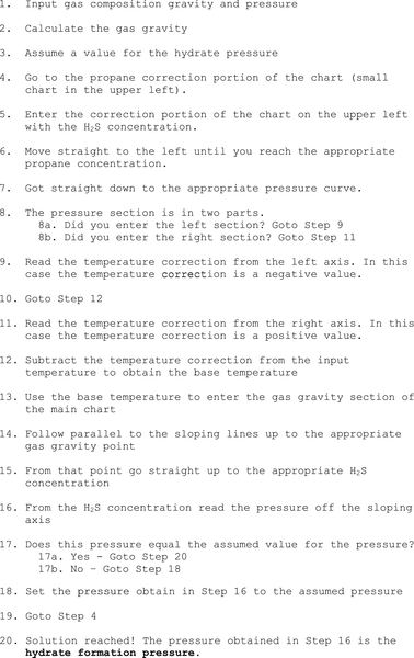
It is possible to include the hydrate type in the K-factor method. For example, Mann et al. (1989) presented two sets of K-factors for the hydrate formers, one for each crystal structure. However, this method has not gained acceptance in the gas processing industry.

The Hydrate + software package from FlowPhase incorporated the Mann et al. method as one of its optional calculation packages.

3.3. Baillie–Wichert Method

Another chart method for hydrate prediction was developed by Baillie and Wichert (1987). The basis for this chart is the gas gravity, but the chart is significantly more complex than the Katz gravity method. The chart is for gases with gravity between 0.6 and 1.0.

In addition to the gravity, this method accounts for the presence of hydrogen sulfide (up to 50 mol%) and propane (up to 10%). The effect of propane comes in the form of a temperature correction, which is a function of the pressure and the H₂S concentration.

Of the simple methods presented in this chapter, only the Baillie–Wichert method is designed for use with sour gas. This is a significant advantage over both the gas gravity and K-factor methods.

Figure 3.10 shows the chart for this method in SI units and Fig. 3.11 is in American engineering units.

The chart was designed to predict the hydrate temperature of a sour gas of known composition at a given pressure. The H₂S content of the sour gas for the application of the chart can be from 1% to 50%, with the H₂S to CO₂ ratio between 10:1 and 1:3. Under these conditions, the chart method usually predicts a hydrate temperature of ±2 °F for 75% of the cases (Wichert, 2004). Baillie and Wichert (1987) state that, for a given pressure, their chart estimates the hydrate temperature to within 1.7 °C (3 °F) for 90% of their tests.

Figure 3.10 Baillie–Wichert Chart for Estimating Hydrate Formation Conditions in SI Units. Reprinted from the GPSA Engineering Data Book, 11th ed.—reproduced with permission.

Furthermore, from the chart itself, it can be seen that the pressure is limited to 4000 psia (27.5 MPa), the gas gravity must be between 0.6 and 1.0, and the propane composition must be less than 10 mol%.

In a study of the hydrate formation in sour gas mixtures, and bearing in mind the limit on the ratio of H₂S to CO₂ given above, Carroll (2004) found that the Baillie–Wichert method has an average error of 2.0 °F (1.1 °C). This method predicts the experimental hydrate temperature to within 3 °F about 80% of the time. This compares well with more rigorous methods, which will be discussed in the next chapter.

Figure 3.11 Baillie–Wichert Chart for Estimating Hydrate Formation Conditions in American Engineering Units. Reprinted from the GPSA Engineering Data Book, 11th ed.—reproduced with permission.

The study presented by Carroll (2004) only included data values in the composition ranges stated by Wichert (2004). If the composition is outside the range given, the errors increase significantly. More discussion of the study of Carroll (2004) is presented later in this chapter.

The use of these charts is neither simple nor intuitive. Figure 3.12 gives the pseudo code for the procedure for estimating the hydrate temperature. This procedure is a once through method resulting directly in the hydrate temperature. Figure 3.13 gives the pseudo code for estimating the hydrate pressure. To use the Baillie–Wichert method to estimate the hydrate pressure requires an iterative procedure. You must start with an estimate of the pressure and iterate until you reach a solution. You can use the Katz gas gravity method to obtain a value for the starting pressure. From this starting point, the method converges in only a few iterations.

Figure 3.12 Pseudo Code for Estimating Hydrate Pressure Using the Baillie–Wichert Method.

Figure 3.13 Pseudo Code for Estimating Hydrate Temperature Using the Baillie–Wichert Method.

3.4. Other Correlations

Although the gas gravity method is not highly accurate, it has a high level of appearance because of its simplicity. Therefore, many authors have attempted to build correlations to describe the relation between the gas gravity and the hydrate pressure. Some of these are described in this section.

These correlations are useful for spreadsheet calculations in addition to hand calculations, but the user is advised to be cautious. These correlations are no more accurate than the original charts. In addition, they are not applicable to sour gas mixtures.

When using these equations, the reader is cautioned to be careful regarding common logarithms (log), which are base 10, and natural logarithms (ln), which are base e.

3.4.1. Makogon

Makogon (1981) provided a simple correlation for the hydrate formation pressure as a function of temperature and gas gravity for paraffin hydrocarbons. His correlation is:

$\log P = β + 0.0497 (t + k t^{2}) - 1$ $\log P = β + 0.0497 (t + k t^{2}) - 1$

(3.17)

where P is in MPa and t is in Celsius. Makogon provided graphic correlations for β and k, but Elgibaly and Elkamel (1998) give the following simple correlations:

$β = 2.681 - 3.811 γ + 1.679 γ^{2}$ $β = 2.681 - 3.811 γ + 1.679 γ^{2}$

(3.18)

$k = - 0.006 + 0.011 γ + 0.011 γ^{2}$ $k = - 0.006 + 0.011 γ + 0.011 γ^{2}$

(3.19)

Note the complete formulation of this correlation, as given in Elgibaly and Elkamel (1998), has errors but their correlation of β and k are correct.

3.4.2. Kobayashi et al

Kobayashi et al. (1987) proposed the following, rather complicated, equation for estimating hydrate formation conditions as a function of the gas gravity:

$\begin{matrix} \frac{1}{T} = 2.7707715 \times 10^{- 3} - 2.782238 \times 10^{- 3} \ln P - 5.649288 \times 10^{- 4} \ln γ \\ - 1.298593 \times 10^{- 3} \ln P^{2} + 1.407119 \times 10^{- 3} \ln (P) \ln (γ) + 1.785744 \times 10^{- 4} \ln {(γ)}^{2} \\ + 1.130284 \times 10^{- 3} \ln {(P)}^{3} + 5.9728235 \times 10^{- 4} \ln {(P)}^{2} \ln (γ) \\ - 2.3279181 \times 10^{- 4} \ln (P) \ln {(γ)}^{2} - 2.6840758 \times 10^{- 5} \ln {(γ)}^{3} \\ + 4.6610555 \times 10^{- 3} \ln {(P)}^{4} + 5.5542412 \times 10^{- 4} \ln {(P)}^{3} \ln (γ) \\ - 1.4727765 \times 10^{- 5} \ln {(P)}^{2} \ln {(γ)}^{2} + 1.393808 \times 10^{- 5} \ln (P) \ln {(γ)}^{3} \\ + 1.4885010 \times 10^{- 5} \ln {(γ)}^{4} \end{matrix}$ $\begin{matrix} \frac{1}{T} = 2.7707715 \times 10^{- 3} - 2.782238 \times 10^{- 3} \ln P - 5.649288 \times 10^{- 4} \ln γ \\ - 1.298593 \times 10^{- 3} \ln P^{2} + 1.407119 \times 10^{- 3} \ln (P) \ln (γ) + 1.785744 \times 10^{- 4} \ln {(γ)}^{2} \\ + 1.130284 \times 10^{- 3} \ln {(P)}^{3} + 5.9728235 \times 10^{- 4} \ln {(P)}^{2} \ln (γ) \\ - 2.3279181 \times 10^{- 4} \ln (P) \ln {(γ)}^{2} - 2.6840758 \times 10^{- 5} \ln {(γ)}^{3} \\ + 4.6610555 \times 10^{- 3} \ln {(P)}^{4} + 5.5542412 \times 10^{- 4} \ln {(P)}^{3} \ln (γ) \\ - 1.4727765 \times 10^{- 5} \ln {(P)}^{2} \ln {(γ)}^{2} + 1.393808 \times 10^{- 5} \ln (P) \ln {(γ)}^{3} \\ + 1.4885010 \times 10^{- 5} \ln {(γ)}^{4} \end{matrix}$

(3.20)

With this set of coefficients, the temperature, T, is in Rankine, the pressure, P, is in psia, and γ is the gas gravity, dimensionless.

Unfortunately, there appears to be something wrong with this equation or with the coefficients given. No matter what value is entered for the pressure, the resulting temperature is always approximately 0 R (−460 °F) (see the example section of this chapter). Much effort was expended trying to find the error (including using natural instead of common logarithms), but the problem could not be completely isolated.

3.4.3. Motiee

Motiee (1991) presented the following correlation for the hydrate temperature as a function of the pressure and the gas gravity:

$T = - 283.24469 + 78.99667 \log (P) - 5.352544 \log {(P)}^{2} + 349.473877 γ - 150.854675 γ^{2} - 27.604065 \log (P) γ$ $T = - 283.24469 + 78.99667 \log (P) - 5.352544 \log {(P)}^{2} + 349.473877 γ - 150.854675 γ^{2} - 27.604065 \log (P) γ$

(3.21)

where T is the hydrate temperature in K, P is the pressure in kPa, and γ is the gas gravity.

3.4.4. Østergaard et al

Another correlation was proposed by Østergaard et al. (2000). These authors began with a relatively simple function of the hydrate formation conditions using the gas gravity method, which is applicable to sweet gas.

Table 3.1

Parameters for the Østergaard et al. Correlation for Hydrate Formation

c₁	4.5134 × 10⁻³	c₆	3.6625 × 10⁻⁴
c₂	0.46852	c₇	−0.485054
c₃	2.18636 × 10⁻²	c₈	−5.44376
c₄	−8.417 × 10⁻⁴	c₉	3.89 × 10⁻³
c₅	0.129622	c₁₀	−29.9351

$\ln (P) = (c_{1} {(γ + c_{2})}^{- 3} + c_{3} F_{m} + c_{4} F_{m}^{2} + c_{5}) T + c_{6} {(γ + c_{7})}^{- 3} + c_{8} F_{m} + c_{9} F_{m}^{2} + c_{10}$ $\ln (P) = (c_{1} {(γ + c_{2})}^{- 3} + c_{3} F_{m} + c_{4} F_{m}^{2} + c_{5}) T + c_{6} {(γ + c_{7})}^{- 3} + c_{8} F_{m} + c_{9} F_{m}^{2} + c_{10}$

(3.22)

where P is the pressure in kPa, γ is the gas gravity, T is the temperature in K, and F_m is the mole ratio between nonformers and formers in the mixture. The constants for this equation are given in Table 3.1.

They then provide a correction for nitrogen and carbon dioxide. Those interested in these corrections should consult with the original paper. In addition, this method is not applicable to pure methane or to pure ethane, both of these gases have gravities outside the range of their correlation.

It is interesting to note that Østergaard et al. (2000) state that they attempted to include H₂S in their correlation, but they were not successful.

A spreadsheet is available from Østergaard et al. to perform calculations using their correlation.

3.4.5. Towler and Mokhatab

Towler and Mokhatab (2005) proposed a relatively simple equation for estimating hydrate temperatures as a function of the pressure and the gas gravity:

$T = 13.47 \ln (P) + 34.27 \ln (γ) - 1.675 \ln (P) \ln (γ) - 20.35$ $T = 13.47 \ln (P) + 34.27 \ln (γ) - 1.675 \ln (P) \ln (γ) - 20.35$

(3.23)

Note that in their original paper, they use log, but it is clear when you use this equation that these are natural logarithms.

3.5. Comments on All of These Methods

In spite of their relative simplicity, these methods are surprisingly accurate. For sweet natural gas mixtures, the gas gravity method is accurate to within 20% or better for estimating hydrate pressures. However, as will be demonstrated, larger errors can be encountered.

The K-factor charts are probably accurate to about 10–15% for similar mixtures. Another inaccuracy is the user's ability to read the chart—they are frustratingly difficult to read! This can also contribute significantly to the error.

The Baillie–Wichert method is better than the gas gravity method when applied to sweet gas. The reason for this is the inclusion of a correction factor for propane. The real advantage of this method is that it is applicable to sour gas mixtures. Of the three methods presented in this chapter, the Baillie–Wichert chart is the method of choice for sour gas mixtures.

However, the question arises “How can these methods be even approximately correct when they do not account for the two different types of hydrates?” The short answer is that they cannot. It is thermodynamically inconsistent for the models not distinguish between the two types.

The long answer to this question is that, for natural gas mixtures, the type II hydrate predominates. Whenever there is only a small amount of type II former present, the resultant hydrate is type II. This change from type I to type II can have a significant effect on the hydrate-forming pressure. For example, pure methane forms a type I hydrate at 15 °C and 12.8 MPa (see Table 2.2). The presence of only 1% propane, a type II former, results in a mixture that forms a type II hydrate. This mixture is estimated to form a hydrate at 15 °C and 7.7 MPa. The mixture calculation is performed using CSMHYD.¹ CSMHYD is one of the computer programs discussed in the next chapter.

Before the widespread use of computers and the availability of software (pre-1970s), the K-factor method of Katz and co-workers was the state of the art, and it remains very popular in spite of its drawbacks.

Doing calculations when liquid hydrocarbons are present are very difficult via methods designed for hand calculations, and the results are usually not highly accurate. Therefore, it is usually not worth the time to do these types of calculations by hand.

3.5.1. Water

All of the chart methods assume that there is plenty of water present in the system. Thus, these methods predict the worst-case for the hydrate-forming conditions. These methods should not be used to estimate the hydrate-forming conditions in a dehydrated gas.

3.5.2. Nonformers

It is interesting to contrast the effect of nonformers on the predicted formation conditions from these methods.

A light nonformer, such as hydrogen, will reduce the gravity of the gas. In the gas gravity method, the presence of such a gas decreases the gravity of the gas and, thus, it is predicted to increase the pressure at which a hydrate will form for a given temperature. On the other hand, the presence of a heavy nonformer, such as n-pentane, would increase the gravity of the gas and, thus, it is predicted to decrease the hydrate pressure. The gravity effect of the nonformers is approximately the same for the Baillie–Wichert method, except for the two components for which there are correction factors.

On the other hand, the K-factor method handles all nonformers the same way. All nonformers are assigned a K-factor of infinity. Therefore, the presence of any nonformer, be it heavy or light, is predicted to increase the pressure at which a hydrate will form for a given temperature.

Note there is a contrast for the prediction of the effect of a heavy nonformer on the hydrate pressure. The gas gravity method predicts that the heavy component will decrease the hydrate pressure, whereas the K-factor method predicts an increase in the pressure. What do the experimental data say?

Ng and Robinson (1976) measured the hydrate locus for a mixture of methane (98.64 mol%) and n-pentane (1.36%). They found that the locus for the mixture was at higher pressure than the locus for pure methane. This is consistent with the K-factor approach and is contrary to the behavior predicted by the gas gravity method.

On the other hand, both the gas gravity and K-factor methods predict that a light nonformer would increase the hydrate pressure. Again, it is interesting to examine the experimental evidence.

Zhang et al. (2000) measured the hydrate-forming conditions for several hydrocarbon + hydrogen mixtures. In every case, the presence of hydrogen increased the hydrate formation pressure. This is consistent with the predictions from both the gas gravity and K-factor methods.

One word of caution about this simplified discussion. The addition of a heavy nonformer may lead to the formation of a hydrocarbon liquid phase. The effect of the formation of this phase should not be overlooked.

3.5.3. Isobutane vs n-Butane

As was discussed in Chapter 2, isobutane is a true hydrate former inasmuch as it will form a hydrate without other hydrate formers present. On the other hand, n-butane will only enter the hydrate lattice in the presence of another hydrate former. In some sense, both of these components are hydrate formers and, therefore, it is interesting to compare how these simple methods for estimating hydrate formation handle these two components.

In both the gas gravity and Baillie–Wichert methods, it does not matter whether the butane is in the iso form, the normal form, or a mixture of the two. A mixture containing 1 mol% isobutane will have the same molar mass as a mixture containing 1 mol% n-butane. Because the molar masses are the same, then the gas gravities are the same. Also, because the gas gravities are the same, then the predicted hydrate formation conditions are the same for these two mixtures. The same is true for the Baillie–Wichert method. Their method distinguishes propane, but does not include the effect of the butanes, except through their effect on the gravity.

On the other hand, the K-factor method treats these components as separate and distinct components. There are separate charts for the K-factors of isobutane and n-butane, and from these charts one obtains unique K-factors for these two components.

Consider the simple example of two gas mixtures: (1) 96.8 mol% methane and 3.2% isobutane and (2) 96.8 mol% methane and 3.2% n-butane. Both of these mixtures have a gravity of 0.600.

From the gas gravity method, both of these mixtures would have the same hydrate formation conditions. For example, at 2 MPa, the hydrate temperature is estimated to be about 5.7 °C. The Baillie–Wichert method does not distinguish between these two mixtures either. Using their chart, the hydrate temperature is also estimated to be about 5.7 °C.

On the other hand, the K-factor method produces significantly different results. Using the programs on the accompanying Web site, the hydrate temperature for the first mixture is estimated to be 10.6 °C and 2.1 °C for the second mixture.

The reader should attempt to reproduce these calculations for themselves and, therefore, to verify these observations.

It is a little difficult at this point to answer the question “Which one is correct?” However, in a subsequent section of this chapter, the accuracy of the K-factor method for mixtures of methane and n-butane is discussed. At this point, it is sufficient to say that the K-factor method predicts the experimental data for these mixtures to better than 2 °C.

In the next chapter, we will examine some more advanced methods for calculating hydrate formation, including some commercial software packages. One of these software packages is EQUI-PHASE Hydrate.² This program estimates that the hydrate temperature for the first mixture is 9.6 °C and for the second mixture it is 1.3 °C, which are in reasonable agreement with the K-factor method. Therefore, it is fair to conclude that the K-factor better reflects the actual behavior than those methods based on gas gravity.

3.5.4. Quick Comparison

The next several examples will be compared with the predictions largely from the K-factor method. The mixtures examined are as follows: (1) a synthetic natural gas consisting only of light hydrocarbons, (2) two mixtures rich in carbon dioxide, and (3) mixtures of methane and n-butane.

3.5.4.1. Mei et al. (1998)

Mei et al. (1998) obtained the hydrate locus for a synthetic natural gas mixture. The mixture is largely methane (97.25 mol%), but includes ethane (1.42%), propane (1.08%), and isobutane (0.25%). This gas has a gravity of 0.575. These data are so new that they could not have been used in the development of the models and thus provide a good test of said models.

Figure 3.14 shows the experimental data from Mei et al. (1998), the locus for pure methane (from Chapter 2), and the predicted hydrate locus from the gas gravity and K-factor methods.

The K-factor method is surprisingly good. For a given pressure, the K-factor method predicts the hydrate temperature to within 1 °C; or looking at it from the other direction, for a given temperature the method predicts the pressure to within 10%.

On the other hand, the gravity method exhibits a significant error. For a given temperature, the gravity method predicts a hydrate pressure that is approximately double the measured value. This is a simple yet realistic composition for a natural gas, and this example clearly demonstrates the potential errors from the simple gas gravity method. It should now be clear that this chart does not represent the definitive map of the hydrate formation regions.

Figure 3.14 Hydrate Locus for a Synthetic Natural Gas Mixture. (SG = 0.575) (CH₄ 97.25 mol%, C₂H₆ 1.42%, C₃H₈ 1.08, i-C₄H₁₀ 0.25%).

The gravity of this mixture is lighter than the minimum used with the Baillie–Wichert chart, so no comparison was made. However, it is worth noting that the Baillie–Wichert method does include a correction for propane.

The hydrate locus for pure methane is included for comparison purposes. It is interesting to note the effect of a seemingly small amount of “other” components can have on the hydrate locus. The experimental mixture contains 97.25% methane, which for many other purposes would be safe to assume that this mixture has the properties of pure methane. Yet, the hydrate for this mixture forms at pressures almost 2/5 that of pure methane. For example, the experimental hydrate pressure for this mixture at 2 °C is about 1200 kPa, whereas for pure methane it is about 3100 kPa—a ratio of 0.39.

3.5.4.2. Fan and Guo (1999)

Fan and Guo (1999) measured the hydrate loci for two mixtures rich in carbon dioxide. Again, none of these data was used to generate the K-factor charts. These mixtures should prove to be a difficult test because it is commonly believed that the K-factor method is not highly accurate for CO₂-rich fluids.

These mixtures are too rich in CO₂ to expect either the gas gravity or Baillie–Wichert methods to be applicable. In addition, the gravity of these mixtures is much greater than the maximum for use with either the gas gravity or Baillie–Wichert methods, so no comparison is made.

Figure 3.15 shows the hydrate locus for a binary mixture of CO₂ (96.52 mol%) and CH₄ (3.48%). Both the experimental values and the prediction using the K-factor method are plotted.

At low temperature, the K-factor method tends to overpredict the hydrate pressure. On the other hand, at high temperature, the K-factor method tends to underpredict the hydrate pressure. The transition temperature is at about 7 °C (45 °F), although the somewhat sparse nature of the data make the exact point difficult to determine.

Overall, the average absolute error in the estimated hydrate pressure is 0.25 MPa (36 psia).

The second mixture is composed of CO₂ (88.53 mol%), CH₄ (6.83%), C₂H₆ (0.38%), and N₂ (4.26%). Figure 3.16 shows the experimental data and the K-factor prediction for this mixture. Over this range of temperature, the K-factor method is an excellent prediction of the experimental data. The average absolute error is only 0.05 MPa (7 psia).

Figure 3.15 Hydrate Locus for a Mixture of Carbon Dioxide. (96.52 mol%) and methane (3.48 mol%).

Figure 3.16 Hydrate Locus for the Quaternary Mixture. (88.53 mol% CO₂, 6.83% CH₄, 0.38% C₂H₆, 4.26% N₂).

3.5.4.3. Ng and Robinson (1976)

An important study is that of Ng and Robinson (1976). This study was discussed earlier because of its importance in determining the true role of n-butane in the formation of hydrates. Contrary to the other experimental data examined here, it is likely that these data were used to develop the K-factor chart for n-butane. However, they are an interesting set of data nonetheless.

They measured the hydrate loci for four binary mixtures of methane and n-butane. Three of these hydrate loci are shown in Fig. 3.17. The fourth locus was omitted for clarity.

It is clear from these plots that something unusual occurs with the K-factor prediction at about 11 °C (52 °F). The curve for the mixture leanest in n-butane has a noticeable hump at approximately this temperature. The two mixtures richest in n-butane show a more dramatic transition.

Figure 3.17 Hydrate Loci for Three Mixtures of Methane and n-Butane.

Furthermore, above 11 °C, there is an inversion in the predicted behavior. At low temperature, the hydrate pressure decreases with increasing n-butane content. This is the behavior observed from the experimental data, regardless of the temperature. The prediction inverts for temperatures greater than 11 °C. For high temperatures, the hydrate pressure increases with increasing n-butane content.

The reason for this strange prediction can at least be partially explained by examining the K-factor plot for n-butane. At this temperature, all of the isobars converge to a single curve that extends to a higher temperature.

3.5.5. Sour Natural Gas

Carroll (2004) performed a study to determine the accuracy of hydrate prediction methods for sour gas mixtures. A database of experimental points was obtained from the literature. It included measurements from three different laboratories and a total of 125 points. The temperatures ranged from approximately 3 to 27 °C (37°–80 °F). All of the mixtures contained some hydrogen sulfide (and hence were sour) and a few also contained carbon dioxide.

Carroll (2004) found that the K-factor method performed poorly. The simple K-factor method, also designed for hand calculations, had an average error of 2.7 °F (1.5 °C). The method predicted the experimental hydrate temperature to within 3 °F 60% of the time.

On the other hand, the modified K-factor method of Mann et al. (1989) was as accurate as the more rigorous computer models. The average error for the method of Mann et al. (1989) was 1.5 °F (0.8 °C) and it predicted the hydrate temperature to within 3 °F (1.7 °C) about 90% of the time. These errors are comparable to those from the more rigorous models presented in the next chapter.

The study of Carroll (2004) also included predictions from the Baillie–Wichert chart. These results are discussed in the section on the Baillie–Wichert method.

3.6. Local Models

There are several rigorous models for calculating hydrate conditions; many will be discussed in the next chapter. Local models are simplified models used over a small range of temperature and pressure. They are used when the calculation device has limited computing and data storage capabilities, such as a control device (a programmed logic controller) or a spreadsheet, or perhaps, in a worst-case scenario, a hand-held calculator. We can use some of the information provided in this chapter and the preceding chapter to develop these models.

For a fixed composition, the general form of the function for the hydrate locus is:

$P_{hyd} = f (T, x)$ $P_{hyd} = f (T, x)$

(3.24)

There is some theoretical basis to an equation of the form:

$\ln P_{hyd} = a + b / T$ $\ln P_{hyd} = a + b / T$

(3.25)

which is similar to the Clapeyron correlation for vapor pressures. The temperature range (and hence the pressure range) depends upon the system under consideration. The model developer should verify the applicability of such an equation for their given application. As will be shown, failure to do so can lead to significant errors.

In addition, this approach works quite well for a fixed composition. Adjusting it for variable composition is discussed in a subsequent section of this paper.

Assuming that a is a linear function of the temperature gives the following equation:

$\ln P_{hyd} = a + \frac{b}{T} + c T$ $\ln P_{hyd} = a + \frac{b}{T} + c T$

(3.26)

Assuming that a is a constant and b is a function of the temperature results in an equation with a form exactly the same as Eqn (3.24).

$\ln P_{hyd} = a + \frac{b}{T + c}$ $\ln P_{hyd} = a + \frac{b}{T + c}$

(3.27)

In the natural gas business, it is common to require the hydrate formation temperature given the pressure. Thus, Eqn (3.25) can be rearranged to obtain:

$T_{hyd} = \frac{b}{\ln P - a}$ $T_{hyd} = \frac{b}{\ln P - a}$

(3.28)

In the selection of a local model, it is convenient for the equation to be explicit in both temperature and pressure. It would be inconvenient to have a model that required an iterative solution. Thus, an equation like Eqn (3.28) is useful for calculating hydrate pressure; it cannot be rearranged to get a form explicit in the temperature.

Equation (3.28) could be rearranged into a quadratic, but this is still too complex for our purposes. The solution to such an equation is too cumbersome.

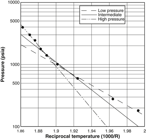
3.6.1. Wilcox et al. (1941)

Consider the hydrate data taken by Wilcox et al. (1941) for what they labelled gas B. This is a relatively light, sweet gas mixture. In total, there are nine points for this composition ranging in pressure from 182 to about 4000 psia.

If one simply uses statistical software, using Eqn (3.25) to fit the all of the data appears to give a good correlation (r² = 0.98624). The resulting correlation is:

$\ln P_{hyd} = 51.66789 - \frac{23, 42433}{T}$ $\ln P_{hyd} = 51.66789 - \frac{23, 42433}{T}$

(3.29)

where P_hyd is in psia and T is in R. However, a plot of the data shows systematic deviations between the correlation and the experimental data. This is shown in Fig. 3.18. At high and low pressure, the correlation underpredicts the hydrate pressure, whereas at intermediate pressure it overpredicts. The average absolute error (AAE) in the predicted hydrate temperature is 1.8 °F.

Figure 3.18 The Hydrate Data for the Wilcox et al. (1941) Gas B and the Fit of the Data Given by Eqn (3.29).

Next, the data were localized—examined over a narrower range of pressure (and hence temperature). The data were separated into three pressure regions: low (180–1000 psia), intermediate (600–1750 psia), and high (1400–4000 psia). Data from the three regions were then fit to an equation of the form given by Eqn (3.25). The results of the fitting are summarized in Table 3.2 and are shown graphically in Fig. 3.19.

Again, merely looking at the statistical results from the data, fitting may not reveal exactly how good or bad the correlation is. However, from the graph, it is clear that the fit is very good if one only considers the range of pressure used to develop the correlation. Extrapolating the curve results in very large errors. However, this is the definition of a local model.

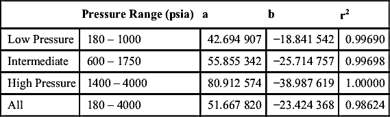
Table 3.2

Summary of Fitting Parameters for the Local Models for the Wilcox et al. (1941) Gas B

	Pressure Range (psia)	a	b	r²
Low Pressure	180 – 1000	42.694 907	−18.841 542	0.99690
Intermediate	600 – 1750	55.855 342	−25.714 757	0.99698
High Pressure	1400 – 4000	80.912 574	−38.987 619	1.00000
All	180 – 4000	51.667 820	−23.424 368	0.98624

Figure 3.19 Local Modelling of the Hydrate Data from Wilcox et al. (1941) for Gas B.

3.6.2. Composition

The common parameter for characterizing the composition of a natural gas mixture is the gas gravity, γ, or equivalently the molecular weight. Therefore, for small variations in the composition, we can propose a local model of the form:

$P_{hyd} = f (T, x, γ)$ $P_{hyd} = f (T, x, γ)$

(3.30)

Based on Eqn (3.25), perhaps we could use something of the form:

$\ln P_{hyd} = a + b γ + \frac{c + d γ}{T}$ $\ln P_{hyd} = a + b γ + \frac{c + d γ}{T}$

(3.31)

Basically, this equation is constructed by assuming that the parameters in Eqn (3.25) are functions of the gas gravity. However, if we are considering a relatively narrow range of temperature (and remember T is the absolute temperature), then this equation becomes:

$\ln P_{hyd} = a + b γ + \frac{c}{T}$ $\ln P_{hyd} = a + b γ + \frac{c}{T}$

(3.32)

Alternatively, we could develop and equation of the form:

$\frac{1000}{T} = a + b P + c \ln P + d γ$ $\frac{1000}{T} = a + b P + c \ln P + d γ$

(3.33)

Other functions could be used for the functional relationship between the temperature, pressure and the composition.

3.6.2.1. Sun et al

Sun et al. (2003) took a set of measurements for sour gas mixtures; remember sour gas being a mixture containing H₂S. These data are from 1 to 26.5 °C and 0.58 to 8.68 MPa. The specific gravity of these mixtures range from 0.656 to 0.787. The data set is approximately 60 points in total. It was noted earlier that the simple gas gravity method is not applicable to sour gas mixtures, thus, this set of data provide a severe test for our simplified local models.

Using least-squares regression to fit the set of data, one obtains the following correlation:

$\frac{1000}{T} = 4.343295 + 1.07340 \times 10^{- 3} P - 9.19840 \times 10^{- 2} \ln P - 1.071989 γ$ $\frac{1000}{T} = 4.343295 + 1.07340 \times 10^{- 3} P - 9.19840 \times 10^{- 2} \ln P - 1.071989 γ$

(3.34)

The average error for this equation is 0.01 °C, the AAE is 1.16 and the maximum error is 2.8 °C. One would expect an average error near zero for this type of correlation and that is what was obtained.

Figure 3.20 Local Modelling for the Sour Gas Data from Sun et al. (2003) Showing the Fit of Eqn (3.34).

Figure 3.20 shows the data of Sun et al. (2003) and the calculation from the local model. The first observation we can make from this set of data is that as the gas gravity increases so does the hydrate temperature.

We will revisit the data of Sun et al. (2003) in the next chapter.

Examples

Example 3.1

Use the gas gravity method to calculate the hydrate formation pressure of ethane at 10 °C. The value in Table 2.3 is about 1.68 MPa.

Answer: The molar mass of ethane is 30.070 and thus:

$γ = 30.070 / 28.966 = 1.038$ $γ = 30.070 / 28.966 = 1.038$

Extrapolating the gravity chart, one reads about 1.25 MPa. This is an error of about 25%, which seems unreasonably large.

Example 3.2

Use the gravity method to calculate the pressure at which a hydrate will form at 14.2 °C for the following mixture:

CH₄	0.820
CO₂	0.126
H₂S	0.054

The experimental value is 4.56 MPa.

Answer: Calculate the molar mass of the gas mixture:

$0.820 \times 16.043 + 0.126 \times 44.011 + 0.054 \times 34.082 = 20.541$ $0.820 \times 16.043 + 0.126 \times 44.011 + 0.054 \times 34.082 = 20.541$

$γ = 20.541 / 28.966 = 0.709$ $γ = 20.541 / 28.966 = 0.709$

From Fig. 3.2, we read slightly less than 4.0 MPa—very good agreement, especially considering that this is a sour gas.

Example 3.3

Repeat the above calculation using the K-factor method.

Answer: As a first guess, assume that the pressure is 4 MPa, selected because of ease of reading the chart. However, the values for CO₂ must be extrapolated at this pressure. A second iteration is performed at 5 MPa.

The iterations are summarized in the table below. The charts are not easily read to a greater accuracy than 1 MPa or so, so there is no point in repeating the iteration beyond this seemingly crude level.

	4 MPa		5 MPa
	K_i	y_i/K_i	K_i	y_i/K_i
CH₄	1.5	0.547	1.35	0.607
CO₂	∼3	0.042	2	0.063
H₂S	0.21	0.257	0.18	0.300
		Sum = 0.846		Sum = 0.970

Linearly extrapolating from the results in the table yields 5.24 MPa. The result is somewhat greater than the experimental value. A significant portion of this error lies in one's ability to read the charts. This includes the need to extrapolate some of the curves.

Example 3.4

Use the correlations from Sloan (1998) to redo Example 3.2. An Excel spreadsheet is available for these calculations; however, it requires engineering units. Converting 14.2 °C gives 57.6 °F.

Answer: Based on the previous calculations, assume a pressure of 700 psi and iterate from there.

700 psi	Sum = 0.925
750 psi	Sum = 0.945
800 psi	Sum = 0.983
825 psi	Sum = 1.001

Therefore, the answer is approximately 825 psi or 5.69 MPa, which represents an error of about 25%.

Clearly, using the correlations of Sloan (1998) and some computing power makes these calculations significantly easier.

Example 3.5

For the mixture given in Example 3.2, calculate the composition of the hydrate at 15 °C and 6.5 MPa. Use the correlations of Sloan (1998) to obtain the K-factors.

Answer: Again, convert to engineering units: 59 °F and 943 psi. At these conditions, the K-factors are:

CH₄	1.228
CO₂	2.289
H₂S	0.181

Iterate on Eqn (3.2) until the sum is zero. The Excel spreadsheet is set up to facilitate this iteration.

V = 0.5	Sum = −0.1915
V = 0.75	Sum = −0.1274
V = 0.9	Sum = −0.0620
V = 0.95	Sum = −0.0274
V = 0.99	Sum = +0.0098 finally spanned the answer!
V = 0.9795	Sum = −0.0011
V = 0.9806	Sum = +0.0000 solution reached!

As an initial starting point, I usually select a phase fraction of 0.5. From there, I iterate toward the answer in a somewhat arbitrary manner. Once I get close to the answer (preferably spanning the answer), I switch to a linear interpolation method. I use the two iterates that span the answer and linearly interpolate for my next estimates.

Therefore, the mixture is 98 mol% gas. The compositions of the two phases, which are also calculated in the spreadsheet, are as follows:

	Feed	Vapor	Solid
CH₄	0.820	0.8230	0.6704
CO₂	0.126	0.1274	0.0556
H₂S	0.054	0.0496	0.2740

Again, it is important to note that all of these compositions are on a water-free basis.

Example 3.6

Estimate the hydrate temperature for the following mixture at 5 MPa using the Baillie–Wichert chart.

Methane	86.25 mol%
Ethane	6.06%
Propane	2.97%
Isobutane	0.31%
n-Butane	0.63%
Pentanes	0.20%
Hexanes	0.02%
CO₂	1.56%
H₂S	2.00%

Answer: First, estimate the molar mass and gravity of the gas. This is done by multiplying the mole fraction of a component times that molar mass of the component and then summing all of these quantities. Therefore:

Methane	0.8625 × 16.043 = 13.887
Ethane	0.0606 × 30.070 = 1.822
Propane	0.0297 × 44.097 = 1.310
Isobutane	0.0031 × 58.125 = 0.180
n-Butane	0.0063 × 58.125 = 0.366
Pentanes	0.0020 × 72.150 = 0.144
Hexanes	0.0002 × 86.177 = 0.017
CO₂	0.0156 × 44.010 = 0.687
H₂S	0.0200 × 34.080 = 0.682
	M = 19.045 g/mol

$γ = M / 28.966 = 19.0145 / 28.966 = 0.6575$ $γ = M / 28.966 = 19.0145 / 28.966 = 0.6575$

Enter the main chart along the sloping axis at 5 MPa and go across to the 2 mol% H₂S curve (the second of the family of curves). From that point, you go straight down until you reach the 0.6575 gravity point. Then you follow the sloping lines down to the temperature axis. This value is the base temperature. In this case, the base temperature is about 16.7 °C.

Now, go to the temperature correction chart in the upper left. Enter the chart at 2 mol% H₂S and move across to the 2.97 mol% propane (essentially 3 mol%). From that point, you go down to the 5 MPa curve. This is on the right side of the chart so you go to the right axis. At that point, you read that the temperature correction is +1.5 °C—a positive value because it comes from the right half of the correction chart.

The hydrate temperature is the sum of these two terms:

$T_{hyd} = 16.7 + 1.5 = 18.2 ° C$ $T_{hyd} = 16.7 + 1.5 = 18.2 ° C$

Example 3.7

Estimate the hydrate formation temperature at 1000 psia for a gas with a 0.6 gravity using the Kobayashi et al. equation. Assume that there is CO₂, H₂S, and N₂ in the gas. From Fig. 3.3, the temperature is 60 °F.

Answer: Substituting 1000 psia and 0.6 gravity onto the Kobayiashi et al. correlation yields:

$\begin{matrix} \frac{1}{T} = 2.7707715 \times 10^{- 3} - 2.782238 \times 10^{- 3} \ln (1000) - 5.649288 \times 10^{- 4} \ln (0.6) \\ - 1.298593 \times 10^{- 3} \ln {(1000)}^{2} + 1.407119 \times 10^{- 3} \ln (1000) \ln (0.6) + 1.785744 \times 10^{- 4} \ln {(0.6)}^{2} \\ + 1.130284 \times 10^{- 3} \ln {(1000)}^{3} + 5.9728235 \times 10^{- 4} \ln {(1000)}^{2} \ln (0.6) \\ - 2.3279181 \times 10^{- 4} \ln (1000) \ln {(0.6)}^{2} - 2.6840758 \times 10^{- 5} \ln {(0.6)}^{3} \\ + 4.6610555 \times 10^{- 3} \ln {(1000)}^{4} + 5.5542412 \times 10^{- 4} \ln {(1000)}^{3} \ln (0.6) \\ - 1.4727765 \times 10^{- 5} \ln {(1000)}^{2} \ln {(0.6)}^{2} + 1.393808 \times 10^{- 5} \ln (1000) \ln {(0.6)}^{3} \\ + 1.4885010 \times 10^{- 6} \ln {(0.6)}^{4} \end{matrix}$ $\begin{matrix} \frac{1}{T} = 2.7707715 \times 10^{- 3} - 2.782238 \times 10^{- 3} \ln (1000) - 5.649288 \times 10^{- 4} \ln (0.6) \\ - 1.298593 \times 10^{- 3} \ln {(1000)}^{2} + 1.407119 \times 10^{- 3} \ln (1000) \ln (0.6) + 1.785744 \times 10^{- 4} \ln {(0.6)}^{2} \\ + 1.130284 \times 10^{- 3} \ln {(1000)}^{3} + 5.9728235 \times 10^{- 4} \ln {(1000)}^{2} \ln (0.6) \\ - 2.3279181 \times 10^{- 4} \ln (1000) \ln {(0.6)}^{2} - 2.6840758 \times 10^{- 5} \ln {(0.6)}^{3} \\ + 4.6610555 \times 10^{- 3} \ln {(1000)}^{4} + 5.5542412 \times 10^{- 4} \ln {(1000)}^{3} \ln (0.6) \\ - 1.4727765 \times 10^{- 5} \ln {(1000)}^{2} \ln {(0.6)}^{2} + 1.393808 \times 10^{- 5} \ln (1000) \ln {(0.6)}^{3} \\ + 1.4885010 \times 10^{- 6} \ln {(0.6)}^{4} \end{matrix}$

If we examine this term-by-term, the following table results:

	Coefficient	C_ij log(P)ⁱ log(γ)^j
C1	2.7707715E-03	2.7707715E-03
C2	−2.7822380E-03	−1.9219019E-02
C3	−5.6492880E-04	2.8858011E-04
C4	−1.2985930E-03	−6.1965070E-02
C5	1.4071190E-03	−4.9652423E-03
C6	1.7857440E-04	4.6597707E-05
C7	1.1302840E-03	3.7256187E-01	←
C8	5.9728235E-04	−1.4558822E-02
C9	−2.3279181E-04	−4.1961402E-04
C10	−2.6840758E-05	3.5777731E-06
C11	4.6610555E-03	1.0612851E+01	←
C12	5.5542412E-04	−9.3520806E-02
C13	−1.4727765E-05	−1.8338174E-04
C14	1.3938080E-05	−1.2833878E-05
C15	1.4885010E-06	1.0135375E-07
		Sum = 1.0793677E+01

Finally, from the sum, one can calculate the temperature: T = 1/10.793677 = 0.0926 R, which is clearly in error. There appears to be two terms that are problematic: the C7 term and, in particular, the C11 term.

Appendix 3A Katz K-Factor Charts

The K-factor charts for performing hydrate calculations are collected in this appendix. There are two charts for each of the components commonly found in natural gas. One chart is in SI units and the other is in American engineering units. These figures are taken from the GPSA Engineering Data Book and are reproduced here with permission (Figs 3.1a–3.14a).