The subject of this chapter is the inhibition of hydrates using chemicals. The main focus of this chapter is the thermodynamic inhibitors: alcohol, glycol, and ionic salts. Methods are presented for estimating the effect of these chemicals. A thorough review of the use of methanol, the most common hydrate inhibitor, is presented. This includes providing the reader with the tools to estimate the required methanol injection rate, including loses to the vapor and the hydrocarbon liquid. Important properties of the inhibitors are also discussed in some detail, including safety aspects. Sections are also included covering the so-called low dosage inhibitors: kinetic inhibitors and anti-agglomerants. Case studies are presented that demonstrate the effectiveness of the low-dose inhibitors.
As has been stated earlier, hydrates are a significant problem in the natural gas industry. So what can be done when we encounter hydrates in our processes? What can we do to prevent them from forming in the first place? This chapter outlines some design information for battling hydrates using chemicals.
People who live in colder climates are well aware of methods for combating ice. In the winter, salt is often used to remove ice from roads and sidewalks. A glycol solution is sprayed on airplanes waiting for take-off in order to de-ice them. Similar techniques are used for combating hydrates.
Polar solvents, such as alcohol, glycol, and ionic salts (common table salt), are known to inhibit the formation of gas hydrates. It is important to note that they do not prevent hydrate formation, they inhibit it. That is, they reduce the temperature or increase the pressure at which a hydrate will form. The mere presence of an inhibitor does not mean that a hydrate will not form. The inhibitor must be present in some minimum concentration to avoid hydrate formation. The calculation of this minimum inhibitor concentration is addressed in detail in this chapter.
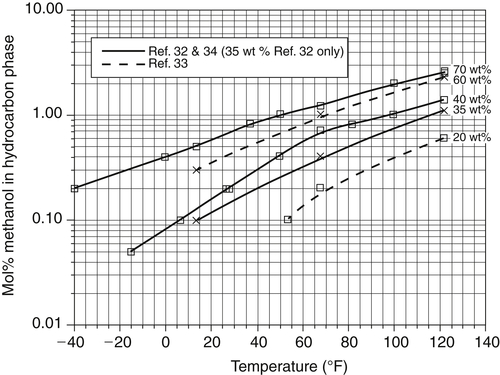
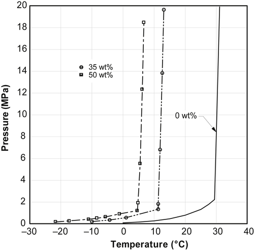
In the natural gas industry, the use of alcohols, particularly methanol, and glycols, EG, or triethylene glycol (TEG), is a common method for inhibiting hydrate formation. Figure 5.1 shows the inhibiting effect of methanol on the hydrate of hydrogen sulfide. The curve for pure H2S is taken from Table 2.6 and the methanol data are from Ng et al. (1985). The curves for the methanol data are merely lines through the data points. They do not represent a prediction or fit of the data. This figure is presented as an example of the inhibiting effect. More such charts for other components will be presented later in this chapter.
Table 5.1 lists the properties of some common polar compounds that are used as inhibitors. Note that all of these compounds exhibit some degree of hydrogen bonding, and thus interfere with water's hydrogen bonds.
Ionic solids, such as sodium chloride (common table salt), also inhibit the formation of hydrates. This is similar to spreading salt on icy sidewalks or highways to melt the ice. It is unlikely that anyone would use salt as an inhibitor; the salt is almost always present in the produced water.
Figure 5.1The Inhibiting Effect of Methanol on the Hydrate of Hydrogen Sulfide.
Although they would never be used as inhibitors per se, the alkanolamines, used for sweetening natural gas, also inhibit the formation of hydrates. The benefit of this is that the risk of hydrate formation in the amine unit is reduced because of the inhibiting effect of the amine.
5.1. Freezing Point Depression
The depression of the freezing point of a solvent by the presence of a small amount of solute is a fairly well-understood concept. In fact, the depression of the freezing point is commonly used to estimate the molar mass of a sample.
The theory behind freezing point depression can be found in any book on physical chemistry (for example, Laidler and Meiser, 1982). The derivation begins with the fundamental relationship for the equilibrium between a solid and a liquid and, after some simplifying assumptions, the resulting equation is:
xi=hslΔTRT2m
(5.1)
where xi is the mole fraction of the solute (inhibitor), ΔT is the temperature depression in °C, R is the universal gas constant (8.314J/molK), and Tm is the melting point of the pure solvent in K. Rearranging this equation slightly and converting from mole fraction to mass fraction gives:
ΔT=MsRT2mhsl×Wi(100−Wi)Mi=KSWi(100−Wi)Mi
(5.2)
where Ms is the molar mass of the solvent, Wi is the weight percent solute (inhibitor), and Mi is the molar mass of the inhibitor. For water, it is KS=1861, when SI units are used. The leading term in this equation contains only constants, so the freezing point depression is a function of the concentration of the inhibitor and its molar mass.
It is worth noting that this equation is not applicable to ionic solutions, such as salt. This will be demonstrated later in this chapter.
To get a quick impression of the accuracy of Eqn (5.2), consider Fig. 5.2, which shows the freezing points of methanol+water and EG+water solutions. The freezing point depression for methanol is quite accurate up to concentrations of 30wt%. For EG, the calculation is accurate only up to about 15wt%. The fit for methanol+water is quite good because the solution is close to ideal. That is because the assumptions built into the derivation are applicable for methanol+water over a fairly wide range of concentration.
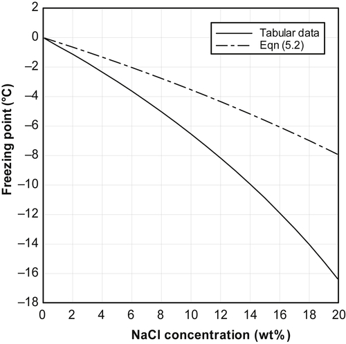
On the other hand, Fig. 5.3 shows the freezing point of sodium chloride (common salt) solutions. From this plot, it is clear that the true freezing points of salt solutions are much lower than those predicted by the simple freezing point depression theory.
Figure 5.2Freezing Points of Methanol+Water and Ethylene Glycol (EG) +Water Mixtures.
Figure 5.3Freezing Points of NaCl (Salt)+Water Mixtures.
In both Figs 5.2 and 5.3, the curves labeled “Tabular Data” are from the CRC Handbook (Weast, 1978).
To use the freezing point depression method to find the molar mass of an unknown substance is relatively simple. It is quite straightforward to make a solution with a known weight fraction even though the nature of the solute is unknown. Adding 5g of solute to 95g of solvent makes a 5wt% solution—it is that simple. The constant Ks in Eqn (5.2) is a property of the solvent only and values are readily available for any solvent that would be used for molar mass determination. Then the freezing point of the mixture is measured and this can be done to a high degree of accuracy. Equation (5.2) can be used to calculate the molar mass of the solute given the freezing point depression for a given concentration.
5.2. The Hammerschmidt Equation
A relatively simple and widely used method to approximate the effect of chemicals on the hydrate forming temperature is the Hammerschmidt equation:
ΔT=KHWM(100−W)
(5.3)
where ΔT is the temperature depression in °C, M is the molar mass of the inhibitor in g/mol, W is the concentration of the inhibitor in weight percent in the aqueous phase, and KH is a constant with a value of 1297. To use this equation with American engineering units, then KH is 2355 and ΔT is the temperature depression in °F. The units on the other two terms remain unchanged.
The concentration in this equation is on an inhibitor plus water basis (that is, it does not include the other components in the stream).
Note the similarity between this equation and the freezing point depression equation given earlier (Eqn (5.2)). Because of their similarity and their common origin, it is safe to assume that the Hammerschmidt equation is not applicable to ionic solids.
Equation (5.3) can be rearranged in order to calculate the concentration of the inhibitor required to yield the desired temperature depression, as:
W=100MΔTKH+MΔT
(5.4)
Table 5.2
Coefficients for the Hammerschmidt Equation, KH (Eqn (5.3) in Text)
Ref. 3—Pedersen et al. (1989)—there is a mistake in their table, values for the constant are for degrees Fahrenheit, not Celsius.
To use the Hammerschmidt equation, you must first estimate the hydrate conditions without an inhibitor present. The Hammerschmidt equation only predicts the deviation from the temperature without an inhibitor present, not the hydrate forming conditions themselves.
Originally, the KH in Eqns (5.3) and (5.4) was a constant, but, over the years, some have proposed making KH a function of the inhibitor in order to improve the predictive capabilities of the equation. Some of these are listed in Table 5.2.
The value of 2222 for EG given in the GPSA Engineering Data Book, which they recommend for all glycols, is much too large. Better predictions are obtained using the original value of 1297. This will be demonstrated later in this chapter. On the other hand, this large value does improve the calculations for TEG.
The Hammerschmidt equation is limited to concentrations of about 30wt% for methanol and EG and only to about 20wt% for other glycols. The freezing point depression method, which was shown to bear a resemblance to the Hammerschmidt method, is only applicable to a few mole percent solute.
5.3. The Nielsen–Bucklin Equation
Nielsen and Bucklin (1983) first used principles to develop another equation for estimating hydrate inhibition of methanol solutions. Their equation is:
ΔT=−72ln(1−xM)
(5.5)
where ΔT is in °C and xM is the mole fraction of methanol. They claim that this equation is accurate up to mole fraction of 0.8 (about 88wt%).
This equation can be rearranged to estimate the methanol concentration given the temperature depression:
xM=1−exp[−ΔT72]
(5.6)
and then to calculate the weight percent from this mole fraction, the following equation is used:
XM=xMMM18.015+xM(MM−18.015)
(5.7)
where XM is the weight fraction methanol and MM is the molar mass of methanol.
The Nielsen–Bucklin equation was developed for use with methanol; however, the equation is actually independent of the choice of inhibitor. The equation involves only the properties of water and the concentration of the inhibitor. Therefore, theoretically, it can be used for any inhibitor, where the molecular weight of the solvent is substituted for MM in Eqn (5.7).
It is not clear when you compare Eqns (5.3) and (5.5) that these equations have similar limiting behavior. That is, at a low concentration, these two equations predict the same inhibiting effect for a given inhibitor solution. However, this is indeed the case.
Although this equation has a wider range of applicability than the Hammerschmidt equation, it has not gained wide acceptance. Most design engineers continue to use the simpler Hammerschmidt equation.
5.4. A New Method
The Hammerschmidt and Nielsen–Bucklin equations have some characteristics that make them very desirable. In addition to their simplicity, they exhibit the correct limiting behavior. In the limit, as the inhibitor approaches zero concentration, ΔT approaches zero. In the other limit, as one approaches pure inhibitor, the equation predicts infinite ΔT—no hydrate formation. The new equation should also have these limits.
In addition, Nielsen and Bucklin showed that the Hammerschmidt equation is a limiting case for their equation. Thus, the new equation should have the Nielsen–Bucklin (and hence the Hammerschmidt) equation as a low concentration limit.
Finally, the equation should have a firm basis in theory such that it can be extrapolated to conditions where no data exist.
With this in mind, the basis for the new equation is the same as that for the Nielsen–Bucklin equation. However, an activity coefficient is included to account for the concentration of the inhibitor. The starting equation is:
ΔT=−72ln(γWxW)
(5.8)
where γW is the activity coefficient of water and xW is the mole fraction of water.
The next step is to find an activity coefficient model that is both realistic and simple. The simplest such model is the two-suffix Margules equation:
lnγW=aRTx2I
(5.9)
To further simplify things, it will be assumed that the term a/RT is independent of the temperature and can be replaced by a more general constant that will be called A—the Margules coefficient. Thus, Eqn (5.8) becomes:
ΔT=−72(Ax2I+ln[1−xI])
(5.10)
It turns out that this equation is sufficiently accurate over a wide range of inhibitor concentrations, which is what we desired.
The values for the Margules coefficients, A, were obtained by fitting experimental data from the literature and the values obtained are listed in Table 5.3.
Experimental data for methanol inhibition are relatively plentiful. In fact, measurements have been made up to concentrations of 85wt%. Unfortunately, measurements for ethanol, which is not often used as an inhibitor, are relatively scarce. Thus, the Margules coefficient for ethanol was set equal to that for methanol.
Table 5.3
Margules Coefficients for Various Inhibitors and the Approximate Limits on the Correlation
Experimental data for EG and TEG are plentiful and are for concentrations up to 50wt%. Data for diethylene glycol (DEG) are significantly less common. Fortunately, DEG is seldom used for this application. The value for the Margules coefficient used for DEG is the average of the values for EG and TEG.
5.4.1. A Chart
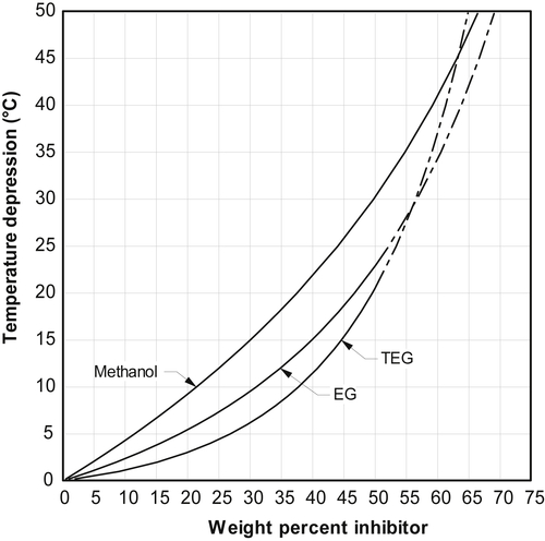
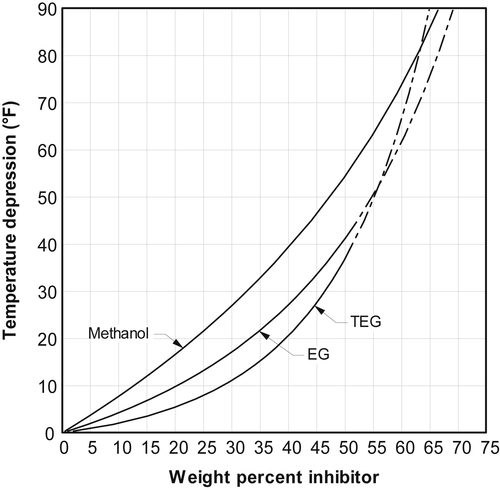
Admittedly, Eqn (5.10) is a little difficult to use, especially if the temperature depression is given and the required inhibitor concentration must be calculated. Therefore, a graphical version is presented in Fig. 5.4 in SI units and Fig. 5.5 in American engineering units. There are no experimental data for glycol concentrations greater than 50wt%, therefore, beyond this concentration, the correlation is an extrapolation.
From this chart, it is quite easy to determine the temperature depression for a given inhibitor concentration and vice versa.
Figure 5.4The Inhibiting Effect of Methanol, Ethylene Glycol (EG), and Triethylene Glycol (TEG)—SI Units.
Figure 5.5The Inhibiting Effect of Methanol, Ethylene Glycol (EG), and Triethylene Glycol (TEG)—American Engineering Units.
5.4.2. Accuracy of the New Method
The new equation is compared with some data from the literature. For convenience, and with apologies to the original authors, the original sources of the data are not listed. The data were taken from the monograph of Sloan (1999).
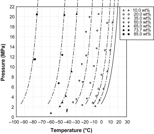
Figure 5.6 shows the calculated depression for the methane hydrate using methanol. The curves are for 10, 20, 35, 50, 65, 73.7, and 85wt% methanol. The new equation is shown to be very good even for these high methanol concentrations.
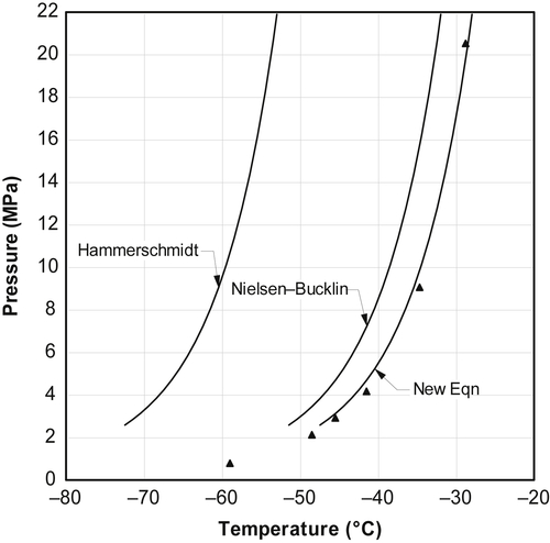
For comparison purposes, Fig. 5.7 shows only the 65wt% curve. However, included in this plot are the predictions from the Hammerschmidt and Nielsen–Bucklin equations. At this methanol concentration, the Hammerschmidt equation predicts a temperature depression that is about 28°C too large. The Nielsen–Bucklin equation is an improvement over the Hammerschmidt equation, but it is also overpredicts the inhibiting effect. The Nielsen–Bucklin equation is in error by about 4°C. In a practical sense, this means that the methanol injection rate predicted using either the Hammerschmidt or the Nielsen–Bucklin equations would be too small.
Figure 5.6The Inhibiting Effect of Methanol on the Methane Hydrate.(Curves from Eqn (5.10).)
Figure 5.7The Inhibiting Effect of 65wt% Methanol on the Methane Hydrate.
Figure 5.8The Inhibiting Effect of Ethylene Glycol on the Methane Hydrate.
Figure 5.8 shows the inhibiting effect of EG on the methane hydrate. Again, this figure demonstrates that the new equation is an excellent prediction of the experimental data.
Again, Fig. 5.9 is presented in order to compare the new equation with the correlations available in the literature. This figure is for 35wt% EG. The original Hammerschmidt equation does a surprisingly good job. However, the Gas Processors Suppliers Association (GPSA) modification grossly overpredicts the temperature depression. The GPSA equation is in error by about 6°C. Again, this translates to an EG injection rate that is too small for the desired inhibition.
5.5. Brine Solutions
As was mentioned earlier, ionic solids also inhibit the formation of hydrate in much the same way that they inhibit the formation of ice. Some quick rules of thumb can be found in the observations based on experimental measurements.
Maekawa (2001) measured hydrate formation for methane and a mixture of methane and ethane, although rich in methane, in both pure water and 3wt% NaCl for pressures from about 3 to 12MPa. His data show that the hydrate formation temperature was reduced by about 1°C for brine with this concentration. It is also demonstrated that the temperature depression is independent of the gas mixture studied.
Figure 5.9The Inhibiting Effect of 35wt% Ethylene Glycol on the Methane Hydrate.
Mei et al. (1998) measured the hydrate formation for a natural gas mixture in pure water and in solutions of various ionic salts and for pressures from about 0.6 to 2.5MPa. Their data for pure water were presented earlier. For NaCl and KCl, their data show that ΔT is fairly constant over the range of temperatures shown. For CaCl2, ΔT tends to increase with increasing temperature. The results of the study of Mei et al. (1998) are summarized in Tables 5.4 and 5.5.
The temperature depression for these data is independent of the concentration when expressed in either wt% or molality.
5.5.1. McCain Method
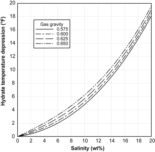
McCain (1990) provides the following correlation for estimating the effect of brine on the hydrate formation temperature:
ΔT=AS+BS2+CS3
(5.11)
where ΔT is the temperature depression in °F, S is the salinity in wt%, and the coefficients A, B, and C are functions of the gas gravity, γ, which is defined in Eqn (3.1), and are given below:
Table 5.4
Constants for the Østergaard et al. (2005) Correlation for the Inhibiting Effect of Ionic Solutions
Constant
NaCl
CaCl2
NaBr
c1
0.3534
0.194
0.419
c2
1.375×10⁻³
7.58×10⁻³
6.5×10⁻³
c3
2.433×10⁻⁴
1.953×10⁻⁴
1.098×10⁻⁴
c4
4.056×10⁻²
4.253×10⁻²
2.529×10⁻²
c5
0.7994
1.023
0.303
c6
2.25×10⁻⁵
2.8×10⁻⁵
2.46×10⁻⁵
Max. con. (mass%)
26.5
40.6
38.8
Max. con. (mol%)
10
10
10
Constant
K2CO3
KBr
KCl
c1
0.1837
0.3406
0.305
c2
−5.7×10⁻³
7.8×10⁻⁴
6.77×10⁻⁴
c3
2.551×10⁻⁴
8.22×10⁻⁵
8.096×10⁻⁵
c4
6.917×10⁻²
3.014×10⁻²
3.858×10⁻²
c5
1.101
0.3486
0.714
c6
2.71×10⁻⁵
2.3×10⁻⁵
2.2×10⁻⁵
Max. con. (mass%)
40.0
36.5
31.5
Max. con. (mol%)
8
8
10
Table 5.5
Constants for the Østergaard et al. (2005) Correlation for the Inhibiting Effect Polar Inhibitors
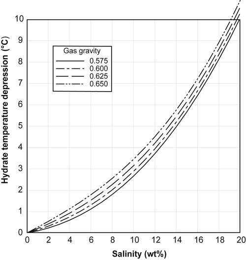
Equation (5.11) is limited to salt concentrations of 20wt% and for gas gravities in the range 0.55<γ<0.68. These equations were used to generate Figure 5.10 and 5.11, which is useful for rapid approximation of the inhibiting effect.
It is unlikely that anyone would add salt to the water in order to prevent hydrate formation. However, produced waters often contain brine and it is important to be able to estimate the effect of the brine in the produced water on the hydrate formation temperature.
Figure 5.10Depression of Hydrate Temperature Due to Brain (SI Units).
Figure 5.11Depression of Hydrate Temperature Due to Brine (American Engineering Units).
5.6. Østergaard et al
Østergaard et al. (2005) presented a correlation that was significantly different from its predecessors. First, they built an equation applicable to both inorganic salts (such as NaCl) and organic compounds (such as alcohols and glycols). Second, it includes the effect of pressure.
The correlation has the form:
ΔT=(c1W+c2W2+c3W3)(c4lnP+c5)(c6(P0−1000)+1)
(5.15)
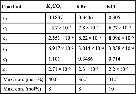
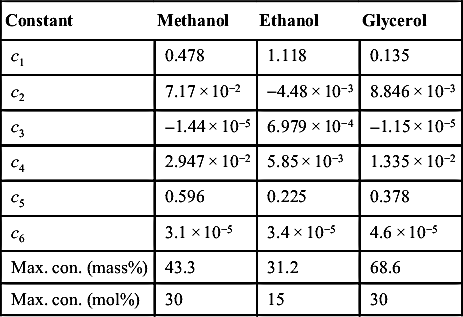
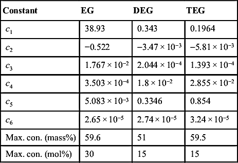
where ΔT is the temperature depression in K or °C, P is the pressure of the system in kPa, W is the concentration of the inhibitor in liquid water phase in mass%, P0 is the dissociation pressure of hydrocarbon fluid in pure water at 0°C in kPa, and the cis are parameters listed in Table 5.6. Also given in the tables is the stated range of applicability.
For solutions of ionic solids, the authors indicate that the average errors are less than 1.5% and for the polar inhibitors the average errors are slightly larger but still less than 2% for alcohols and glycols and about 5% for glycerol. On the other hand, the correlation is applicable over a wider range of concentrations when applied to the polar solvent as compared with the ionic solids.
Table 5.6
Hydrate Point Depression Observed by Mei et al. (1998) Due to Ionic Salts
wt%
mol%
Molality
Average ΔT
NaCl
10
3.31
1.90
5
KCl
10
2.61
1.49
3
CaCl2
10
1.77
1.00
4
The equation is simple to use if you know the inhibitor concentration and you want to estimate the depression. It is more difficult to use if the temperature is specified and you wish to calculate the required inhibitor concentration. This requires an iterative solution.
5.7. Comment on the Simple Methods
These simple methods, Hammerschmidt, Nielsen–Bucklin, and the new method developed for this book, have several characteristics in common. At this point, it is time to review some of them.
All of these simple methods predict the depression of the hydrate temperature; they do not predict the actual hydrate formation conditions. First, you must begin with the methods presented in Chapters 3 and 4 to predict the hydrate formation in the absence of the inhibitor. Then, you can use the methods presented earlier to correct for the presence of the inhibitor. Therefore, if your method for estimating the hydrate formation condition in the absence of inhibitor is a poor model, then the corrections noted in the first part of this chapter will also be inaccurate. These correction factors cannot overcome a poor original prediction.
Note that these methods assume that the inhibition effect is independent of the pressure. Experimental work indicates that this is nearly the case. To within a good engineering estimate, it is safe to neglect the effect of pressure on the inhibiting effect.
Furthermore, these methods assume that the temperature depression is independent of both the nature of the hydrate former present and the type of hydrate formed. So the temperature depression in a 25wt% methanol solution is the same for a methane hydrate (type I) as it is for a propane hydrate (type II).
There is a little bit of confusion about the units on the quantity calculated via these methods. The result obtained is a temperature difference, not an actual temperature. Therefore, if you calculate a ΔT of 5°C, to convert this to Fahrenheit, simply multiply by 1.8 to get 9°F. You do not convert the 5°C to 41°F as if it were a temperature reading.
5.8. Advanced Calculation Methods
Just as there were more advanced methods for calculating hydrate formation conditions, there are more rigorous methods for estimating the effect of inhibitors (for example, see Anderson and Prausnitz (1986)). As with most rigorous methods, these methods are suited for computer calculations and not for hand calculations.
The van der Waals–Platteeuw-type models discussed in the previous chapter can be extended as follows:
where xW is the mole fraction of water and γW is the activity coefficient of water in the aqueous solution. The bar over the temperature in the last term in the above equation indicates that this is an average temperature. The activity coefficient of water can be modeled using the equations commonly used for vapor–liquid equilibrium.
As a contrast to the simple model, these advanced models can and do account for the variables that are neglected in the simple models. For example, these models do include the effect of pressure and the type of hydrate.
5.9. A Word of Caution
Methanol is very useful for combating the formation of hydrates in pipelines and process equipment. However, methanol can have an adverse effect on subsequent processing of the hydrocarbon stream.
As an example of a processing problem that may arise with methanol use, it is possible that methanol will concentrate in the liquefied petroleum gas (LPG) stream. LPG is made up largely of propane and mixed butanes. It is known that propane+methanol and n-butane+methanol form azeotropes (Leu et al., 1992). These azeotropes mean that it is impossible to separate the systems using binary distillation. In a practical sense, this is why methanol may appear in unacceptable amounts in the LPG product.
In addition, methanol-hydrocarbon systems are notoriously difficult to model accurately. However, applied thermodynamics has made great strides in this area. The design engineer should be cautious about the models chosen to perform calculations on such systems.
Another interesting side-effect of methanol use is on corrosion inhibitors. At one site, methanol was injected into a pipeline to prevent hydrate formation. Inhibitor chemicals were also injected to prevent corrosion. The inhibitors were alcohol based and the methanol dissolved the inhibitor. This led to some unexpected corrosion problems.
Another potential corrosion problem related to methanol injection is dissolved air in the methanol. Methanol for inhibitor is usually stored on site in tanks that are open to the atmosphere. This allows some air to dissolve into the methanol. Then, upon injection into a process or pipeline, it may cause corrosion problems. Typically, the amount of dissolved oxygen is small, but over the long term this could cause problems.
5.10. Ammonia
Ammonia was once suggested as an inhibitor for hydrate formation. It has a relatively low molar mass, 17.03g/mol vs 32.04g/mol for methanol, which as we have seen is advantageous for an inhibitor. Based on the Hammerschmidt equation, a 10°C depression in the hydrate formation temperature requires an 11.6wt% ammonia solution vs a 19.8wt% methanol solution.
Ammonia may be more useful in thawing hydrate plugs in pipelines. Unlike liquid inhibitors, which require pressure drop in order to flow to reach a plug—typically not available in a plugged line—ammonia can diffuse through the gas phase to reach the hydrate plug.
Unfortunately, ammonia has several drawbacks as well. It is toxic and may be difficult to handle in oil filled applications. In addition, it reacts with both carbon dioxide and hydrogen sulfide in the aqueous phase.
Ammonia's volatility is a disadvantage as well as an advantage. Its high volatility translates into larger losses to the vapor.
The disadvantage outweighs any possible advantage and, therefore, ammonia is rarely (perhaps never) used as a hydrate inhibitor.
5.11. Acetone
Nature is interesting in that she always seems to provide exceptions to the rules. In the field of hydrate inhibition, one exception is acetone. Acetone is a polar compound that is liquid at room temperature. It shares many characteristics in common with alcohols and would appear at first glance to be an excellent candidate for use a hydrate inhibitor. Closer scrutiny demonstrates that this is not the case.
In all honesty, no one would probably suggest using acetone as a hydrate inhibitor. Compared to methanol, it is more costly and is predicted to be less effective. For example, the Hammerschmidt equation indicates that, for a given weight fraction of inhibitor, the temperature depression is inversely proportional to the molar mass of the inhibitor. The molar mass of acetone (58.05g/mol) is almost twice that of methanol. Therefore, for a given weight percent, the temperature depression from acetone would be approximately half that for methanol.
The reason that acetone was suggested for this application was that a company had a waste stream composed of methanol, ethanol, and acetone and wished to examine it as a potential hydrate inhibitor. It turned out that the blend performed much worse than anticipated and the culprit was the acetone. At low concentrations, the acetone enhanced the hydrate formation rather than depressed it. That is, for a given pressure, the hydrate in an acetone solution formed at a higher temperature than in pure water. Only at high concentrations did the acetone begin to inhibit the formation of the hydrate. More details of this work can be found in Ng and Robinson (1994). Confirmation of this unusual result was obtained by Mainusch et al. (1997). These experiments were conducted for the methane hydrate, but similar results could be anticipated for other hydrate formers.
Mainusch et al. (1997) were able to model the phenomenon but no detailed explanation was provided. That is, the role of the acetone in hydrate formation is unclear. Is acetone a hydrate former (i.e., does it enter the cages)? Is acetone a host (i.e., does it form part of the crystal lattice along with the water molecules)? Or does it play some other role?
5.12. Inhibitor Vaporization
Methanol is a volatile substance and, thus, when it is injected into natural gas and/or condensate some of the methanol will enter these phases. In practical terms, this means that more inhibitor must be injected than the amount predicted solely from the aqueous phase concentrations. If only that amount of inhibitor is injected, then not enough will be used.
The inhibitors are volatile and, thus, will evaporate from the aqueous liquid where they are required to inhibit the hydrate formation to the vapor. Some inhibitors are more volatile than others. The vapor pressures of some common inhibitors are plotted in Fig. 5.12.
Figure 5.12Vapor Pressures of Common Inhibitor Chemicals and Water.
Fortunately, there are charts available for estimating these losses. Figures 5.13 and 5.14 can be used to estimate the amount of methanol dissipated in the natural gas. These charts are approximations and should be used with care, especially if used for design.
The chart for the methanol losses to the vapor is a little confusing. The abscissa (x-axis) has units of kgMeOH(106Sm3)(wt%MeOH) in SI units or lbMeOH(MMCF)(wt%MeOH) in American engineering units. To calculate the methanol in the vapor locate the point that corresponds to the pressure (ordinate) and temperature (third parameter), and then read the value off the x-axis. The value on the x-axis is multiplied by the gas rate and the aqueous phase methanol concentration to get the methanol rate in the vapor. For example, at 9°C and 5000kPa, the value from the abscissa is 25. If the gas rate is 50×103Sm3/day and the aqueous phase concentration is 35wt%, then the methanol in the gas is 25×(50×103/106)×35=43.75kg/day.
From this chart, we can make some general observations. First, for a given temperature, the methanol losses increase with decreasing pressure. Second, at constant pressure, the losses increase with increasing temperature. In addition, the higher the gas rate, the higher the methanol losses to the vapor. Finally, the higher the methanol concentration in the aqueous phase, the greater the losses to the vapor. All of these are somewhat intuitive observations.
Figure 5.13The Ratio of Methanol Vapor to the Methanol in the Aqueous Liquid as a Function of Pressure and Temperature in SI Units.Reprinted from the GPSA Engineering Data Book, 11th ed.—reproduced with permission.
Figure 5.14The Ratio of Methanol Vapor to the Methanol in the Aqueous Liquid as a Function of Pressure and Temperature in American Engineering Units.Reprinted from the GPSA Engineering Data Book, 11th ed.—reproduced with permission.
To use these charts to estimate the methanol in the nonaqueous phase, first one estimates the amount of methanol required using the methods outlined earlier. From that point, one can estimate the amount of methanol present in the other two phases. Only from this can the total amount of methanol injected can be calculated.
The glycols are much less volatile than methanol. In addition, glycols are usually used at low temperature. Thus, losses to the nonaqueous phases are less of a concern when using glycols.
Usually, the engineer will calculate the amount of inhibitor (usually methanol) that must be injected in order to avoid hydrate formation. This value is then passed along to field operations. The field operators will often adjust this value in order to minimize costs while still ensuring problem-free production.
5.12.1. A More Theoretical Approach
A crude estimate of the inhibitor losses to the vapor can be estimated assuming that Raoult's Law applies and that the nonidealities in the vapor phase can be neglected. This leads to the simple equation:
yi=xi(PsatiP)
(5.17)
where yi is the mole fraction of the inhibitor in the vapor phase, xi is the mole fraction in the aqueous phase, Psati is the vapor pressure of the inhibitor, and P is the total pressure. Rearranging this equation to more familiar units (and units that will be used later), we obtain the following equation in SI units:
Yi=(760.4XiMi100Mi−[Mi−18.015]Xi)(PsatiP)
(5.18)
where Yi is the inhibitor in the vapor phase in kg/MSm3, Xi is the weight percent inhibitor in the aqueous phase, and Mi is the molar mass of the inhibitor. In American engineering units, the equation is:
Yi=(47484XiMi100Mi−[Mi−18.015]Xi)(PsatiP)
(5.19)
where Yi is the inhibitor in the vapor phase in pounds per million standard cubic feet (lb/MMCF), Xi is the weight percent inhibitor in the aqueous phase, and Mi is the molar mass of the inhibitor. With the appropriate properties, this equation can be used for any nonionic inhibitor.
Although this is an over simplified method, somewhat more accurate methods will be presented later, we can make some observations based on this equation. As the temperature increases, the vapor pressure increases and, thus, inhibitor losses increase.
Based on this simple analysis, the losses from methanol are about 2.5 times as large as ethanol, and about 200 times that for EG. TEG is even less volatile and losses are negligible.
Comparing this equation to the chart method reveals a potential correction. It can be seen that the error in the estimate from the equation increases with increasing pressure.
Yi=Cf(760.4XiMi100Mi−[Mi−18.015]Xi)(PsatiP)
(5.20)
or
Yi=Cf(47484XiMi100Mi−[Mi−18.015]Xi)(PsatiP)
(5.21)
where Cf is given by the following equation in SI units:
Cf=1.1875+1.755×10⁻⁴P
(5.22)
where Cf is unitless and P is in kPa. In American engineering units, this equation becomes:
Cf=1.1875+1.210×10⁻³P
(5.23)
where P is in psia. This is a purely empirical correction and there is no thermodynamic basis for making such a correction. Therefore, extrapolations outside the range of pressure and temperature should be done with caution.
5.12.2. Inhibitor Losses to the Hydrocarbon Liquid
In addition to the loss of inhibitor to the gas, if a liquid hydrocarbon is present, some of the inhibitor will enter that phase too. This section provides methods for estimating the loss of inhibitor to the condensate.
5.12.2.1. Methanol
The GPSA Engineering Data Book gives a chart for the distribution of methanol between a liquid hydrocarbon (condensate) and an aqueous solution reproduced here as Fig. 5.15. This chart is basically a plot of the raw experimental data. Figure 5.16 is a similar plot with some smoothing. Although the estimated values from the two charts are not the same, they are suitable for engineering calculations.
The chart is a plot of the mole fraction in the hydrocarbon liquid as a function of the temperature and the methanol concentration in the water rich phase. Using this chart for a given application requires the molar mass of the hydrocarbon liquid. Unfortunately, there is no typical value for the molar mass. For light condensate, it could be as low as 125g/mol and for heavier oils it may be as large as 1000g/mol.
For weight fractions between 20 and 70wt%, it is sufficiently accurate to “eye ball” your estimate. For methanol concentrations less than 20wt%, a linear approximation can be used, given the fact that at 0wt% in the water the concentration in the hydrocarbon liquid is also 0. The resulting equation is:
x=x(20wt%)20X
(5.24)
where X is the given weight percent methanol in the aqueous phase, x (20wt%) is the mole percent methanol in the condensate at 20wt% in the water, and x is the mole fraction in the hydrocarbon liquid for the given X. This equation applies to both SI and American engineering units.
Figure 5.15The Solubility of Methanol in Paraffinic Hydrocarbons as a Function of Aqueous Phase Composition, Pressure, and Temperature in SI Units.Reprinted from the GPSA Engineering Data Book, 11th ed.—reproduced with permission.
Figure 5.16The Solubility of Methanol in Paraffinic Hydrocarbons as a Function of Aqueous Phase Composition, Pressure, and Temperature in American Engineering Units.Reprinted from the GPSA Engineering Data Book, 11th ed.—reproduced with permission.
The data of Chen et al. (1988) indicate that the methanol losses increase if the hydrocarbon liquid is aromatic. In an aromatic-rich condensate, the methanol losses could be as much as five times those in a paraffinic condensate.
Note the chart shows no effect of pressure on the distribution of methanol between the two liquid phases. This is common for liquid–liquid equilibrium and probably a good assumption in this case.
5.12.2.2. Glycol
A small amount of experimental data in the temperature range from −10 to 50°C (14 to 122°F) indicate that the EG in the hydrocarbon liquid is about at least 100 times less than the methanol, when expressed in terms of mole fraction. Based on these observations, it is probably safe to assume that EG losses to the condensate are negligibly small.
TEG losses to the condensate are just as small as those for EG.
5.13. A Comment on Injection Rates
Methanol injection rates of 0.15–1.5m3/day (1–10bpd) are common in the natural gas business. Occasionally, they may be more than this, but injection rates of more than 1.5m3/day become rather expensive. In oil field terms and from a cost point of view, these seem like relatively large numbers. In reality, they are very small rates. For example, 0.15m3/day converts to only 0.1L/min (0.026gpm) or 1.7mL/s. A drop of liquid is approximately 0.5mL in volume. Therefore, the injection rate is only three drops per second.
Another aspect of inhibitor injection is that often it is at high pressure. Injection pressures greater than 7000kPa (1000psia) are common.
Therefore, the injection pump must be designed to handle these conditions—low rates and high pressures. Fortunately, there are such pumps available. Two types are common (1) a diaphragm pump and (2) a piston pump. Both types work quite well for this application.
5.14. Safety Considerations
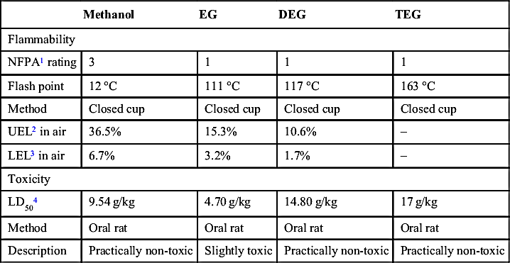
Table 5.7 lists some of the properties of methanol and the glycols from a safety point of view. Methanol is often used as a fuel and hence it is well known that this alcohol is flammable. This is reflected in the relatively high National Fire Protection Association (NFPA) rating. The glycols are significantly less flammable. Thus, from a fire prevention point of view, the storage of methanol is considerable more dangerous than that for glycols. The fire hazard of methanol vs glycol may be more significant in confirmed spaces such as on an offshore rig.
Both methanol and glycols are potential toxins if consumed in large enough quantities. Extrapolating the values for rats to a 70kg (154lb), for a human it indicates that about 670g of pure methanol must be consumed for an LD50. This is equal to slightly less than 1L (about 1 US quart). This is strictly not how these values should be interpreted, but it gives an indication of the toxicity.
Another problem with the glycols is that they have a sweet flavor, which is attractive to children and some animals.
5.14.1. Diluted Methanol
For safety reasons, some companies do not store pure methanol at their well sites, batteries, plants, etc., choosing to store only diluted methanol. Typically, this would be less than 50wt% and often much less. If the methanol injected on-site is diluted, this will require additional methanol to be injected.
Table 5.7
Properties of Various Hydrate Inhibitor and Dehydration Chemicals from a Health and Safety Point of View
4LD50—LD stands for “Lethal Dose.” LD50 is the amount of a material, given all at once, which causes the death of 50% (one half) of a group of test animals. The LD50 is one way to measure the short-term poisoning potential (acute toxicity) of a material. In general, the smaller the LD50 value, the more toxic the chemical is.
There is another problem with using diluted methanol. The concentration of the stored methanol puts an upper limit on the concentration attainable in the pipeline. If the stored methanol is 25wt%, how can you achieve 50wt% if that is required based on the hydrate considerations? No matter how much 25wt% is injected, a concentration of 50wt% will never be achieved.
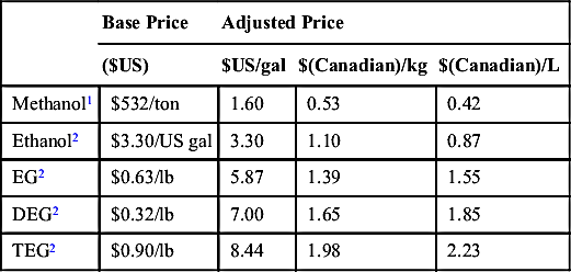
5.15. Price for Inhibitor Chemicals
Table 5.8 gives the approximate cost of chemicals that are used for inhibiting hydrate formation.
As can be seen from Table 5.8, the cost of glycol is significantly greater than methanol. Thus, it is usually cost-effective to recover the injected glycol. Usually, the methanol is injected and not recovered. Although it is cost-effective to recover the injected glycol, one reason why this is usually not done is that the produced water is usually a brine. In the regeneration of the glycol, the salt is concentrated in the glycol, which ultimately causes processing problems.
New hydrate inhibitors have entered the market that are markedly different from the thermodynamic inhibitors. The thermodynamic inhibitors are the alcohols, glycols, and ionic salts discussed earlier in this chapter. These basically inhibit the hydrate formation by depressing the freezing point—a thermodynamic effect.
The inhibition of hydrates using methanol or glycol is thermodynamic inhibition. The purpose of the addition of these chemicals is to shift the equilibrium to lower temperatures and higher pressures, thus reducing the region where hydrates can exist.
The new inhibitors, the so-called low-dosage hydrate inhibitors are in two classes: (1) kinetic inhibitors and (2) anticoagulants. They are called low dosage because, as we shall see, they can be used in significantly lower concentrations than the thermodynamic inhibitors.
Many of these new chemicals are patented. The appendix to this chapter gives a partial list of patents relating to low-dosage inhibitors. This is not meant to be an exhaustive list nor does it include any details from the patents.
5.16.1. Kinetic Inhibitors
Recently, there has been a class of chemicals developed called “kinetic inhibitors” or KHIs. Basically, the purpose of this type of inhibitor is to prevent the hydrate from crystallizing. In other words, its purpose is to slow the process by which the hydrate crystallizes. These chemicals delay hydrate formation and growth such there is sufficient time to transport the fluids to their destination. However, given sufficient time, hydrates will form even in the presence of the KHI.
Furthermore, it has been found that such chemicals can be used in very small concentrations. For example, according to Fu et al. (2001), these inhibitors can depress hydrate formation by 11°C (20°F) at concentrations less than 3000ppm.
The chemicals that have been examined for this purpose are usually polymers and therefore are of high molar mass. In addition, they are water soluble (or at least have significant water solubility).
In recent years, there have been several successful field trials of these chemicals, examples include:
1. Fu et al. (2001) describe one trial for a 135mile long, 4-in flow line transported between 11 and 15 million standard cubic feet per day (MMSCFD) of gas and 13bpd of produced water, with a salinity of 6wt% dissolved solids. Prior to the KHI test, methanol was injected at a rate of between 150 and 220gallons per day. A new program was developed to inject a KHI at an effective concentration of 550ppm polymer (an injection rate of 3gallons per day of blended chemical). In the time period reported (more than 1year), there were no hydrate incidents reported. It is reported that the switch from methanol to KHI results in a chemical cost savings of about 40%.
3. Glenat et al. (2004) describe the application of KHI in the offshore flow lines operating at pressures greater than 1000psia (7MPa) South Pars field in Iran.
5. Hagen (2010) describes three case studies using KHI in British Columbia and Alberta, Canada.
a. This location in British Columbia is accessible by road only during the winter months. Thus to get methanol to the location during other times it had to be flown by helicopter, which was expensive. A switch was made to a mixture of methanol and KHI. This change reduced the demand for chemicals and flying them in was no longer necessary. The chemical could be delivered during the winter months when the roads were passable.
b. This producer had a flow line transporting, on average, 10m3/day of oil and 400×103Sm3/day of sweet gas. The water rate was estimated to be 1m3/day but was not metered so the exact rate was not known. The line required approximately 600L/day of methanol for hydrate prevention. After a review, the methanol was replaced by a KHI+methanol (10%) blend. The initial rate was set to 250L/day and there were no issues with hydrates.
c. In this case, the water, liquid hydrocarbons, and gas were separated and the gas was transported via a pipeline. The gas entered the line at a rate of about 100×103Sm3/day. The gas is water saturated when it enters the line and is slightly sour containing about 2000ppm of H2S. Methanol was injected at a rate of about 64L/day. Although there was no plugging because of hydrate formation, they were found during pigging operations. The treatment scheme was changed to a blend of a KHI and methanol. The initial rate for the blend was 10L/day, but it was optimized to 6L/day. Hydrates are no longer observed during pigging of the line.
5.16.2. Anticoagulants
Anticoagulant (also called anti-agglomeration) inhibitors work on a different level. They do not prevent hydrate formation, but they prevent the accumulation of hydrate into a plug. The hydrate stays in a slurry, which can still be transported and will not plug the line.
The use of an anticoagulants implies the transport of a slurry product. Sinquin et al. (2004) provided an interesting and thorough study of the rheology of hydrate slurries. The particles formed in the fluid modifies the flow properties. In the turbulent regime, pressure drop is controlled by the friction factor, whereas in the laminar regime, it is due to changes in the apparent viscosity.
Field application of anticoagulants have been described in the literature. Brief descriptions of a few applications are provided below:
1. Thieu and Frostman (2005) described an application at a field producing 8MMSCFD of gas, 220bpd of oil, and about 3bpd of water. The operator was injecting about 170gal/day of methanol, but still had hydrate problems. They switched to a regime that included the injection of 4gal/day of an anticoagulant and initially 27gal/day of methanol. Subsequently, the methanol coinjection was terminated.
2. Cowie et al. (2003) described the application of an anticoagulant's inhibitor on an offshore project in Louisiana. Production includes 65,000bpd of oil, 68MMSCFD of gas, and water that is transported to the processing facilities via a 41-mile long, 12-inch diameter pipeline.
3. Klomp et al. (2004) described the application of an anticoagulant's inhibitor in a region of the Dutch North Sea. The field produces gas, a waxy crude oil, and water.
4. Hagen (2010) described two case studies using anticoagulant in Alberta, Canada.
a. A well producing 9m3/day of brine, 36m3/day of oil, and 4×10³Sm3/day of sour gas. The fluids were transported 9km. Methanol injection was up to 6000L/day and still hydrates formed. A program was started to inject AA and the rate was optimized to 90L/day without hydrate plugging.
b. At this site, the typical production was 2m3/day of water, 3.5m3/day of oil, and 0.5×10³Sm3/day of gas. The injection rate for the AA was adjusted to about 15L/day, which corresponds to a concentration of about 1750ppm in the aqueous phase, and no hydrate blockages were noted through a winter season.
Examples
Example 5.1
Calculate the freezing point of a 10% solution of methanol in water.
The reader should verify that the units are correct. Therefore, the freezing point of the mixture is estimated to be −6.5°C.
Example 5.2
The methane hydrate forms at 15°C and 12.79MPa (Table 2.2). Calculate the amount of methanol required to suppress this temperature by 10°C using the Hammerschmidt equation.
Answer: The molar mass of methanol is 32.042g/mol. From Eqn (5.4) we have:
This is outside the range of this correlation, so this result should be taken with some trepidation. However, it demonstrates that significantly more EG is required, when expressed as weight fraction, because of its significantly higher molar mass.
Answer: From Fig. 5.4, to get a 10°C depression in the hydrate formation temperature using methanol requires 21wt% methanol and 31wt% EG. In this case, there is good agreement between the chart and the Hammerschmidt equation.
Example 5.5
From Fig. 5.1, it can be estimated that the hydrate formation temperature of hydrogen sulfide is depressed by 18°C in 35wt% methanol and by 25°C in 50wt% methanol. Compare this to the values predicted by (1) the Hammerschmidt equation, (2) the Nielsen–Bucklin equation, and (3) Fig. 5.4.
Answer: (1) From the Hammerschmidt equation for 35wt%, we get:
ΔT=1297(35)/(34.042)(100−35)=20.5°C
and for 50wt%:
ΔT=1297(50)/(34.042)(100−50)=38.1°C
These are in error by 14% and 52%, respectively. Actually, the 35wt% answer is closer than anticipated.
(2) To use the Nielsen–Bucklin equation, we must convert to mole fraction. For methanol, 35wt%=23.6mol% and 50wt%=36.0mol%. The readers can verify these conversions for themselves. Now, for the 35wt% we get:
ΔT=−72ln(1−0.236)=19.4°C
and for the 50wt%:
ΔT=−72ln(1−0.360)=32.1°C
These represent errors of 8% and 28%, respectively. Although the estimate for the 50wt% mixture is an improvement over the Hammerschmidt equation, it is not as accurate as we would like considering the Nielsen–Bucklin equation is reputed to be accurate for greater concentrations than these.
(3) From Figure 5.4, you can read from the chart that 35wt% gives a depression of 18°C and 50wt% is about 30°C, which are errors of 0% and 20%, respectively. These values are improvements over both the Hammerschmidt and Nielsen–Bucklin equations.
Part of the reason for the inaccuracy of all of the methods may be the fact that we are dealing with hydrogen sulfide, which behaves significantly differently than sweet gas. For one thing, H2S is more soluble in water than are the hydrocarbons. Furthermore, the solubility of H2S in methanol, and hence aqueous solution, is even larger. This solubility has an effect on the hydrate depression.
Example 5.6
Natural gas is to be transported from a well site to a processing plant in a buried pipeline at a rate of 60×103m3[std]/day. The production also includes 0.1m3[std]/day of water, which is to be transported in the same pipeline. The gas enters the pipeline at 45°C and 3500kPa. The hydrate formation temperature of the gas is determined to be 40°C at 3500kPa. In the transportation through the pipeline, the gas is expected to cool to 8°C. Calculate the amount of methanol that must be injected in order to prevent hydrate formation.
Answer: First, calculate the required temperature depression.
ΔT=40−8=32°C
Include a 3°C safety factor, the required temperature depression is 35°C.
Now use Eqn (5.4) to estimate the concentration of methanol required.
This is outside the range of applicability of the Hammerschmidt equation. The value obtained from Fig. 5.4 is 55wt%, which is both a better estimate and significantly larger than the Hammerschmidt estimate. We will use 55wt% for the rest of this calculation.
Next, we calculate that 0.1m3 of water has a mass of about 100kg. Therefore, to get a 55wt% solution, based on water+methanol and not the entire stream, requires the injection of 122kg/day of methanol. The density of methanol is 790kg/m3, so the methanol is injected at a rate of 0.155m3/day or 155L/day.
If we used the values of 46.4wt% from the Hammerschmidt equation, this converts to an injection rate of 86.6kg/day.
Note, the amount of water in the natural gas (because it is being produced with free water, we can assume that it is saturated with water), has been neglected in this calculation. It is left to the reader to calculate the amount of water in the gas and determine if additional methanol is required to account for this water.
Example 5.7
Estimate the amount of methanol required to saturate the gas in Example 5.6, and from that determine the total amount of methanol that must be injected.
Answer: Using Fig. 5.12, we can read that at 8°C and 3500kPa, the methanol in the vapor is 27kgMeOH(106Sm3)(wt%MeOH).
In the previous example, we determined that the aqueous phase concentration should be 55wt%. Therefore, the amount of methanol in the vapor is:
27×(60×103Sm3/106)×(55wt%)=89.1kg/day
which converts to 0.113m3/day or 113L/day.
Therefore, the total methanol requirement is 155+113=268L/day. At this point, it is worth noting that 42% of the methanol injected will vaporized. Therefore, instead of the 155L/day injection rate, which is based only on the aqueous phase, the actual injection rate that is required is more than 1.7 times that amount.
Example 5.8
Estimate the cost of the methanol injection from Example 5.7.
Answer: From the earlier calculation the injection rate was 268L/day, so 268L/day×$0.27 (Canadian)/L=$72 (Canadian)/day or about $26,000 (Canadian)/year or $17,300 (US)/year.
Example 5.9
Natural gas flowing in a pipeline exits the line at 45°F and 700psia and the flow rate of the gas is 5MMSCFD. In order to prevent hydrate formation, it is estimated that there should be 25wt% methanol in the aqueous phase. Calculate the methanol losses to the vapor phase (1) using the simple equation (Eqn (5.19)), (2) using the corrected equation (Eqn (5.21)), and (3) using the chart (Fig. 5.13). (4) Estimate the concentration of methanol in the condensate, if condensate were present.
Answer: (1) At 45°F, the vapor pressure of methanol is 0.92psia. From the simple equation:
Based on this correction factor, the simple equation underestimates the methanol losses by a factor of two. In other words, the actual losses will be twice those estimated using the simple equation.
Yi=(2.035)(17.65)=35.92lbMeOH/MMCF
and the total methanol loss is (35.95)(5)=179.75lb/day=7.5lb/h.
(3) From the chart, Y/X=1.4, therefore, Y=1.4(25)=35lb MeOH/MMCF. Again multiplying by the gas flow rate gives (35)(5)= 175lb/day=7.3lb/h. The agreement between the corrected equation and the chart is very good in this case.
(4) Estimate the concentration of the methanol in the condensate at 30°F if the methanol concentration in if the water phase is 15wt%.
From the chart, the methanol concentration in the condensate at 20wt% is 0.07mol%. Then using the following equation:
x=x(20wt%)20X=(0.07)(15)20=0.053mol%
Example 5.10
Assuming a water flow rate of 1bpd and methanol needs to be injected to have a 25wt% solution in order to assure hydrates will not form in the pipeline.
1. How much pure methanol must be injected to achieve the goal of 25wt%?
2. If the methanol is available with a concentration of 30wt%, how much solution must be injected to achieve the goal of 25wt%? How much of this solution is methanol?
Answer: First, 1bpd of water is 42gal/day. The density of water is 8.34lb/gal and, thus 42×8.34=350lb/day. This result is necessary for both parts of this question.
1. In order to have 25wt%, which is 0.25 mass fraction, let x be the mass of methanol injected. Then from a simple ratio:
0.25=x/(x+350)
Solving for x gives 117lb/day of pure methanol.
2. In this case, let x be the amount of solution injected. This time the ratio is:
0.25=0.3x/(x+350)
solving for x gives 1750lb/day of 30wt% methanol. This in turn means 0.3×1750 or 525lb/day of methanol are injected. Because the methanol is injected in dilute form, and water is added to the system, more total methanol needs to be injected.
Example 5.11
Assume a protein that inhibits the formation of ice is in the blood of an animal. Further assume that this inhibition is simply a freezing point depression. Estimate the concentration of the protein in order to achieve a 0.5°C depression. Typically, these proteins are high molecular weight (greater than 2500g/mol), so assume a value of 2500g/mol.
Answer: Begin with the freezing point depression equation:
It would seem highly unlikely that the protein would be 40wt% of the blood, so freezing point depression is unlikely to account for the observed reduction in the freezing point.


 (5.1)
(5.1) (5.2)
(5.2)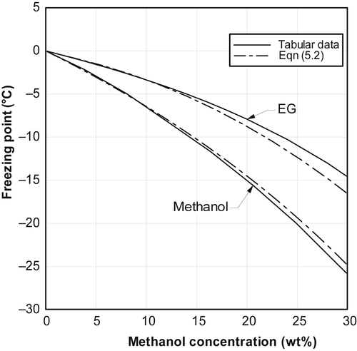
 (5.3)
(5.3)
 (5.6)
(5.6) (5.7)
(5.7)


 (5.16)


 (5.17)
 (5.18)
 (5.19)
 (5.20)
 (5.21)