
Chapter 9
Phase Diagrams
Abstract
Phase diagrams are a tool that engineers can use to resolve problems, not only with hydrates but with other phases as well. To begin, this chapter presents some rules for constructing phase diagrams. Several specific examples are then presented and some interesting results are revealed. For example, using phase diagrams it is demonstrated that free-water is not required for hydrates to form. Another extreme case is also demonstrated – excess water can inhibit hydrate formation.
Keywords
Phase envelopes; Pressure-composition diagrams; Pressure-temperature diagramsPhase diagrams are useful for both the theoretical discussion of gas hydrates and for engineering design. In this chapter, we will concentrate on fluid phase equilibria as they relate to hydrate formation. Thus, systems that do not form hydrates will not be discussed. This does not mean that they are not interesting or important, just beyond the scope of this book.
In this chapter, some rules are presented for constructing pressure-temperature (P-T) diagrams for single component systems and binary systems as well as pressure-composition (P-x) and temperature-composition (T-x) diagrams for binary systems. These rules can be found throughout this chapter.
9.1. Phase Rule
Much of this material is based on the Gibbs phase rule. The phase rule is:
![]() (9.1)
(9.1)
where F is the degrees of freedom, N is the number of components, and p is the number of phases.
An example of its use is as follows: a single component existing in two phases would have 1 degree of freedom. That means that there is one independent variable to “play with.” Once one variable is fixed, all of the others are fixed as well. For example, a single component existing as a vapor and a liquid has one degree of freedom. If the temperature is specified, then there are zero degrees of freedom – the pressure is fixed. This pressure is called the vapor pressure.
9.2. Comments about Phases
There are some general observations about phases that are useful for developing phase diagrams. The first of these is that gases are always miscible. Therefore, a system, regardless of the number of components, cannot contain two vapor phases. Some may argue that at extreme conditions, two gas phases may exist, but these are dense phases and it may be more logical to treat one of these as a liquid. In addition, such phenomena usually occur beyond the range of temperature and pressure, which is of interest to those in the natural gas business.
A pure component has only one liquid phase. Thus, a single component cannot exhibit liquid phase immiscibility. Binary and multicomponent systems can and do exhibit liquid phase immiscibility. For example, it is common knowledge that oil and water do not mix.
A critical point is a point where the properties of the coexisting phases become the same. Critical points exist when a vapor and a liquid are in equilibrium and when two liquids are in equilibrium. The first critical point is the usual critical point, which should be familiar to natural gas engineers. The second type of critical point is usually called a consolute point.
Another common critical point occurs when two phases become critical while in the presence of a third phase. It may be a bit of a misnomer, but these points are called three-phase critical points.
It is also theoretically possible for three phases to simultaneously become critical (for example a gas and two liquids). Such a point is called a tricritical point.
On the other hand, a pure component can have more than one solid phase. For example, sulfur has two solid forms – rhombic and monoclinic. Carbon also exhibits three solid phases – the common diamond and graphite phases and the more recently discovered buckminsterfullerenes (the so-called “bucky balls”). Water has many different solid forms (denoted ice I, ice II, etc.), but most of these occur at extreme conditions (that is, at very high pressures).
9.3. Single Component Systems
For a pure component system, we are only interested in the P-T diagram. Actually, we are primarily concerned with how the single component information relates to the two-component systems.
The first rule about phase diagrams pertains to a one-component system existing as a single phase. The phase rule (N = 1 and p = 1) says that there are two degrees of freedom. Therefore, we present the following:
1. A single component system in a single phase occupies a region in the temperature-pressure plane.
This leads to the second rule. The phase rule for a single component system (N = 1) and two phases in equilibrium (p = 2) indicates that there is one degree of freedom.
2. For a single component system, the location where two phases are in equilibrium corresponds to a curve in the temperature-pressure plane.
The curve where vapor and liquid are in equilibrium is called the vapor pressure curve. If the component does not decompose, then this curve ends in a critical point. The solid–liquid curve is called the melting curve and the gas–solid the sublimation curve.
These curves bound the various single-phase regions. For example, the vapor region lies at pressures less than and temperatures greater than the vapor pressure curve and at temperatures greater that and pressures less than the sublimation curve.
The next rule arises when there are three phases in equilibrium. In this case, the phase rule says there are zero degrees of freedom. Thus, this is a fixed point in the P-T plane and is called a triple point. The location of the triple point is at the intersection of the two-phase loci.
3. Three two-phase loci intersect at a triple point, a point where three-phases are in equilibrium.
As a corollary to rule 3, the vapor pressure, melting, and sublimation curves intersect at a vapor-liquid-solid triple point. This is the most common triple point, but because multiple solids can exist, there may be other triple points. However, there cannot be a single component liquid-liquid-vapor triple point, because, as was stated earlier, two liquid phases cannot exist for a pure component.
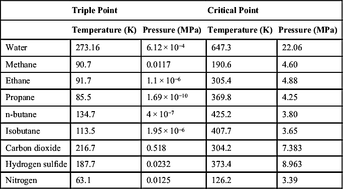
The critical points of components found in natural gas are listed in Table 9.1. This table also lists the vapor-liquid-solid triple points for these substances. Critical points for pure components are fairly well established and large tabulations are available. One reason for this is that the critical point is an important parameter in the correlation of fluid properties.
Table 9.1
Critical and Triple Points for Common Natural Gas Components
| Triple Point | Critical Point | |||
| Temperature (K) | Pressure (MPa) | Temperature (K) | Pressure (MPa) | |
| Water | 273.16 | 6.12 × 10⁻⁴ | 647.3 | 22.06 |
| Methane | 90.7 | 0.0117 | 190.6 | 4.60 |
| Ethane | 91.7 | 1.1 × 10⁻⁶ | 305.4 | 4.88 |
| Propane | 85.5 | 1.69 × 10⁻¹⁰ | 369.8 | 4.25 |
| n-butane | 134.7 | 4 × 10⁻⁷ | 425.2 | 3.80 |
| Isobutane | 113.5 | 1.95 × 10⁻⁶ | 407.7 | 3.65 |
| Carbon dioxide | 216.7 | 0.518 | 304.2 | 7.383 |
| Hydrogen sulfide | 187.7 | 0.0232 | 373.4 | 8.963 |
| Nitrogen | 63.1 | 0.0125 | 126.2 | 3.39 |
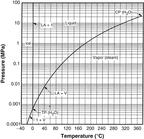
9.3.1. Water
Figure 9.1 shows the P-T diagram for water. This plot is to scale and shows the vapor pressure, melting curve, and sublimation curve.
As was discussed earlier, note how the three loci intersect in a triple point. Also, note how the three two-phase loci map out the single-phase regions. For example, the single-phase vapor region is bounded by the vapor + liquid locus and the vapor + solid locus.
Similar diagrams could have been constructed for the other components commonly found in natural gas.
9.4. Binary Systems
By adding a second component, we have added a degree of freedom. In Eqn (9.1) when N is increased by one, then the degree of freedom, F, is increased by one as well.
The P-T plane becomes a prism with composition being the third dimension. Two of the faces of the prism represent the pure components and are the P-T diagrams discussed earlier. Because it is difficult to interpret, the prism is often projected onto the P-T plane. In this manner, a binary P-T diagram is constructed.
A binary system existing in two-phases occupies a region in the P-T plane, as opposed to a curve for a pure component. On the other hand, for three-phase equilibrium, which is triple points for a one-component system, there are curves in the P-T plane for a binary system.
To construct a P-x diagram from the P-T diagram, the temperature is fixed and a plane is cut through the P-T projection. Similarly, for the T-x diagram the pressure is fixed.
4. The two-phase equilibrium for a pure component intersects the pure component axes on the P-x and T-x diagrams.
For example, the vapor pressure is a single point on the pure component axis. If, for a given temperature or pressure, both of the vapor pressures exist, then both occur on the P-x or T-x diagram.
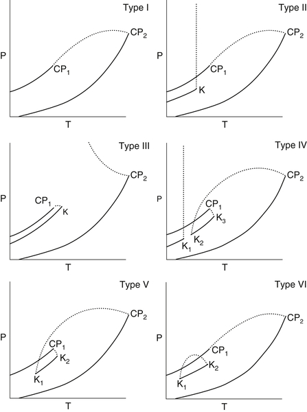
5. Binary critical loci extend from the pure component critical point. The critical locus does not always extend continuously between the two pure component critical points. Critical loci exist that do not end at a pure critical point.
In a classic paper in the area of fluid phase equilibria, Scott and Van Konynenburg (1970) showed that there are six basic types of binary fluid phase equilibria based on the possible binary critical loci. These are shown in Fig. 9.2. One problem with this is that solid phases can interfere with the predicted fluid phase behavior. For example, it is difficult to categorize the system water + methane into this scheme because an aqueous liquid phase cannot exist at the temperatures required for a liquid methane-rich phase to form.
6. Three-phase surfaces are curves when projected into the P-T plane. That is, the compositional effect is apparently removed.
7. Pure component triple points are the endpoints from one of the many binary three-phase loci.
The phase rule indicates that it is impossible for a pure component to simultaneously exist in four phases. This is not the case with a binary mixture. From the phase rule, for two components and four phases, there is zero degree of freedom. Thus, a point where four phases are in equilibrium, called a quadruple point, is a single point when projected into the P-T plane.
8. Quadruple points occur at the intersection of four three-phase loci.
The next rules are useful for constructing P-x and T-x diagrams.
9. The two single-phase regions adjacent to a two-phase region must be the two phases that correspond to the two-phase region. For example, a vapor–liquid region is adjacent to a liquid region and a vapor region.
10. A three-phase point on a P-x or T-x diagram is a horizontal line. The two endpoints and a central point are the compositions of the three phases.
11. The three regions that connect to the three-phase line on a P-x or T-x diagram are two-phase regions, which make up the three-phase line. For example, a three-phase solid-liquid-vapor line is connected to three two-phase regions: vapor–liquid, vapor–solid, and solid–liquid.
A useful tool in the construction of these phase diagrams is the ability to calculate the water content of a gas. Several methods are presented in the next chapter for performing such calculations.
9.4.1. Constructing T-x and P-x Diagrams
The construction of either a T-x or a P-x diagram usually begins with a P-T diagram, or at least it requires knowledge of the various pure component two-phase loci and the binary three-phase loci. This information is best extracted from the P-T diagram.
The first step is to draw a line on the P-T diagram corresponding to the pressure of interest (for a T-x diagram) or the temperature of interest for a P-x diagram. For example, to construct a P-x diagram at 10 °C, draw the line at t = 10 °C. Determine which loci are intersected by this isotherm.
Plot the pure component two-phase points on the appropriate axis. Plot the horizontal line that corresponds to the various three-phase loci. The ends of this horizontal line correspond to the composition of two of the coexisting phases. The composition of the third phase is intermediate of these two compositions. That is, it lies on the line somewhere between the endpoints.
Use the rules presented earlier to join the points and lines to construct the various two-phase and single-phase regions. This quick construction results in a schematic P-x diagram, which, if carefully used, is sufficient for most applications. Phase equilibrium calculations are required in order to include the precise compositions of the various phases. Then these must be plotted to scale.
9.4.2. Methane + Water
Ironically, one system that does not fall into the classification of Scott and Van Konynenburg (1970) is methane + water. Because the critical point of methane is at such a low temperature, a methane-rich liquid cannot form in the presence of liquid water. The P-T diagram for this system is shown in Fig. 9.3. The vapor pressure curve of methane is at such a low temperature that it is not included.
From the P-T diagram, and some additional information regarding composition (given in a previous chapter), a P-x diagram at 10 °C (50 °F) can be constructed. As noted earlier, at 10 °C, methane does not liquefy and, thus, none of the loci intersects the pure methane axis. That is, there is no possibility of equilibria between two phases composed of pure methane. On the other hand, the vapor pressure of water at 10 °C is 1.23 kPa (0.18 psia).

In this and subsequent discussion, the reader is cautioned about kPa and MPa. The various pressures differ by orders of magnitude and the switch between kilo and mega makes the numbers more rational.
In addition, from information presented earlier, the hydrate pressure at this temperature is 7.25 MPa. From this information and the rules presented earlier, the diagram in Fig. 9.4 was constructed. Please note that this plot is not to scale, although several pressure and compositions are noted.
At the three-phase point (hydrate + vapor + aqueous liquid), the vapor is essentially pure methane and the aqueous phase is nearly pure water. The compositions of these phases are given in Table 2.2.
From the phase diagram, we can make a few observations. Consider an equimolar mixture of methane and water at 10 °C and 10 MPa (50 °F and 1450 psia). According to the phase diagram, this mixture exists in two phases: (1) a hydrate and (2) a vapor. In other words, a hydrate exists without free-water being present.
Next, consider a mixture that is very lean in methane, for example 0.1 mol%. At this concentration, there is not enough methane present to form a hydrate. All of the methane remains in an aqueous solution, regardless of the pressure.
Figure 9.4(a) is a magnification of a region of Fig. 9.4, but it is a mirror image and it is to scale so that qualitative analysis can be made based on this chart. The aqueous dew point portion of the curve is the prediction from AQUAlibrium and the water content in the hydrate region is an extrapolation, based on information presented in the next chapter.

Consider a mixture containing 400 ppm of water. From Fig. 9.4(a), this mixture has a water dew point of about 3800 kPa (550 psia). A hydrate will form once the pressure reaches 7250 kPa (1050 psia). At this point, the gas in equilibrium with the hydrate is estimated to be 245 ppm water. Therefore, any mixture of methane + water less than 245 ppm water will have a hydrate pressure greater than 7250 kPa (1050 psia). For example, a mixture containing 215 ppm water would not form a hydrate until 9000 kPa (1300 psia).
9.4.3. Free-Water
Figure 9.4, the P-x diagram for methane + water, demonstrates the so-called “phase diagram argument” against the need for free-water to be present in order to form a hydrate. For example, for an equimolar mixture of methane + water at 10 °C and 10 MPa, what phases exist? From the phase diagram, there is only hydrate and vapor – where is the free-water? This demonstrates clearly that it is not necessary to have free-water in order to have a hydrate.
The “frost argument” against the need for free-water was presented at the end of Chapter 1. However, we can revisit the frost argument using the phase diagram. This was demonstrated earlier with the mixture of methane + water with a water content of 215 ppm. When this mixture is compressed, an aqueous phase (i.e., free-water) is not encountered. The hydrate sublimes directly out of the gas phase, just like frost from the air.
9.4.4. Carbon Dioxide + Water
The P-T diagram for the system carbon dioxide + water is shown in Fig. 9.5. A quick comparison of Figs 9.3 and 9.5 shows that the carbon dioxide + water are significantly more complicated than that for methane + water.
In this case, a second liquid, rich in carbon dioxide, can form. Note the three-phase locus, LA + LC + V, ends in a three-phase critical point, K. At this point, the properties of the vapor and the CO2-rich liquid become the same. A small critical locus extends from the K point to the critical point of pure CO2.

The reader will also notice some loci on this diagram that have not been discussed up to this point. In particular, are the LC + H + V loci. This curve is almost coincident with the vapor pressure of pure CO2.
The phase diagrams for ethane, propane, isobutane, and hydrogen sulfide with water are similar to carbon dioxide + water.
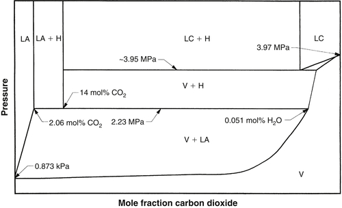
The P-x diagrams for the binary mixture carbon dioxide + water are also considerably more complicated than those for methane + water. As a first example, consider the P-x diagram at 5 °C, which is presented as Fig. 9.6. At this temperature, the vapor pressure of water is 0.873 kPa and that of CO2 is 3.97 MPa. Interpolating Table 2.7 gives the pressure for the LA + H + V locus as 2.23 MPa. From the previous discussion, the LC + H + V locus is assumed to be at a pressure slightly less than the vapor pressure. The compositions noted on this plot are also from Table 2.7.
Next, consider the P-x diagram at 11.3 °C. At this temperature, the vapor pressure of water is 1.34 kPa and CO2 is 4.65 MPa. At this temperature, the LA + LC + V and LC + LA + H loci are also crossed. The pressure and composition for the LC + LA + H were taken from Table 2.7. The pressure at this point is 20.0 MPa. The pressure and compositions along the LA + LC + V were calculated using AQUAlibrium. This information was used to construct the P-x diagram shown in Fig. 9.6.

9.4.5. Hydrogen Sulfide + Water
A detailed description of the phase diagrams for the binary system hydrogen sulfide + water was presented in the papers by Carroll (1998a,b). The phase equilibria in this system are analogous to those for water + carbon dioxide.
9.4.6. Propane + Water
A detailed review of the phase diagrams for the binary system propane + water was described in the paper by Harmens and Sloan (1990).
9.5. Phase Behavior below 0 °C
It is an interesting question to ask which solid phase will form at temperatures below 0 °C – ice or hydrate? To address this question, we examine the low temperature phase diagrams.
At this point, it is worth repeating that a discussion of water content of gases, including temperatures below 0 °C, is included in the next chapter.
9.5.1. Methane + Water
First, consider the binary mixture methane + water and construct a P-x diagram at −10 °C. From Fig. 9.3, we can see that two loci are crossed: (1) the sublimation curve for pure water (I + V) at 0.206 kPa and (2) a binary three-phase locus (H + I + V) at about 2 MPa. Fig. 9.7 shows the P-x diagram at this temperature.

If you compress a mixture containing 10% methane from a low pressure, the frost point is reached at about 0.23 kPa. The frost point is where the first crystal of solid forms from a gas mixture. This solid is ice and contains no methane. As the compression continues, more ice is formed and the water from the mixture is consumed. The resultant vapor is richer in methane.
At a pressure of 1.827 MPa, the first crystal of hydrate forms. At this point, three phases are in equilibrium: ice (solid water), hydrate (containing about 14% methane and 86% water), and vapor (about 99.99% methane and a little bit more than 0.01% water (about 0.092 mg/Sm3 or 5.7 lb/MMCF)).
As we continue to compress the mixture, more hydrate is formed and the vapor disappears. Finally, all of the vapor disappears and we enter a region where two solids are in equilibrium: ice and hydrate.
Next, consider a mixture that contains 24% methane. Again, at low pressure, the entire mixture is a gas. Once the mixture is compressed to about 0.275 kPa, the frost point is reached. Again, this solid is pure ice.
Upon further compression, this mixture behaves in a manner similar to the previous mixture – more solid is formed and vapor is consumed.
Again, like the previous mixture, at 1.827 MPa, a three-phase point is reached and hydrate begins to form. However, unlike the previous mixture, further compression results in the ice phase disappearing rather than the vapor. Finally, a point is reached where all of the ice is consumed and only hydrate and vapor remain.
As a final scenario, consider a mixture that is very rich in methane, say 99.999% (which is equivalent to 0.0076 mg/Sm3 or 0.47 lb/MMSCF). With this mixture, the ice phase is never encountered. The first solid phase encountered is the hydrate. Because this mixture is lean in water, the hydrate is encountered at a pressure greater than the three-phase pressure.
Note that in none of these scenarios is liquid water ever encountered.
9.6. Multicomponent Systems
Beyond binary systems, the application of the rules becomes more difficult. With the addition of more components, the phase rule dictates that we now have more degrees of freedom.
With fluid phase equilibria, in multicomponent systems, the design engineer usually constructs a phase envelope, a map that shows the regions where the stream exists as a liquid, a vapor, or as two phases.
The construction of a phase envelope is virtually impossible without computer software. The number of calculations and the complexity of the calculations make hand calculations virtually impossible. Typically, the design engineer can handle perhaps one or two such hand calculations, but beyond that…
9.6.1. An Acid Gas Mixture
As an example of a phase diagram for a multicomponent mixture, consider an acid gas with the following composition (on a water-free basis):
| Hydrogen Sulfide | 47.20 |
| Carbon dioxide | 49.10 |
| Methane | 3.19 |
| Ethane | 0.51 |

Furthermore, the mixture is 90 mol% acid gas and 10 mol% water.
Figure 9.8 shows the P-T phase diagram for this system. The banana-shaped region is what is usually thought of as the “phase envelope.” These are the nonaqueous phase dew- and bubble-points and they intersect at a multicomponent critical point.
The hydrate locus is also plotted on this figure. Along the hydrate locus, various phase combinations are encountered. At low pressure, the equilibrium is LA + V + H. In this case, the hydrate locus intersects the phase envelope. As it traverses the phase envelope, there are four phases in equilibrium LA + LH + V + H, where LH is used to designate the nonaqueous liquid phase. Note that this is a quadruple locus.
For systems containing more than two components, there can be a quadruple locus because we have additional degrees of freedom. Once the hydrate locus exits the phase envelope there is no more vapor and the equilibrium is LA + LH + H.
Finally, the curve near the bottom of the plot is the aqueous phase dew point locus. At pressures greater than this locus, an aqueous phase forms. It is not unusual to omit this locus because it is usually at very low pressure.
9.6.2. A Typical Natural Gas1
Consider a natural gas with a composition (on a water-free basis) as follows:
| Methane | 70.85 mol% |
| Ethane | 11.34 |
| Propane | 6.99 |
| Isobutane | 3.56 |
| n-butane | 4.39 |
| Carbon dioxide | 2.87 |
Figure 9.9 shows the P-T diagram for such a system. The aqueous dew point locus has been omitted on this plot, but the reader should be aware of its existence.
The most obvious difference between this phase diagram and that presented previously for the acid gas is the large retrograde region.
Also shown on this plot is the hydrate locus. Compression from low pressure enables the hydrate locus to intersect the phase envelope and a second liquid begins to form. As the pressure raises, more of the second liquid forms as expected, but a point is reached where the amount of the second liquid reaches a maximum. Beyond that point, the amount of the second liquid decreases until none remains – a retrograde dew point.

Examples
Example 9.1
Calculate the degrees of freedom for a single component system existing in four phases at equilibrium.
Answer: From the phase rule, we have N = 1 and p = 4. Thus:

This is an impossible situation – you cannot have a negative number of degrees of freedom. Therefore, a single component cannot exist in four equilibrium phases.
Example 9.2
Calculate the degrees of freedom for a two-component system existing in four phases at equilibrium.
Answer: From the phase rule, we have N = 2 and p = 4. Thus:

Zero degrees of freedom correspond to a fixed point in the P-T plane and is the quadruple point discussed earlier. Although a single component cannot exist in four phases, a two-component system can.
Example 9.3
At 15 °C and 30 MPa and a composition of 10% water and 90% methane (molar basis), what phases are present? Construct a phase diagram using the information provided in Chapter 2, to answer this question.
Answer: The construction of the phase diagram is left to the reader, but it will be similar to Fig. 9.4.
For the remainder of the question, from Table 2.2, the hydrate formation pressure for methane at 15 °C is 12.79 MPa. Therefore, at 30 MPa, a hydrate will form. Based on the overall composition of the mixture, the phases in equilibrium will be a vapor and a hydrate.
Example 9.4
At 10 °C, methane forms a hydrate at 7.25 MPa. How dry does methane have to be before a hydrate will form at a higher pressure at 10 °C? Use the information in Table 2.2 to answer this question. Express the results in ppm and in lb/MMCF.
Answer: From Table 2.2 the water content of the vapor in equilibrium with the hydrate is 0.025 mol%. Therefore, the gas must contain less than this amount of water.
Converting to ppm:
![]()
Converting to lb/MMCF (assuming standard conditions are 60 °F and 14.696 psi). The volume of 1 lb/mol of gas is:
![]()
Then converting from mole fraction to lb/MMCF gives

Therefore, the gas will not form a hydrate if the water content is less than about 12 lb of water per million standard cubic feet of gas.
Example 9.5
A gas mixture made up of 0.01 mol% water (100 ppm) and the balance is methane. What is the water dew point pressure for this gas at 10 °C?
Answer: From Fig. 9.4, we can see that at these conditions the gas does not have a water dew point. For a mixture with this composition, at pressures below 44.1 MPa, an aqueous phase does not form. At pressures greater than 44.1 MPa, a hydrate may form, depending upon the slope of the boundary of the V + H region. However, an aqueous phase will never form.
The term “water dew point” is commonly encountered in the natural gas business. The term is used to describe the water content of a gas, even though that gas may not have a true water dew point, as was shown in this example.
Example 9.6
A gas mixture made up of 0.01 mol% water and the balance is carbon dioxide. What is the water dew point pressure for this gas at 5 °C?
Answer: This is similar to the previous example, but the phase behavior is different.
From Fig. 9.10, it can be seen that a mixture this lean in water does not have a water dew point. At pressures below about 3.95 MPa, the mixture is always a gas. Eventually, a point is reached where a liquid begins to condense, but this liquid is a carbon dioxide-rich liquid (LC) and not an aqueous liquid. At higher pressures, the mixture becomes completely liquefied. The small amount of water will remain in solution and an aqueous phase will never form.
Example 9.7
An equimolar mixture of methane and water is compressed at 10 °C from a very low pressure to a very high pressure. What phases will be encountered during this compression?
Answer: We will conduct this “thought” experiment in an imaginary cylinder-piston arrangement. The piston must be of immense size in order to conduct the actual experiment, so it is possible, but impractical.
To begin, at very low pressure the mixture is a gas.
From Fig. 9.4, as the gas is compressed, the first region entered is the V + LA. That is how we reach an aqueous phase dew point. From AQUAlibrium, this dew point is estimated to be at 2.45 kPa.
Additional compression takes us further into the V + LA region. Once we reach a pressure of 7.25 MPa, the hydrate starts to form. Continued compression (i.e., reduction in volume) results in an increase in the amount of hydrate present and a reduction in the amount of aqueous liquid; however, the pressure remains unchanged. In addition, the compositions of the three phases are those given in Fig. 9.4 and remain unchanged during further compression.
Eventually, all of the aqueous liquid disappears and the V + H region is entered. For our purposes, we remain in the V + H region regardless of further compression. In reality, at very high pressures, other phases of solid water will be encountered.
Example 9.8
Return to Example 1.1 and we can now address the question of pressure and temperature. Will a hydrate form?
Answer: First, the VMGSim software was used to calculate the phase envelope for this mixture. The hydrate curve was estimated using: (1) VMGSim, (2) EQUI-PHASE Hydrate, and (3) CSMHYD. The three hydrate curves are plotted in Fig. 9.11. Finally, the operating conditions given are shown on the plot. The three hydrate predictions are in good agreement. The difference between the three of them is less than 1 °C on average from pressures up to 11 MPa.
From this plot, for this mixture, it is clear that pipeline conditions are in the region where a hydrate can be expected. The operating point lies to the left of the hydrate curve and, thus, is in the region where a hydrate can be expected.
3. The right combination of temperature and pressure:
However, there are some other interesting observations that can be made from this plot. Because the operating conditions are inside the phase envelope, the pipeline is operating in three phases: natural gas, condensate, and water, not just gas and water.

The critical point is not shown on this graph because it is at a temperature less than the scale of the graph. The critical point calculated by VMGSim is −53 °C and 7.64 MPa. The cricondentherm, the highest temperature at which two hydrocarbon phases can exist, is +29 °C and 4.76 MPa. The portion of the plot shown in Fig. 9.11 represents a portion of the retrograde region.
..................Content has been hidden....................
You can't read the all page of ebook, please click here login for view all page.