In contrast to the methods outlined in the previous chapter, the subject of this chapter is the rigorous thermodynamic models for predicting hydrates formation. Although the methods are complex and only provided in a rather cursory manner, these are the methods used in the computer software programs commonly used by engineers in the field. Several computer programs are used to show the accuracy of the predictions. The main focus of this chapter is to provide several examples that demonstrate the accuracy of the hydrate software packages available to process engineers.
Keywords
Free energy; Software
The emergence of powerful desktop computers has made the design engineer's life significantly easier. No longer do engineers have to rely on the approximate hand calculation methods, such as those provided earlier for hydrate formation estimates. In addition, a wider spectrum of additional calculations is available to them. This is true for hydrate calculations in which a number of software packages are available.
However, engineers should not blindly trust these programs—it is the responsibility of the user to ensure the software selected is appropriate for the job and gives accurate results.
The bases of these computer programs are the rigorous thermodynamic models found in the literature. Three of the more popular ones will be briefly reviewed here. This is followed by a brief discussion of the use of some of the available software packages.
As was mentioned previously, one of the problems in the study of gas hydrates was the observation that they were nonstoichiometric. First, scientists had to come to terms with this as an observation. Any model for hydrate formation had to handle this somewhat unusual property. Next, the fact that there is more than one type of hydrate had to be addressed. Rigorous models would have to distinguish between the various types of hydrates.
4.1. Phase Equilibrium
The criteria for phase equilibrium, established over 100years ago by Gibbs, are that: (1) the temperature and pressure of the phases are equal, (2) the chemical potentials of each of the components in each of the phases are equal, and (3) the global Gibbs free energy is a minimum. These criteria apply to phase equilibrium involving hydrates and form the basis for the models for performing hydrate equilibrium calculations.
Most phase equilibrium calculations switch from chemical potentials to fugacities, but hydrate calculations are usually performed based on chemical potentials. In the calculation of hydrates, the free energy minimization is also important. The stable hydrate phase (type I, II, or even H) is the one that results in a minimum in the Gibbs free energy. Therefore, simply meeting the first two criteria is not sufficient to solve the hydrate problem.
From a thermodynamic point of view, the hydrate formation process can be modeled as taking place in two steps. The first step is from pure water to an empty hydrate cage. This first step is hypothetical, but is useful for calculation purposes. The second step is the filling of the hydrate lattice. The process is as follows:
Pure water(α)→empty hydrate lattice(β)→filled hydrate lattice(H)
The change in chemical potential for this process is given as:
μH−μα=(μH−μβ)+(μβ−μα)
(4.1)
where μ is the chemical potential and the superscripts refer to the various phases. The first term after the equal sign represents the stabilization of the hydrate lattice. It is the variation in the models used to estimate this term that separates the various models.
The second term represents a phase change for the water and can be calculated by regular thermodynamic means. This term is evaluated as follows:
where R is the universal gas constant, T is the absolute temperature, P is the pressure, H is the enthalpy, v is the molar volume, the subscript O represents a reference state, and the Δ terms represent the change from a pure water phase (either liquid or ice) to a hydrate phase (either type I or II). The bar over the temperature in the last term in Eqn (4.2) indicates that this is an average temperature. The various properties required for this calculation have been tabulated and are available in the literature (see Pedersen et al., 1989 for example).
This term is virtually the same regardless of the model used. Subtle changes are made to account for other changes made to the model, but, theoretically, the same equation and set of parameters should apply regardless of the remainder of the model.
4.2. van der Waals and Platteeuw
The first model for calculating hydrate formation was that of van der Waals and Platteeuw (1959). They postulated a statistical model for hydrate formation. The concentration of the non-water species in the hydrate was treated in a manner similar to the adsorption of a gas into a solid. For a single guest molecule, this term is evaluated as follows:
μH−μβ=RT∑iνiln(1−Yi)
(4.3)
where νi is the number of cavities of type I and Y is a probability function. The Y is the probability that a cavity of type I is occupied by a guest molecule and is given by:
Yi=ciP1+ciP
(4.4)
The ci in this equation is a function of the guest molecule and the cage occupied and P is the pressure. Although it is not obvious from this discussion, the cis are also functions of the temperature.
A simple example—because ethane only occupies the small cages of a type I hydrate, then ci for ethane for the small cages is zero. On the other hand, methane, which is also a type I former, occupies both the large and small cages. Therefore, both the cis for this component are non-zero.
4.3. Parrish and Prausnitz
The approach of the original van der Waals and Platteeuw (1959) method provided a good basis for performing hydrate calculations, but it was not sufficiently accurate for engineering calculations. One of the first models with the rigor required for engineering calculations was that of Parrish and Prausnitz (1972).
where the second sum is over all components. The probability function for a component becomes:
YKi=ciPK1+∑jcijPj
(4.6)
Here, the summation is also over the number of components and the P followed by a subscript is the partial pressure for a given component. The other components are included in this term because they are competing to occupy the same cages. Thus, the presence of another guest molecule reduces the probability that a given guest can enter the hydrate lattice.
Second, Parrish and Prausnitz (1972) replaced the partial pressure in Eqn (4.6) with the fugacity. There is no simple definition for the thermodynamic concept of fugacity. Usual definitions given in thermodynamics textbooks rely on the chemical potential, which is an equally abstract quantity. For our purposes, we can consider the fugacity as a “corrected” pressure, which accounts for nonidealities. Substituting the fugacity into Eqn (4.6) results in:
YKi=cifˆI1+∑jcijfˆj
(4.7)
where fˆI is the fugacity of component I in the gaseous mixture. This allowed their model to account for nonidealities in the gas phase and thus to extend the model to higher pressures. In addition, some of the parameters in the model were adjusted to reflect the change from pressures to fugacities and to improve the overall fit of the model. That is, a different set of cis is required for the fugacity model than for the pressure model.
It is interesting to note that at the time that Parrish and Prausnitz (1972) first presented their model, the role of n-butane in hydrate formation was not fully understood. Although they give parameters for many components (including most of the components important to the natural gas industry), they did not give parameters for n-butane. Later modifications of the Parrish and Prausnitz method correctly included n-butane.
4.4. Ng and Robinson
The next major advance was the model of Ng and Robinson (1977). Their model could be used to calculate the hydrate formation in equilibria with a hydrocarbon liquid.
First, this required an evaluation of the change in enthalpy and change in volume in Eqn (4.2), or at least an equivalent version of this equation.
In the model of Ng and Robinson (1977), the fugacities were calculated using the equation of state of Peng and Robinson (1976). This equation of state is applicable to both gases and the non-aqueous liquid. Again, small adjustments were made to the parameters in the model to reflect the switch to the Peng–Robinson equation.
Similarly, the Soave (1972) or any other equation of state applicable to both the gas and liquid could be used. However, the Soave and Peng–Robinson equations (or modifications of them) have become the workhorses of this industry.
It is important to note that later versions of the Parrish and Prausnitz method were also designed to be applicable to systems containing liquid formers.
4.5. Calculations
Now that one has these equations, how does the calculation proceed? For now, we will only consider the conditions for incipient solid formation. For example, given the temperature, at what pressure will a hydrate form for a given mixture?
First, you perform the calculations assuming the type of hydrate formed. Use the equations outlined above to calculate the free energy change for this process. This is an iterative procedure that continues until the following is satisfied:
μH−μα=0
Remember, at equilibrium, the chemical potentials of the two phases must be equal. For a pure component in which the type of the hydrate is known, this is when the calculation ends (provided you selected the correct hydrate to begin with).
Next, repeat the calculation for the other type of hydrate at the given temperature and the pressure calculated above. If the result of this calculation is:
μH−μα>0
then the type of hydrate assumed initially is the stable hydrate and the calculation ends. If the difference in the chemical potentials is less than zero, then the hydrate type assumed to begin the calculation is unstable. Thus, the iterative procedure is repeated assuming the other type of hydrate. Once this is solved, the calculation is complete.
This represents only one type of calculation, but it is obvious from even this simple example that a computer is required.
4.5.1. Compositions
From the development of the model, as discussed above, it appears as though the bases for obtaining the model parameters are experimentally measured compositions. However, accurate and direct measurements of the composition are rare. The compositions are usually approximated from pressure–temperature data. In reality, the model parameters are obtained by fitting the pressure–temperature loci and deducing the compositions.
However, using this type of model allows us to estimate the composition of hydrates. Again, this may seem obvious, but the parameters were obtained by fitting pressure–temperature data and not by fitting composition data, which would seem more logical.
Figure 4.1 shows the ratio of water to hydrogen sulfide in the hydrate at a temperature of 0°C. The ratio is always greater than the theoretical limit 5¾ (see Chapter 2). Because this ratio is always greater than the theoretical limit, this means that there are more water molecules per H2S molecules than the value that results if all of the cages are occupied. Physically, this translates to there being unoccupied cages.
At approximately 1MPa, the hydrogen sulfide liquefies and the equilibrium changes from one between a liquid, a vapor, and a hydrate to two liquids and a hydrate.
Figure 4.1The Ratio of Water to Hydrogen Sulfide in the Hydrate at 0°C.
4.6. Commercial Software Packages
There are several software packages available that are dedicated to hydrate calculations. These include EQUI-PHASE Hydrate from Schlumberger in Canada, PVTSim from Calsep in Denmark, and Multiflash from Infochem (now KBC Advanced Technologies) in the United Kingdom. In addition, the packages CSMHYD and CSMGEM are available from the Colorado School of Mines in Golden, Colorado. Unlike most commercial hydrate software, a thorough description of CSMGEM is available in the literature (Ballard and Sloan, 2004).
Most of the popular, general-purpose process simulation programs include the capability to predict hydrate formation. Often, this includes warnings about streams where hydrate formation is possible. These include Promax (Prosim is a previous generation process simulator) from Bryan Research & Engineering (Bryan, TX), Hysys and Aspen from Aspen Technology (Cambridge, MA), VMGSim from Virtual Materials Group (Calgary, Canada), and others.
4.7. The Accuracy of These Programs
Earlier, we compared the hand calculations against two models. We shall do the same here. The software programs examined will be: (1) CSMHYD (released August 5, 1996), (2) EQUI-PHASE Hydrate (v. 4.0), (3) Prosim (v. 98.2), and (4) Hysys (v. 3.2, Build 5029). Although these may not be the most recent versions of these software packages, the results obtained are still typical of what can be expected.
The comments presented in this section should not be interpreted as either an endorsement or as a criticism of the software. The predictions are presented and the potential ramifications are discussed. If the reader has access to a different software package, they are invited to make these comparisons for themselves. All of the software packages have their strengths and their weaknesses. General conclusions based on a small set of data (or worse, no data!) are usually not warranted.
4.7.1. Pure Components
Perhaps the simplest test of a correlation is its ability to predict the pure component properties. One would expect that the developers of these software packages used the same data to generate their parameters as were used to generate the correlations. Large deviations from the pure component loci would raise some questions about the accuracy of the predictions for mixtures.
The following pure components will be discussed and several plots will be presented. The points on these plots are the same as those on Figs 3.4 and 3.5 and are from the correlations presented in Chapter 2. They are not experimental data and should not be interpreted as such. The curves on the plots are generated using the above-mentioned software packages.
One thing that should be kept in mind when reviewing the plots in this section is that predicting the hydrate temperature less than the actual temperature could lead to problems. Potentially, it means that you predict that hydrates will not form, but, in reality, they do.
4.7.1.1. Methane
Figure 4.2 shows the hydrate locus for pure methane. Throughout the range of pressure shown on this plot, all three software packages are of acceptable error. Only at extreme pressures do the errors exceed 2°C.
First, consider pressures below 10MPa (1450psia), which is a reasonable pressure limit for the transportation and processing of natural gas. However, it is not sufficient for the production of gas. The high-pressure region will be discussed later in this section.
Figure 4.2Hydrate Locus Loci of Methane.(Points from correlation.)
EQUI-PHASE Hydrate is an accurate prediction of the correlation in the low-pressure region, with errors much less than 1°C. At the lowest pressures, CSMHYD is also a very good fit. However, as the pressure increases, the deviations become larger. Once the pressure reaches 10MPa the CSMHYD predicts hydrate temperatures that are about 1°C too high. Throughout this region, Prosim consistently underpredicts the hydrate temperature by about 1°C.
At pressures greater than 10MPa, none of the three software packages is highly accurate. EQUI-PHASE Hydrate predicts a hydrate temperature that is consistently less than the correlation. At extreme pressures, the error is as much as 1°C. On the other hand, both Prosim and CSMHYD predict that the hydrate forms at higher temperatures than the correlation. At very high pressure, the errors from Prosim become quite large. For example, at 50MPa (7250psia), the difference is larger than 2°C. With CSMHYD, for pressure up to 50MPa, the errors are less than 2°C. However, as the pressure continues to increase, so does the observed error.
4.7.1.2. Ethane
Figure 4.3 shows the hydrate locus for pure ethane. It is clear from Fig. 4.3 that this locus is different from that of methane. First, ethane tends to form a hydrate at a lower pressure than methane. More significantly, at approximately 3MPa (435psia) the curves show a transition from the LA+H+V region (LA=aqueous liquid, H=hydrate, and V=vapor) to the LA+LH+H (LH=ethane-rich liquid). Therefore, we should examine the two regions separately. Experimental data for the ethane hydrate locus do not exist for pressure greater than about 20MPa, and, thus, the discussion is limited to this pressure.
EQUI-PHASE Hydrate almost exactly reproduces the LA+H+V locus from the correlation. CSMHYD overpredicts the hydrate temperature, but only slightly. Errors are less than one-half of a Celsius degree. On the other hand, Prosim underpredicts the hydrate temperature, but, again, the error is very small, and also are less than one-half of a Celsius degree.
Errors are slightly larger for the region LA+LH+H. EQUI-PHASE Hydrate predicts that LA+LH+H locus is very steep, steeper than the correlation indicates. Thus, as the pressure increases, so do the errors from EQUI-PHASE Hydrate. At 20MPa, the error is about 3°C. Both Prosim and CSMHYD better reflect the curvature of the LA+LH+H shown by the correlation. The error from Prosim is less than 1°C for this region. CSMHYD is slightly poorer with errors slightly larger than 1°C.
Figure 4.3Hydrate Loci of Ethane.(Points from correlation.)
4.7.1.3. Carbon Dioxide
Figure 4.4 shows the hydrate locus for carbon dioxide. The hydrate curve for CO2 is similar to that for ethane. As with ethane, we will examine two regions: (1) the LA+H+V, pressures less than about 4.2MPa (610psia), and (2) LA+LC+H (LC=CO2-rich liquid) for pressures greater than 4.2MPa.
For the LA+H+V region, both EQUI-PHASE Hydrate and CSMHYD accurately reproduce the correlation values. For these two packages, the errors are a small fraction of a Celsius degree. Prosim consistently underpredicts the hydrate temperature. The average deviation is about 1°C.
In the LA+LC+H region, all three packages are good predictions of the correlation data. However, in each case, the software packages overpredict the hydrate temperature. EQUI-PHASE Hydrate predicts the correlation data to better than one half of a Celsius degree. The other two packages have a maximum error of about 1°C.
Figure 4.4Hydrate Loci for Carbon Dioxide.(Points from correlation.)
4.7.1.4. Hydrogen Sulfide
The last of the pure components examined in this chapter will be hydrogen sulfide. Figure 4.5 presents the hydrate locus for H2S. Again, this is similar to those for ethane and CO2 inasmuch as they show the two regions: LA+H+V and LA+LS+H (LS is the hydrogen sulfide-rich liquid phase). As has been stated earlier, one of the important things about hydrogen sulfide is that it forms a hydrate at such low pressure and extends to high pressure.
In the LA+H+V region, both EQUI-PHASE Hydrate and CSMHYD accurately predict the hydrate formation region. The errors are less than 1°C and, in the case of EQUI-PHASE Hydrate, they are much less. Prosim consistently predicts a lower hydrate temperature than the correlation data. The errors are slightly larger than 1°C.
For the LA+LS+H region, both EQUI-PHASE Hydrate and CSMHYD accurately reproduce the correlation data. Again, Prosim underpredicts the hydrate formation temperature, typically by about 2°C.
Figure 4.5Hydrate Loci for Hydrogen Sulfide.(Points from correlation.)
4.7.2. Mixtures
In the previous chapter, several mixtures were examined. These same mixtures will be used here. The reader should cross-reference this section with the equivalent section in the previous chapter.
4.7.2.1. Data of Mei et al
The data of Mei et al. (1998) were used in the previous chapter for comparison with the hand calculation methods. Figure 4.6 shows the data for Mei et al. (1998) and the prediction from the three software packages.
All three of the software packages predict that the hydrate formation temperature is less than the experimental data. The maximum error for the EQUI-PHASE Hydrate is slightly less than 1.8°C. CSMHYD has a maximum error slightly larger than 2.1°C and, finally, Prosim has a maximum error slightly larger than 3.0°C.
Again, it is surprising that the errors from the models are as large as they are considering that the system is a very simple mixture. In fact, the K-factor method presented in Chapter 3, which is claimed to be simple and known to be not highly accurate, is as good as or better than the software packages.
Figure 4.6Hydrate Locus for a Synthetic Natural Gas Mixture (CH4 97.25mol%, C2H6 1.42%, C3H8 1.08%, i-C4H10 0.25%).
4.7.2.2. Data of Fan and Guo
The data of Fan and Guo (1999) for two mixtures rich in carbon dioxide were introduced in the previous chapter.
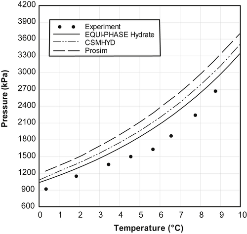
Figure 4.7 shows the experimental data for the mixture of CO2 (96.52mol%) and methane (3.48%) and the predictions from the three software packages.
At low pressures (less than about 3000kPa), all the models predict that the hydrate temperature is less that the experimental data. However, the difference is less than 1°C for CSMHYD and EQUI-PHASE Hydrate and slightly more for Prosim. For the single point at higher pressure (approximately 5000kPa), all three models predict a higher hydrate temperature than the experimental data.
Figure 4.8 shows the hydrate loci for the second mixture from Fan and Guo (1999). For the range of temperature shown, both CSMHYD and EQUI-PHASE Hydrate are excellent predictions of the data. However, EQUI-PHASE Hydrate had some trouble with this mixture. It was unable to calculate the hydrate locus over the entire range of temperature. Furthermore, it was unable to perform the point-by-point calculations for this mixture. Prosim consistently predicts that the hydrate temperature is lower that the experimental data. Typically, the errors are less than 1°C.
Figure 4.7Hydrate Locus for a Mixture of Carbon Dioxide (96.52mol%) and Methane (3.48mol%).
Figure 4.8Hydrate Locus for a Quaternary Mixture 88.53mol% CO2, 6.83% CH4, 0.38% C2H6, and 4.26% N2.
4.7.2.3. Data of Ng and Robinson
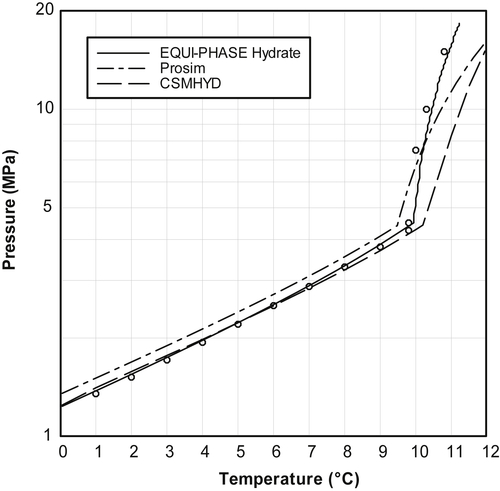
An important study is that of Ng and Robinson (1976, 1977). Because these data are so significant, it is highly likely that they were used in the development of the computer models. In the previous chapter, four mixtures of methane+n-butane were examined. Here, only a single mixture (CH4 [96.09mol%]+n-C4H10 [3.91%]) will be presented. The main reason for this is clarity. In addition, as was mentioned, these data were almost certainly used to develop the model parameters and, thus, it should come as no surprise that these models accurately predict these data.
Figure 4.9 shows the hydrate curves for this mixture. Both CSMHYD and EQUI-PHASE Hydrate are excellent predictions of the data with errors less than 1°C. Prosim consistently predicts that the hydrate temperature is less than the experimental data with errors larger than 2°C.
Also, note that these calculated loci do not show the unusual behavior that the K-factor method did (Fig. 3.13). This unusual behavior was an artifact of the K-factor method.
Figure 4.9Hydrate Loci for a Mixture of Methane and n-Butane.
4.7.2.4. Data of Wilcox et al
The data from Wilcox et al. (1941) were introduced in Chapter 3. These data are for sweet gas mixtures and the pressures range from 1.2 to 27.5MPa (175–3963psia), which corresponds to a temperature range of 3.6–25.2°C (38–77°F). There are three mixtures, therefore, the reader is referred to the previous chapter for more information about these mixtures.
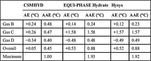
The data were compared to predictions from CSMHYD, EQUI-PHASE Hydrate, and Hysys. The table shows the average error (AE) in the predicted temperature (simply the sum of the differences between the predicted value and the experimental value) and the average absolute error (AAE), the average of the absolute value of the temperature differences. These values are summarized in Table 4.1. The upper part of the table is for Celsius temperatures and the lower for Fahrenheit.
For all three packages, the maximum error in the predicted hydrate temperature is less than 2°C (less than 3.5°F).
This is only one set of data and it is difficult to draw general conclusions, but, for this set of data, CSMHYD appears to be the best. For CSMHYD, the AE is only +0.1 and the AAE is 0.81, both in Celsius degrees.
4.7.3. Sour Gas
From Chapter 2, we can see that of the components commonly found in natural gas, hydrogen sulfide forms a hydrate at the lowest pressure and it persists to the highest temperatures. It was also shown that mixtures of hydrogen sulfide and propane exhibit hydrae azeoptropy, thus, sour gas mixtures, natural gas containing H2S, are an interesting class of mixtures.
Table 4.1
Comparison of Three Software Packages for Three Mixtures from Wilcox et al. (1941)
CSMHYD
EQUI-PHASE Hydrate
Hysys
AE (°C)
AAE (°C)
AE (°C)
AAE (°C)
AE (°C)
AAE (°C)
Gas B
+0.24
0.48
+0.14
0.24
+0.12
0.23
Gas C
+0.26
0.47
+1.58
1.58
+1.57
1.57
Gas D
−0.34
0.40
−0.48
0.48
−0.49
0.49
Overall
+0.05
0.45
+0.53
0.88
+0.52
0.88
Maximum
1.00
1.93
1.92
AE (°F)
AAE (°F)
AE (°F)
AAE (°F)
AE (°F)
AAE (°F)
Gas B
+0.43
0.86
+0.25
0.42
+0.21
0.42
Gas C
+0.46
0.84
+2.84
2.84
+2.83
2.83
Gas D
−0.61
0.72
−0.86
0.86
−0.89
0.89
Overall
+0.10
0.81
+0.96
1.58
+0.94
1.58
Maximum
1.80
3.47
3.45
AAE, average absolute error; AE, absolute error.
Carroll (2004) did a thorough study of the hydrate formation in sour gas mixtures. A review of the literature established a database of approximately 125 points. The database was made from three studies of sour gas mixtures: Noaker and Katz (1954), Robinson and Hutton (1967), and Sun et al. (2003). The maximum H2S concentration in the study of Noaker and Katz (1954) was 22mol%. In their study, the temperature ranged from 38 to 66°F (3.3–18.9°C) and the pressure from 150 to 985psia (1030–6800kPa). Robinson and Hutton (1967) studied hydrates in ternary mixtures of methane, hydrogen sulfide, and carbon dioxide over a wide range of pressures (up to 2300psia or 15,900kPa) and temperatures (up to 76°F or 24.4°C). The hydrogen sulfide content of the gases in the study of Robinson and Hutton (1967) ranged from 5% to 15% and the carbon dioxide from 12% to 22%. Sun et al. (2003) also measured the hydrate conditions for the ternary mixture of CH4, CO2, and H2S. This set covered a wide range of compositions (CO2 about 7mol% and H2S from 5 to 27mol%) for pressures up to 1260psia (8700kPa) and temperatures up to 80°F (26.7°C).
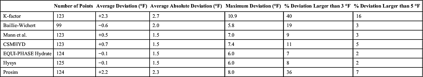
The AEs for both CSMHYD and EQUI-PHASE Hydrate are about 1.5°F (0.8°C). Typically, these methods are able to predict the hydrate temperature to within 3°F (1.7°C) 90% of the time. The hydrate prediction routine in Hysys, a general-purpose process simulator, was also quite accurate with an AE of 1.5°F (0.8°C). Hysys is able to predict the hydrate temperature to within 3°F (1.7°C) more than 90% of the time. On the other hand, Prosim, another general-purpose simulator program, was not as accurate. The AE for Prosim was about 2.3°F (1.3°C). It was able to predict the hydrate temperature to within 3°F (1.7°C) only about 65% of the time.
Although the averages noted above give an overall impression of the accuracy of these methods, the maximum errors reveal the potential for significantly larger errors. Even the computer methods have larger maximum errors, 6.0°F (3.3°C) for EQUI-PHASE Hydrate, 7.4°F (4.1°C) for CSMHYD, and 6.0°F (3.3°C) for Hysys, and 8.0°F (4.4°C) for Prosim.
Table 4.2 summarizes the results of this study, not only for the computer methods that are the subject of this chapter but also for some of the hand calculations presented in the previous chapter. The AE allows for positive errors and negative errors can cancel, whereas with the absolute value all errors are positive. The last two columns indicate the number of predictions with errors greater than 3 and 5°F. For example, CSMHYD predicts the experimental temperatures to within 3°F 89% of the time (11% have deviations greater than 3°F).
Table 4.2
Errors in Predicting the Hydrate Temperatures for Sour Gas Mixtures from the Overall Data Set
Number of Points
Average Deviation (°F)
Average Absolute Deviation (°F)
Maximum Deviation (°F)
% Deviation Larger than 3°F
% Deviation Larger than 5°F
K-factor
123
+2.3
2.7
10.9
40
16
Baillie-Wichert
99
−0.6
2.0
5.8
19
3
Mann et al.
123
+0.5
1.5
7.0
9
3
CSMHYD
123
+0.7
1.5
7.4
11
5
EQUI-PHASE Hydrate
124
−0.1
1.5
6.0
7
2
Hysys
125
−0.1
1.5
6.0
8
2
Prosim
124
+2.2
2.3
8.0
36
7
4.7.4. Third Party Studies
In his development of CSMGEM, Ballard (2002) did comparisons among the new software and four other software packages: CSMHYD, DBRHydrate (v. 5), Multiflash, and PVTsim. These results are repeated here without verification. The database that Ballard used consisted of more than 1500 data points. The purpose of this section is to present results that do not reflect any bias from this author.
The errors are the difference between the experimentally measured temperature and the predicted temperature for a given pressure for the specified mixture. These differences are averaged to get the values given in the tables that follow. Overall, the error for CSMGEM was 0.40°C and 0.66, 0.64, 0.54, and 0.54°C for CSMHYD, DBRHydrate, Multiflash, and PVTSim, respectively. These are equal to 0.72, 1.19, 1.15, 0.97, and 0.97°F for CSMGEM, CSMHYD, DBRHydrate, Multiflash, and PVTSim, respectively.
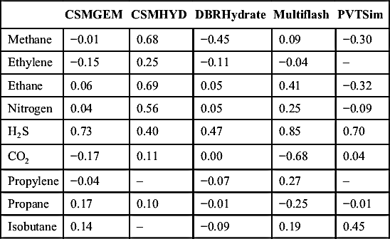
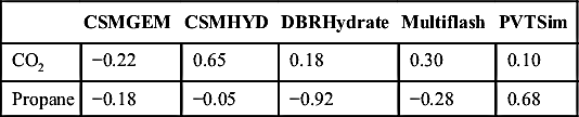
Table 4.3 gives the errors in the temperatures for nine pure components. Tables 4.4, 4.5, and 4.6 give the errors for binary mixtures with methane, ethane, and propane. Note these are AEs and, thus, negative values will cancel positive ones so, overall, the values look relatively small.
Table 4.3
Average Errors (Celsius Degrees) for the Hydrate Predictions from Five Software Packages for Pure Components
Although the Ballard (2002) study shows that CSMGEM is consistently more accurate than the other packages, it is probably fair to conclude that all give a prediction of acceptable accuracy.
4.8. Dehydration
One of the criteria for hydrate formation is that a sufficient amount of water be present. The hand calculations presented in Chapter 3 all assumed that plenty of water was present. The calculations presented from the software packages presented so far, also assume that plenty of water was present. For pure components, the minimum amount of water to be in the saturation region was given in Chapter 2.
Figure 4.10Hydrate Loci of Methane After Dehydration.
Methods for dehydration commonly used in the natural gas business are the topic of a subsequent chapter. In addition, further discussion of the water content of fluids in equilibrium with gases is presented later.
One of the advantages of a properly designed software package is that it can be used to predict the effect of dehydration on the hydrate formation conditions. Unfortunately, there is not a lot of experimental data available in the literature for building these models. More discussion of water content is given in Chapter 10 and the reader is referred to that chapter for more details.
Figure 4.10 shows some calculations for the effect of water content on the hydrate formation conditions. These calculations were performed using Prosim. The solid line on this plot labeled “saturation” is where plenty of water is present. This is the same curve as was plotted in Fig. 4.2. The other two plots on this figure are for a water content of 115mg/Sm3 (151ppm or 7lb/MMSCF) and the other is for 65mg/Sm3 (85.5ppm or 4lb/MMSCF).
Finally, it is probably fair to anticipate that the errors in the predictions shown on this plot are about ±2°C. This is based on the results for the systems presented earlier in this chapter.
The focus of Chapter 10 is the water content of natural gas but in equilibrium with liquid water and with solid phases. More details are presented in that chapter on the effect of water content.
4.9. Margin of Error
One of the purposes of this chapter was to demonstrate that the software methods are not perfect. They are, however, very good. However, the design engineer should always build in a margin of error into the process designs. It is typical to have a safety factor of at least 3°C (5°F). That is, if you calculate a hydrate formation temperature of 10°C, you should design to operate at 13°C or more.
Examples
Example 4.1
Methane forms a type I hydrate at 0°C and 2.60MPa (see Table 2.2). Given that csmall=3.049/MPa and clarge=13.941/MPa, calculate the saturation of the two cages for the methane hydrate using these values.
Therefore, at 0°C and 2.60MPa, the small cages are just less than 90% filled and the large cages are slightly more than 97% filled.
Note, a Windows Excel spreadsheet is provided to perform such calculations. In addition, for higher accuracy, the fugacity should be used in place of the pressure.
Example 4.2
What would the cs in Eqn (4.4) be for propane in a type I hydrate?
Answer: To begin with, propane forms a type II hydrate. Furthermore, propane will never enter the cages of a type I hydrate. Therefore, the cs for propane in a type I hydrate are zero.
This may seem obvious, but it is not. For example, nitrogen also forms a type II hydrate. However, in the presence of a type I hydrate former, nitrogen can enter the type I lattice. Therefore, the cs for nitrogen in a type I hydrate are non-zero.

 (4.2)
(4.2) (4.5)
(4.5) (4.6)
(4.6) (4.7)
(4.7)