Search in book...
Toggle Font Controls
Create new playlist

Name your new playlist

Playlist description (optional)
Sign In

Email address

Password

Forgot Password?

or

Continue with Facebook

Continue with Google
Sign Up

Full Name

Email address

Confirm Email Address

Password

or

Continue with Facebook

Continue with Google

Chapter 7

Combating Hydrates Using Heat and Pressure

Abstract

One of the criteria for hydrate formation is the right combination of temperature and pressure, with hydrate formation being favored by relatively high pressure and low temperature. Therefore, if the system is kept warm or at low pressure, hydrate formation can be avoided. Alternatively, if the temperature of the system is increased or the pressure is reduced, a hydrate plug can be melted. This chapter deals with combating hydrates with the use of heat, or more precisely high temperature and reducing the pressure. The major subtheme is the plugging of pipelines from hydrate formation. The mechanism for plug formation is examined briefly. The problem of melting hydrate plugs is reviewed and in particular the problems that may be encountered if the hydrate is not properly dealt with are discussed.

Keywords

Depressurizing; Hydrate plugs; Line heaters; Pipeline temperature loss

Much effort was expended in the earlier chapters of this book providing methods for determining the conditions of pressure and temperature at which hydrates would form for natural gas mixtures. Another means of combating hydrate formation is to avoid the regions of pressure and temperature where hydrates would form. This is the topic of this chapter.

The reason why a plug forms in a pipeline is because the three criteria for hydrate formation, given in Chapter 1, are present. There is water, gas, and the right combination of temperature and pressure. In this chapter, we are going to examine how we can take advantage of the third criteria in the battle against hydrates.

7.1. Plugs

Perhaps the most significant problem with hydrates is the plugging of pipelines, and much of the focus of this chapter is on pipelines. The hydrates really become problematic when they block or severally restrict the flow in a pipeline. Often hydrates form but flow with the fluid in the line causing only minimal flow problems.

It is worth noting that hydrate plugs tend to be porous and permeable, especially in condensate lines (Austvik et al., 2000). However, this is not always true and should not be assumed a priori.

Another important consideration is that one should not assume that there is only a single hydrate plug blocking the line. One should prepare for the possibility of multiple plugs blocking the flow line.

When it comes to melting hydrate plugs, patience truly is a virtue. It may take several days to melt a large plug. In addition, the application of a remedial measure usually will not result in an immediate observable change in the situation.

7.1.2. Plug Formation

For pipe flow, the hydrates initially are as for small particles. As mentioned in Chapter 1, these particles are formed at a nucleation site. The particles accumulate and may eventually form a flow blocking plug.

Typically, the outset of hydrate plugging is associated with an increase in pressure drop. This initial accumulation is called bedding and the pressure drop associated with bedding is due to restriction in flow. The nature of bedding is a function of many variables, including the velocity and the water cut. At high velocity, the hydrate particles are carried with the flow and thus there is less tendency to bed.

The pressure drop is erratic because the bedding is not yet a plug and quickly changes in size. As the hydrate accumulates into a plug, the pressure drop can increase dramatically. Eventually the hydrate accumulates into a flow blocking plug.

Another reason for the changes in pressure drop in hydrates systems is due to changes in viscosity. The formation of hydrate in a flow system will tend to increase the effective viscosity of the liquid phase, which in turn will increase the pressure drop.

Operators who observe these changes in the flow can assume that a flow blocking plug is inevitable and should try to take remedial action before the flow stops. This may include increasing the rate at which inhibitor is being injected or the use of some of the concepts presented in this chapter.

This description of the formation of hydrate plugs in pipe flow is based on research conducted at the Center for Hydrate Research at the Colorado School of Mines in Golden, Colorado.

7.2. The Use of Heat

We have already discussed the range of temperature and pressure where hydrates may form. To prevent the formation of hydrates, one merely has to keep the fluid warmer than the hydrate-forming conditions (with the inclusion of a suitable margin for safety). Alternatively, it may be possible to operate at a pressure less than the hydrate formation pressure.

With a buried pipeline, which loses heat to the surroundings as the fluid flows, the temperature must be such so that no point in the pipeline is in the region where a hydrate will form. This heating is usually accomplished by two means, either by using line heaters or heat tracing.

A heater can be used to warm the fluid. Because this is a single-point injection of energy, the amount of energy must be such that the fluid remains above the hydrate point until the next point where heat is added is reached. This means that the fluid entering the pipeline must be well above the hydrate temperature.

Another method to add heat to a system is to use heat tracing. In this method, the heat is injected continuously along a line. Thus the fluid temperature does not need to be very high at any single point, but with the continuous injection of energy the temperature of the fluid needs to be only above the hydrate temperature and not warmer.

Heat tracing can be electrical or a fluid medium (hot oil or glycol, for example). In either case, the heat trace is placed adjacent to the line that is to be heated.

Heat tracing is especially useful on valves. Valves are notorious for freezing because of cooling from the Joule–Thomson effect.

Another important tool in the fight against hydrate formation is the use of insulation. An insulated pipeline will lose heat at a slower rate than an uninsulated one. This translates into a lower temperature requirement for the outlet of the heater and ultimately a lower heater duty. And a lower duty translates into lower operating costs. As a matter of fact, the proper use of insulation may, in some case, negate the requirement for a heater altogether.

7.2.1. Heat Loss from a Buried Pipeline

Heat loss from a buried pipeline can be estimated using the fundamental principles of heat transfer. You begin with the basic heat transfer equation:

$Q = U A Δ T_{lm}$ $Q = U A Δ T_{lm}$

(7.1)

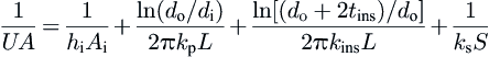
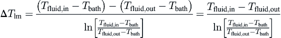
where Q is the heat transfer rate, U is the overall heat transfer coefficient, A is the area available for heat transfer, and ΔT_lm is the logarithmic mean temperature, which is difference given by:

$Δ T_{lm} = \frac{T_{fluid, in} - T_{fluid, out}}{\ln [\frac{T_{fluid, in} - T_{soil}}{T_{fluid, out} - T_{soil}}]}$ $Δ T_{lm} = \frac{T_{fluid, in} - T_{fluid, out}}{\ln [\frac{T_{fluid, in} - T_{soil}}{T_{fluid, out} - T_{soil}}]}$

(7.2)

where T is the temperature and the subscripts are sufficiently descriptive.

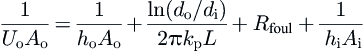
The overall heat transfer coefficient, U, is the sum of four terms: (1) convection from the fluid flowing in the line, (2) conduction through the pipe, (3) conduction through insulation (if present), and (4) resistance from the soil. The U is obtained from the following equation:

$\frac{1}{U A} = \frac{1}{h_{i} A_{i}} + \frac{\ln (d_{o} / d_{i})}{2 π k_{p} L} + \frac{\ln [(d_{o} + 2 t_{ins}) / d_{o}]}{2 π k_{ins} L} + \frac{1}{k_{s} S}$ $\frac{1}{U A} = \frac{1}{h_{i} A_{i}} + \frac{\ln (d_{o} / d_{i})}{2 π k_{p} L} + \frac{\ln [(d_{o} + 2 t_{ins}) / d_{o}]}{2 π k_{ins} L} + \frac{1}{k_{s} S}$

(7.3)

where h_i is the convective heat transfer coefficient for the fluid in the pipe, A_i is the inner surface area of the pipe, d_o and d_i are the outside and inside diameters of the pipe, k_p is the thermal conductivity of steel used to construct the pipe, L is the length of a pipe segment, t_ins is the thickness of the insulation, k_ins is the thermal conductivity of the insulation, k_s is the thermal conductivity of the soil, and S is the shape factor for the buried pipe.

7.2.1.1. Fluid Contribution

There are many correlations for estimating heat transfer coefficients. These are based on the properties of the fluid and flow considerations. However, almost all of them can be expressed in the dimensionless form:

$Nu = f (Re, \Pr)$ $Nu = f (Re, \Pr)$

(7.4)

where Nu is the Nusselt number, which is a dimensionless heat transfer coefficient; Re is the Reynolds number, which is a combination of the flow conditions and fluid properties and it is also dimensionless; and Pr is the Prandtl number, which is the dimensionless description of the fluid properties.

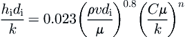
An example of such a correlation is the Dittus–Boelter equation (Holman, 1981):

$Nu = 0.023 {Re}^{0.8} \Pr^{n}$ $Nu = 0.023 {Re}^{0.8} \Pr^{n}$

(7.5)

where n = 0.4 for heating or n = 0.3 for cooling, which is the case for heat loss from a pipeline. Substituting the properties for the dimensionless groups yields:

$\frac{h_{i} d_{i}}{k} = 0.023 {(\frac{ρ v d_{i}}{μ})}^{0.8} {(\frac{C μ}{k})}^{n}$ $\frac{h_{i} d_{i}}{k} = 0.023 {(\frac{ρ v d_{i}}{μ})}^{0.8} {(\frac{C μ}{k})}^{n}$

(7.5a)

where ρ is the density of the fluid, v is the fluid velocity, μ is the viscosity of the fluid, C is the heat capacity of the fluid, and k is the thermal conductivity of the fluid (all other symbols were defined earlier). Rearranging this slightly yields:

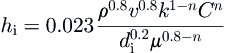$h_{i} = 0.023 \frac{ρ^{0.8} v^{0.8} k^{1 - n} C^{n}}{d_{i}^{0.2} μ^{0.8 - n}}$ $h_{i} = 0.023 \frac{ρ^{0.8} v^{0.8} k^{1 - n} C^{n}}{d_{i}^{0.2} μ^{0.8 - n}}$

(7.5b)

The Dittus–Boelter equation is limited to Reynolds numbers in the range 5000 < Re < 500,000 and for Prandtl numbers from 0.6 to 1000.

It is also worth noting that there are several other correlations available for estimating the heat transfer coefficient in tube flow. The reader should consult any textbook on the subject of heat transfer, such as Holman (1981), for more such correlations.

7.2.1.2. Pipe Contribution

The second term on the right hand side of Eqn (7.3) is the contribution from the conduction through the metal of the pipe.

Typically pipe comes in standard sizes that have descriptions via their nominal diameter in inches. Even in countries where the metric system of units is used, nominal pipe sizes are usually given in inches. For example, there is 3-in schedule 80 pipe, where the schedule number reflects the wall thickness of the pipe. Although this pipe is called 3-in, the outside diameter of the pipe is 3.500 in (88.90 mm) and the inside diameter is 2.900 in (73.66 mm). The physical sizes of standard pipe are readily available.

The thermal conductivity of carbon steel is about 40 W/m °C (25 Btu/ft h °F), whereas for stainless steel it can be as low as 10 W/m °C (6 Btu/ft h °F). The design engineer should consult standard references for the thermal conductivity of the material used in their particular application. On the other hand, the resistance from the pipe is often negligibly small.

7.2.1.3. Soil Contribution

The final contribution is the resistance from the soil. The shape factor for a buried pipe can be calculated from the following formula (Holman, 1981):

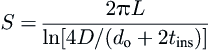$S = \frac{2 π L}{\ln [4 D / (d_{o} + 2 t_{ins})]}$ $S = \frac{2 π L}{\ln [4 D / (d_{o} + 2 t_{ins})]}$

(7.6)

where most of the symbols are as defined previously and D is the depth to which the pipe is buried.

Although soil temperatures vary to some degree with ambient temperature, time of the year (and hence the season), and other factors, these effects are usually neglected. In addition, the soil temperature also varies with location. That is, the soil temperature is different in Texas than it is in Alberta, Canada. In fact, different locations within a state or province may have different soil temperatures. Even the pipeline itself has an effect on the soil temperature.

In the design of a pipeline, it is typical to assume that the soil temperature is a constant. The value used varies from location to location, but for a given pipeline design, it is assumed to be constant.

7.2.1.4. Overall

An approximate value for the overall heat transfer coefficient for an uninsulated pipe is 5 W/m² °C (1 Btu/ft² h °F). For an insulated pipe the heat transfer coefficient is reduced.

For an uninsulated pipeline, the resistance from the soil dominates. Typically, this resistance accounts for more than 90% of the total resistance.

7.2.1.5. Heat Transferred

The energy lost by the fluid to the surroundings can be calculated from the change in enthalpy using the following equation:

$Q = {\dot{m}}_{fluid} (H_{fluid, in} - H_{fluid, out})$ $Q = {\dot{m}}_{fluid} (H_{fluid, in} - H_{fluid, out})$

(7.7)

where

\dot{m}

$\dot{m}$

is the mass flow rate and H is the specific enthalpy.

If there is no phase change, then the enthalpies can be replaced with the product of the temperature and the heat capacity. Equation (7.7) becomes:

$Q = {\dot{m}}_{fluid} C_{fluid} (T_{fluid, in} - T_{fluid, out})$ $Q = {\dot{m}}_{fluid} C_{fluid} (T_{fluid, in} - T_{fluid, out})$

(7.8)

If there is a phase change, then Eqn (7.7) must be used because it accounts for the enthalpy associated with the phase change, whereas Eqn (7.8) does not.

7.2.1.6. Additional Comments

The temperature profile is only one of the many factors that go into the proper design of a pipeline. The optimum design of a pipeline should include all of these considerations.

On the disk accompanying this book is a simple program for calculating the temperature loss from a buried pipeline. This program follows the procedure outlined here. However, it is useful only for performing approximate calculations and should be used with caution. It does not include factors such as the effect of temperature on the properties of the fluid (in the program, they are assumed to be constant). Nor does it account for the possibility of a phase change in the line.

For detailed design, engineers should use software packages that account for all of these effects.

If the pipeline is not buried but exposed to the air or to water, then there is a slight change in the calculation. The term representing the thermal resistance from the soil is replaced with a term for the thermal resistance from the ambient air or water. In still air or water, this convection term is free convection. If the fluid moves, in the case of air by winds and for water by currents, then the convection is forced convection.

7.2.2. Line Heater Design

Figure 7.1 shows a schematic diagram of a line heater. The fire tube is a large diameter U-tube, which is the source of energy for the heater. The fuel gas and air enter the fire tube and are burned to produce the heat.

Figure 7.1 A Schematic Diagram of a Line Heater.

The tube bundle shown in the schematic shows only four tubes but there are usually more than four tubes in the bundle. The tubes in the bundle are typically 50.8–101.6 mm (2–4 in) in diameter. The diameter of the tubes is dictated by the pressure drop and heat transfer considerations. Smaller diameter tubes result in high velocities that in turn result in high pressure drops but also higher heat transfer rates. The wall thickness of the tubes is dependent upon the fluid pressure.

The schematic does not show a choke. With high-pressure gas wells, it is common to produce at high pressure directly into the heater. Then the gas is choked down to pipeline pressure. This pressure reduction will result in cooling of the gas according to the Joule–Thomson effect. The gas then enters a second stage of heating. This is often referred to as “preheat-reheat.” Both the preheat and the reheat take place in the same heater. The amount of heat in the preheat must be such that hydrates do not form after the choke.

The design for the size of the tube bundle begins with the fundamental heat transfer equation (Eqn (7.1)). However, in this case, the log mean temperature difference is calculated as follows:

$Δ T_{lm} = \frac{(T_{fluid, in} - T_{bath}) - (T_{fluid, out} - T_{bath})}{\ln [\frac{T_{fluid, in} - T_{bath}}{T_{fluid, out} - T_{bath}}]} = \frac{T_{fluid, in} - T_{fluid, out}}{\ln [\frac{T_{fluid, in} - T_{bath}}{T_{fluid, out} - T_{bath}}]}$ $Δ T_{lm} = \frac{(T_{fluid, in} - T_{bath}) - (T_{fluid, out} - T_{bath})}{\ln [\frac{T_{fluid, in} - T_{bath}}{T_{fluid, out} - T_{bath}}]} = \frac{T_{fluid, in} - T_{fluid, out}}{\ln [\frac{T_{fluid, in} - T_{bath}}{T_{fluid, out} - T_{bath}}]}$

(7.9)

The subscripts in this equation should be completely descriptive.

A typical bath temperature is about 90 °C (200 °F); however, the bath temperature depends upon the fluid used for the bath. Typically this fluid is water, a glycol, a glycol–water mix, or a specialized heat transfer medium. Clearly, if water is used for the bath, the temperature must be less than 100 °C to prevent all of the water from boiling away.

The overall heat transfer coefficient, U_o, is the sum of four terms: (1) free convection from the bath to the tube bundle, (2) conduction through the pipe, (3) fouling on both sides of the tube, and (4) convection from the fluid flowing in the tube bundle. The U_o is obtained from the following equation:

$\frac{1}{U_{o} A_{o}} = \frac{1}{h_{o} A_{o}} + \frac{\ln (d_{o} / d_{i})}{2 π k_{p} L} + R_{foul} + \frac{1}{h_{i} A_{i}}$ $\frac{1}{U_{o} A_{o}} = \frac{1}{h_{o} A_{o}} + \frac{\ln (d_{o} / d_{i})}{2 π k_{p} L} + R_{foul} + \frac{1}{h_{i} A_{i}}$

(7.10)

The reader should note a similarity between this equation and that for the buried pipeline. The difference between the two equations is the final term, where the term for the resistance from the soil is replaced by the resistance due to the fluid bath.

7.2.2.1. Bath

The tube bundle is in a fluid bath and the heat transfer from the fluid bath to the tubes is via free convection. That is, the flow of the fluid is due to temperature gradients. There is no pump or stirrer to force the flow of the fluid.

The outside heat transfer can be estimated using a correlation for the free convection. There are many correlations for estimating heat transfer coefficients and most all of them can be expressed in the following dimensionless form:

$Nu = f (Gr, \Pr)$ $Nu = f (Gr, \Pr)$

(7.11)

where Nu is the Nusselt number; Gr is the Grashof number, which is a dimensionless number roughly equivalent to the Reynolds number; and Pr is the Prandtl number.

$Nu = C {Gr}^{m} \Pr^{m}$ $Nu = C {Gr}^{m} \Pr^{m}$

(7.12)

values for C and m are given in Table 7.1. Substituting for the dimensionless numbers gives:

$\frac{h_{o} d_{o}}{k} = C {(\frac{g β Δ T d_{o}^{3} ρ^{2}}{μ^{2}})}^{m} {(\frac{C μ}{k})}^{m}$ $\frac{h_{o} d_{o}}{k} = C {(\frac{g β Δ T d_{o}^{3} ρ^{2}}{μ^{2}})}^{m} {(\frac{C μ}{k})}^{m}$

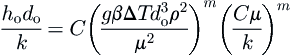(7.13)

Table 7.1

Parameters for Eqn (7.12) for Ranges of Grashof Number Times Prandtl Number

Gr·Pr	C	m
10⁴ to 10⁹	0.53	1/4
10⁹ to 10¹²	0.13	1/3

From Holman (1981).

The properties in this equation are those of the bath fluid and are evaluated at the film temperature (the average between the bath temperature and the temperature of the tube wall). Moreover, d_o is the outside diameter of the tubes, g is the acceleration from gravity (9.81 m/s² or 32.2 ft/s²), β is coefficient of expansion and has units of reciprocal temperature, and all of the other symbols are the same as those given previously. At room temperature, for water, β = 0.2 × 10⁻³/K and for glycol β = 0.65 × 10⁻³/K (Holman, 1981).

7.2.2.2. Tube Bundle

The heat transfer coefficient for the fluid inside the tubes can be calculated using the convection equations discussed previously, which were applicable to the fluid flowing inside of a pipeline.

7.2.2.3. Fire Tube

The area of the fire tube is calculated assuming a flux of 31.5 kW/m² (10,000 Btu/h ft²). Some authors recommend other values (some as low as 25 kW/m²), but 31.5 kW/m² is recommended here.

The minimum fire tube diameter can be estimated as follows (Arnold and Stewart, 1989):

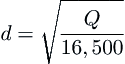$d = \sqrt{\frac{Q}{16, 500}}$ $d = \sqrt{\frac{Q}{16, 500}}$

(7.14)

In this equation, the heat duty, Q, must be in Btu/h and the tube diameter, d, in inches. From the flux, which is the heat transfer rate per unit area, and the diameter, the tube length can be calculated. The fire tube is a U-tube, so the calculated tube length is divided by two and rounded to the nearest foot to obtain the length.

Ultimately, the design of the fire tube is a tradeoff between the tube diameter and length. Smaller diameters result in longer tubes. The design engineer should attempt to fit his or her design to the standard fire tube dimensions. However, if necessary, it is possible to have a custom fire tube constructed.

7.2.2.4. Other Considerations

In the design of any heat exchanger, it is customary to attempt to account for the aging of the exchanger and the buildup of corrosion products, etc., on the exchanger. This is done through the use of a fouling factor, R_foul. Typically the fouling factor for line heaters is approximately 0.0002 m² °C/W (0.001 h ft² °F/Btu).

Finally, the design engineer is wise to confirm all of these values for the various resistances either through the use of heat transfer software, personal experience, or from information provided by vendors.

7.2.2.5. Heat Transfer

The rate of heat transfer to the process fluid can be calculated using Eqn (7.7) or Eqn (7.8).

There is an interesting design twist in the case of preheat-reheat heats. Because the choke valve is an isenthalpic process (constant enthalpy), then the overall energy balance is unaffected. Therefore the heat duty can be estimated based on inlet and outlet conditions only.

7.2.3. Two-Phase Heater Transfer

It is common in both pipeline flow and line heaters that the fluid is not single phase. For a two-phase system, the overall heat transfer coefficient is estimated as a weighted average of those for the two phases (here we assume that the phases are water, W, and gas, G).

$U_{o} = U_{G} (1 - X) + U_{W} X$ $U_{o} = U_{G} (1 - X) + U_{W} X$

(7.15)

where X is the mass fraction of the phase denoted W. The two overall heat transfer coefficients, U_G and U_W, can be calculated using Eqn (7.3) for buried pipelines and Eqn (7.10) for a line heater.

The total heat transfer rate is:

$Q = {\dot{m}}_{G} C_{G} (T_{G, in} - T_{G, out}) + {\dot{m}}_{W} C_{W} (T_{W, in} - T_{W, out})$ $Q = {\dot{m}}_{G} C_{G} (T_{G, in} - T_{G, out}) + {\dot{m}}_{W} C_{W} (T_{W, in} - T_{W, out})$

(7.16)

However, because the two fluids are at the same temperature, this becomes:

$Q = ({\dot{m}}_{G} C_{G} + {\dot{m}}_{W} C_{W}) (T_{fluid, in} - T_{fluid, out})$ $Q = ({\dot{m}}_{G} C_{G} + {\dot{m}}_{W} C_{W}) (T_{fluid, in} - T_{fluid, out})$

(7.17)

Even though these equations seem rather complex, they do not account for exchange between the two phases and thus do not include any latent heat effects. Thus they too should be used with some caution.

7.3. Depressurization

Another method that is used to rid hydrates once they have formed is to reduce the pressure. Based on the information presented earlier, when the pressure is reduced the hydrate is no longer the stable phase. This is different from ice. Depressurizing would have little effect on the freezing point of ice.

Theoretically, this should work, but the process is not instantaneous. It takes some time to melt the hydrate. There are many horror stories about people who depressurized a line and then uncoupled a connection only to have a hydrate projectile shot at them.

Both theory and experiment indicate that the plugs tend to melt radially (from the pipe wall into the center of the pipe) (Peters et al., 2000). The plug shrinks inward but tends to settle to the bottom of the line because of gravity. This forms a flow path for communication between the two sides of the plug, which is typically established quite quickly. In contrast, if the plug melted linearly a flow link would not be established until almost the entire plug had melted.

The porous-permeable nature of most hydrate plugs means that there can be some flow communication through the plug and this tends to equalize pressures on both sides. However, it is unwise to assume that this will be the case, because it the rare case the plug is not very permeable.

Typically, the lower the pressure the faster the plug melts. However, when the pressure is reduced, there is a cooling resulting from the Joule–Thomson effect (see Chapter 11). If the depressurizing is done quickly, there is no time to equilibrate with the surroundings and one must wait for the system to warm.

A potentially dangerous scenario for the melting of a hydrate plug using pressure reduction is presented in Fig. 7.2. As shown in the figure, an attempt is made to melt the hydrate blockage by bleeding the pressure off the line.

However, in this case, the pressure is only bled off one side of the hydrate. The plug can loosen and will be projected along the line at high velocity. The hydrate can accelerate along the line like a bullet in a rifle barrel. The speed of the plug can often be enhanced by a fine film of water that acts as a lubricant.

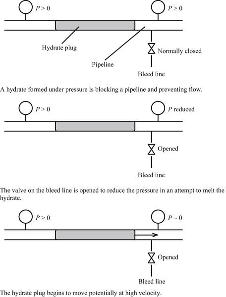
Figure 7.2 Improper Depressurization of Hydrate Plug Resulting in the Hydrate Plug Being Launched Like a Projectile.

In this situation, it is better if the pressure is bled off both sides of the blockage. And if possible an attempt should be made to keep the pressure nearly equal on both sides of the plug. Maintaining equal pressure on both sides will prevent significant movement of the plug. Based on experience, a maximum of 10% difference in the pressure across a hydrate plug is commonly specified, but it would not be classified as an “industry standard.”

If it is not possible to bleed off both sides of the line, then the pressure should bled off one side of the plug in a step-like manner. First, release some pressure and allow the plug to melt, which will increase the pressure. Then more pressure is released. Continue to step down in pressure until the plug melts. The problem with this method is that sufficient pressure must be bled off that hydrate melting will occur but not result in the plug becoming a projectile. If the pressure in the line is well above the hydrate formation pressure, then bleeding off some pressure will not melt the hydrate. If the line pressure is high, even bleeding of 1400–2000 kPa (200–300 psia), which is sufficient to create a dangerous projectile, may not be enough to melt the blockage. Therefore, it is important to know the hydrate formation pressure in order to know how much pressure to bleed.

Standard procedures are in place in most jurisdictions that are designed to prevent accidents during the maintenance of oil field equipment. Often, operating companies have even more stringent procedures for contractors working in their employ. It is wise to follow such procedures.

7.4. Melting a Plug with Heat

Another method to remove a hydrate plug is to melt it with the application of heat. Heat can be applied by spraying steam on the line or electrical resistance heating or the like. However, this method should also be used with caution. A potentially dangerous situation is depicted in Fig. 7.3.

The melted plug will release gas and produce liquid water. As will be demonstrated in Chapter 8, 1 m³ [act] of methane hydrate releases 170 Sm³ of gas. The melting also produces 51.45 kmol of liquid water, which occupies 0.927 m³ as a liquid. This means that if the hydrate is melted in a confined space, there is only 0.073 m³ available for the 170 Sm³ of released gas.

The pressure of the released gas can be crudely estimated using the ideal gas law:

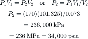
$\begin{matrix} P_{1} V_{1} = P_{2} V_{2} or P_{2} = P_{1} V_{1} / V_{2} \\ P_{2} = (170) (101.325) / 0.073 \\ = 236, 000 kPa \\ = 236 MPa = 34, 000 psia \end{matrix}$ $\begin{matrix} P_{1} V_{1} = P_{2} V_{2} or P_{2} = P_{1} V_{1} / V_{2} \\ P_{2} = (170) (101.325) / 0.073 \\ = 236, 000 kPa \\ = 236 MPa = 34, 000 psia \end{matrix}$

Although there are some errors in this analysis, it provides better than an order of magnitude estimate of the pressure buildup. And as can be seen, the pressure is very large and capable of bursting most pipes.

If you redo the calculation, you will see that the calculated pressure is independent of the volume melted as long as the melting occurs in a confined space. Therefore do not think the problem is reduced if a volume less than 1 m³ is melted—this is not the case. Even melting a very small volume will result in the same dangerous over pressurization.

Figure 7.3 Scenario for Pipeline Rupture during the Melting of a Gas Hydrate Plug.

Those more familiar with American Engineering Units can redo the calculation and see that the result is also independent of the set of units used. Melting a hydrate in a confined space results in a large over pressurization regardless of the set of units used for the calculation.

On the other hand, if the hydrate plug can move, then this becomes similar to the scenario shown in Fig. 7.2. The pressure buildup in the melted section can result in a hydrate projectile. Again the hydrate is projected like a bullet with a significant potential for causing damage.

To avoid these dangerous situations, it is important to heat the entire hydrate plug. When heating externally, this may be difficult because it requires locating the entire plug within the pipeline. It is wise to heat more of the line rather than less. Err on the side of caution. Heat more line than you believe is occupied by the gas hydrate plug.

7.5. Hydrate Plug Location

As was demonstrated in the examples previously, it is important to do your best to locate the hydrate plug. It is difficult if not impossible to determine the exact location of a hydrate plug. However, with some engineering tools and Sherlock Holmes-like deduction, a best estimate of the plug location can be determined. Some guidelines are presented in this section.

If you have access to the pipe, a temperature survey may reveal the location of the hydrate. However, if the pipeline is buried, this maybe a difficult problem. Thus some preliminary analysis of the situation may lead to possible locations for the hydrate plug. Flow modeling should indicate where the flow conditions cross the hydrate curve. However, the point when hydrates begin to form is not where they will accumulate. Likely locations for the hydrates to accumulate are low points in the pipe or constriction from fitting or valves. These locations should be checked first.

If the line is exposed, the temperature can be measured using an infrared temperature “gun.” One simply points the gun at the pipeline and obtains a surface temperature for the pipe. A cold spot in the line would be indicative of a hydrate plug.

7.6. Buildings

In colder climates, such as Western Canada, it is common to house process equipment, field batteries, and even wells along with some of their associated facilities in heated buildings. The buildings not only provide comfort to operators during inclement weather, they also can prevent freezing of the equipment.

In the early gas industry in Western Canada, the plants were constructed in the style of warmer climates. That is, they were built without building. Freezing was a serious problem. This freezing was not all from hydrate formation, but some of it almost certainly was. Since that time, most gas plants in Western Canada are constructed with buildings and the interior of the buildings is heated.

7.7. Capital Costs

Figure 7.4 gives quick estimates (±30%) for the purchased cost of a line heater. This chart is based partially on information from the literature, but largely from the experience of the author.

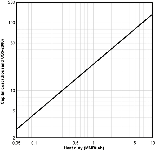
Figure 7.4 Approximate Capital Cost for Line Heaters.

As an order of magnitude estimate, it can be assumed that the installation cost is between 0.8 and 1.2 times the purchased cost. In other words, the installation cost is approximately equal to the purchased cost.

Clearly, these costs are approximations at best. Many factors have not been included such as the operating pressure, gas flow rate, etc. They should be used for rapid budget cost estimates only.

7.8. Case Studies

7.8.1. Case 1

The National Energy Board of Canada (2004) reported an incident that occurred in British Columbia. An 18-in pipeline (DN 450) ruptured, and the force from the blast was sufficient to knock down a nearby worker who was unhurt. The pipeline was transporting sour gas (0.4% H₂S), which was released to the environment. An emergency situation was triggered and nearby residences were evacuated. Fortunately no one was adversely affected by the release.

The investigation revealed that the likely cause was due to a shock wave after a hydrate plug was released by high differential pressure. It also concluded that the point where the pipeline burst was probably a weak point from a manufacturer defect.

The Board recommends that companies develop procedures for melting hydrate plugs and that the procedures are followed.

The hydrate plug must have been of significant size to block an 18-in line.

7.8.2. Case 2

The Edmonton Journal (Sands, 2011) reported an incident near Fox Creek, Alberta. According to an article, a crew was sent to a pipeline to melt an “ice plug” inside the pipe. They used steam wands to melt the “ice” (i.e., steam was directly applied to the pipe at the suspected location of the plug), which resulted in a release of sour gas. The leak was deadly—one of the workers died as a result of H₂S poisoning. Others, including a policeman investigating the situation, were sent to hospital.

The newspaper article is intended for a general audience and requires some interpretation. First, because this was a natural gas pipeline, it is safe to assume that it was not ice but hydrate that blocked the line. Other details in the article are a little thin, but this appears to be a case of improperly locating the hydrate and melting from a more or less central point. The overpressure resulted in a pipeline leak.

Furthermore, although the article does not mention defects in the pipe, it is possible that a manufacturer's defect contributed to the failure, as was the case in the previous incident.

However, this incident demonstrates the need for locating the hydrate plug before melting it. Also care should be taken not to melt the plug too fast, which would result in an over pressurization of the line.

Examples

Example 7.1

Gas is to flow at a rate of 195.7 × 10³ Sm³/day (6.91 MMCFD) in a buried pipeline from a well site to a gas plant 7.5 km (4.66 miles) away. From other considerations (pressure drop, wall thickness, etc.), it is decided to use 4-in schedule 80 pipe (k = 48.5 W/m K). The gas at the wellhead is at 48.89 °C (120 °F) and 7500 kPa (1087 psia).

From the methods presented earlier, it is determined that at the pressure in the pipeline a hydrate will form at 15 °C (59 °F).

Table 7.2

Properties of the Natural Gas for Example 7.1

	SI Unit	Engineering Units
Density	68.1 kg/m³	4.25 lb/ft³
Molar Mass	23.62 kg/kmol	23.62 lb/lb mol
Heat Capacity	2.76 kJ/kg K	0.66 Btu/lb °F
Viscosity	0.013 mPa s	0.013 cP
Thermal Conductivity	0.040 W/m K	0.023 Btu/h ft °F

If the pipeline is uninsulated, estimate the temperature of the gas arriving at the plant. Furthermore, estimate the thickness of insulation (k = 0.173 W/m K) required such that the gas will arrive at the plant 5 °C (9 °F) above the hydrate temperature. That is, such that the gas arrives at the plant at 20 °C.

The physical properties of the gas are given in Table 7.2. The soil temperature is 1.67 °C (35 °F) and the thermal conductivity of the soil is 1.3 W/m K.

Answer: First, convert the flow rate from volumetric to a mass flow.

$\dot{n} = \frac{P v}{R T} = \frac{(101.325) (195.7 \times 10^{3})}{(8.314) (15.55 + 273.15)} = 8261.3 kmol/day$ $\dot{n} = \frac{P v}{R T} = \frac{(101.325) (195.7 \times 10^{3})}{(8.314) (15.55 + 273.15)} = 8261.3 kmol/day$

$\dot{m} = \frac{(8260.3) (24)}{20.363} = 9737 kg/h$ $\dot{m} = \frac{(8260.3) (24)}{20.363} = 9737 kg/h$

From standard tables for pipe properties, a 4-in schedule 80 pipe has an outside diameter of 11.430 cm (4.50 in) and an inside diameter of 9.718 cm (3.826 in).

All of the other information required for the program is given in the statement of the problem or in Table 7.2. In general, the design engineer would be required to find these values in reference books or calculate the properties.

The program on the enclosed disk can be used to perform this calculation. The output from this run is appended to this chapter. From the output the exit temperature is estimated to be 8.1 °C, well below the hydrate formation temperature.

Three cases of insulated pipe were also examined: 2.54 cm (1 in) of insulation, 5.08 cm (2 in), and 7.62 cm (3 in). The enclosed program was used for these cases as well. The complete output is also in the appendix and the outlet temperatures are summarized below:

No Insulation	8.1 °C
2.54 cm	15.0 °C
5.08 cm	19.0 °C
7.62 cm	21.7 °C

Therefore 5.08 cm (2 in) of insulation is not quite enough and 7.62 cm (3 in) is too much.

Figure 7.5 Temperature Loss along the Pipeline for Example 7.1.

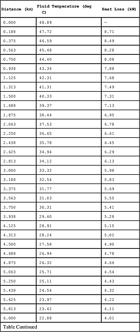
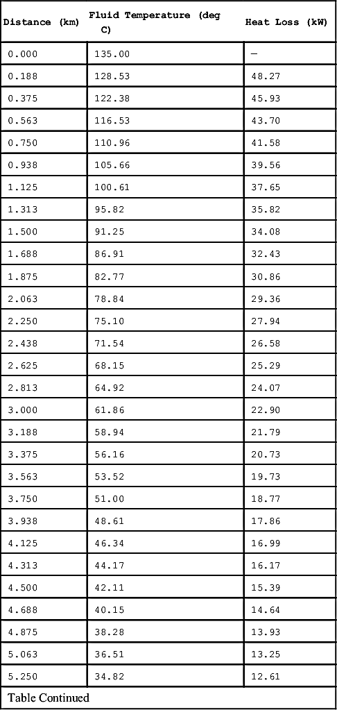
Finally, Fig. 7.5 is a plot showing the temperature along the pipeline for the four cases. In addition, the reader is invited to review the complete output listed in the Appendix to obtain further insights into the heat loss from pipelines in general and the results for this specific case.

Example 7.2

As an alternative to insulating the line, it is suggested that a heater be used. How hot should the inlet gas be heated to in order to arrive at the plant 5 °C above the expected hydrate formation temperature?

Answer: Again the program on the accompanying disk is used for this calculation. However, this requires an iterative solution.

Inlet Temperature	Outlet Temperature
48.89	8.13—This is from Example 7.1.
100	15.15
200	28.82
135	9.92—This value of 135 °C obtained by linearly interpolating the previous two values.

At this point, it is worth commenting that there are limits to the temperature that the gas can enter a pipeline. One concern is that high temperatures damage the yellow jacket. Furthermore, to obtain a fluid temperature of 135 °C would require a bath temperature of at least 140 °C (an approach temperature of 5 °C). Clearly, to obtain this temperature, the bath fluid cannot be water.

Example 7.3

Estimate the duty required to heat the gas from 48.89 to 135 °C. Furthermore, estimate the capital cost of the line heater required.

Answer: First calculate the heat duty using Eqn (7.8):

$\begin{matrix} Q = (9737 kg/h) (2.76 kJ/kg K) (135 - 48.89) = 2, 314, 000 kJ/h \\ = 643, 000 W = 643 kW \end{matrix}$ $\begin{matrix} Q = (9737 kg/h) (2.76 kJ/kg K) (135 - 48.89) = 2, 314, 000 kJ/h \\ = 643, 000 W = 643 kW \end{matrix}$

Convert to engineering units:

$Q = 2.192 MMBtu/h$ $Q = 2.192 MMBtu/h$

From Fig. 7.2 the approximate capital cost is $35,000 (US) (about $52,500 Cdn).

Appendix 7A Output from Pipe Heat Loss Program for the Examples in the Text

   ∗∗∗∗∗∗∗∗∗∗∗∗∗∗∗∗∗∗∗∗∗∗∗∗∗∗∗∗∗∗∗∗∗∗∗∗∗∗∗∗∗∗∗∗∗∗∗∗∗
   ∗∗   Buried Pipeline Heat Loss Calculation  ∗∗
   ∗∗   Vers. 1.1          Sept. 2000   ∗∗
   ∗∗   ----------- BETA RELEASE------------   ∗∗
   ∗∗∗∗∗∗∗∗∗∗∗∗∗∗∗∗∗∗∗∗∗∗∗∗∗∗∗∗∗∗∗∗∗∗∗∗∗∗∗∗∗∗∗∗∗∗∗∗∗
 Project: Field Book Example
 Job Number: 01234   Date: 07-11-2001   Time: 09:01:03
 INPUT PARAMETERS:
 ------------------
 Fluid Properties:
 ------------------

Heat Capacity (kJ/kg-K)	2.76
Viscosity (cp)	0.013
Density (kg/m³)	68.1
Thermal Conductivity (W/m-K)	0.04
Mass Flow Rate (kg/hr)	9737
Fluid Temperature (deg C)	48.89

 Pipe Properties:
 -----------------

Inside Diameter (cm)	9.718
Outside Diameter (cm)	11.43
Thermal Conductivity (W/m-K)	48.5
Buried Depth (m)	1.5
Length (km)	7.5

 Insulation Properties:
 ----------------------
 ∗∗∗ Pipe Uninsulated ∗∗∗
 Yellow Jacket:
 --------------
 Pipe coated with Yellow Jacket
 Soil Properties:
 ----------------

Thermal Conductivity (W/m-K)	1.3
Temperature (deg C)	1.67

 CALCULATED RESULTS:
 -------------------

Fluid Exit Temperature	8.13 deg C
Temperature Change	40.76 deg C
Log Mean Temperature Change	20.50 deg C

Reynolds Number	2.726E+06
Prandtl Number	8.970E−01
Nusselt Number	3.133E+03

Fluid Velocity	5.355 m/s
Pressure Drop	1.726E+02 Pa/m	∗∗∗Approximate∗∗∗
Total Pressure Drop	1.295E+03 kPa	∗∗∗Approximate∗∗∗

Inside Heat Transfer Coeff	1.290E+03 W/m²-K
Inside Overall Heat Transfer Coeff	6.483E+00 W/m²-K
Inside Surface Area	2.290E+03 m²
Outside Overall Heat Transfer Coeff	5.392E+00 W/m²-K
Outside Surface Area	2.753E+03 m²
Total Heat Transfer	3.042E+02 kW

 Pipeline Profile
 ----------------

Distance (km)	Fluid Temperature (deg C)	Heat Loss (kW)
0.000	48.89	–
0.188	46.60	17.09
0.375	44.42	16.27
0.563	42.35	15.48
0.750	40.38	14.73
0.938	38.50	14.01
1.125	36.71	13.33
1.313	35.01	12.69
1.500	33.40	12.07
1.688	31.86	11.49
1.875	30.39	10.93
2.063	29.00	10.40
2.250	27.67	9.89
2.438	26.41	9.41
2.625	25.21	8.96
2.813	24.07	8.52
3.000	22.99	8.11
3.188	21.95	7.72
3.375	20.97	7.34
3.563	20.03	6.99
3.750	19.14	6.65
3.938	18.29	6.33
4.125	17.49	6.02
4.313	16.72	5.73
4.500	15.99	5.45
4.688	15.30	5.18
4.875	14.64	4.93
5.063	14.01	4.69
5.250	13.41	4.47
5.438	12.84	4.25
5.625	12.30	4.04
5.813	11.78	3.85
6.000	11.29	3.66
6.188	10.83	3.48
6.375	10.38	3.31
6.563	9.96	3.15
6.750	9.56	3.00
6.938	9.17	2.86
7.125	8.81	2.72
7.313	8.46	2.59
7.500	8.13	2.46

Contributions to Overall Heat Transfer Coefficient:
----------------------------------------------------

Resistance Due to Fluid	0.50%
Resistance Due to Pipe	0.11%
Resistance Due to Insulation	0.00%
Resistance Due to Yellow Jacket	3.96%
Resistance Due to Soil	95.44%

   ∗∗∗∗∗∗∗∗∗∗∗∗∗∗∗∗∗∗∗∗∗∗∗∗∗∗∗∗∗∗∗∗∗∗∗∗∗∗∗∗∗∗∗∗∗∗∗∗∗
   ∗∗   Buried Pipeline Heat Loss Calculation  ∗∗
   ∗∗   Vers. 1.1         Sept. 2000    ∗∗
   ∗∗   ----------- BETA RELEASE ------------  ∗∗
   ∗∗∗∗∗∗∗∗∗∗∗∗∗∗∗∗∗∗∗∗∗∗∗∗∗∗∗∗∗∗∗∗∗∗∗∗∗∗∗∗∗∗∗∗∗∗∗∗∗
 Project: Field Book Example

Job Number: 01234 Date: 07-11-2001 Time: 09:10:07

 INPUT PARAMETERS:
 -----------------
 Fluid Properties:
 -----------------

Heat Capacity (kJ/kg-K)	2.76
Viscosity (cp)	0.013
Density (kg/m³)	68.1
Thermal Conductivity (W/m-K)	0.04
Mass Flow Rate (kg/hr)	9737
Fluid Temperature (deg C)	48.89

 Pipe Properties:
 ----------------

Inside Diameter (cm)	9.718
Outside Diameter (cm)	11.43
Thermal Conductivity (W/m-K)	48.5
Buried Depth (m)	1.5
Length (km)	7.5

 Insulation Properties:
 ----------------------

Thermal Conductivity (W/m-K)	0.173
Insulation Thickness (cm)	2.54

 Yellow Jacket:
 --------------
 Pipe coated with Yellow Jacket
 Soil Properties:
 ----------------

Thermal Conductivity (W/m-K)	1.3
Temperature (deg C)	1.67

 CALCULATED RESULTS:
 -------------------

Fluid Exit Temperature	14.98 deg C
Temperature Change	33.91 deg C
Log Mean Temperature Change	26.78 deg C

Reynolds Number	2.726E+06
Prandtl Number	8.970E−01
Nusselt Number	3.133E+03

Fluid Velocity	5.355 m/s
Pressure Drop	1.726E+02 Pa/m	∗∗∗Approximate∗∗∗
Total Pressure Drop	1.295E+03 kPa	∗∗∗Approximate∗∗∗

Inside Heat Transfer Coeff	1.290E+03 W/m²-K
Inside Overall Heat Transfer Coeff	4.129E+00 W/m²-K
Inside Surface Area	2.290E+03 m²
Outside Overall Heat Transfer Coeff	2.394E+00 W/m²-K
Outside Surface Area	3.950E+03 m²
Total Heat Transfer	2.532E+02 kW

 Pipeline Profile
 ----------------

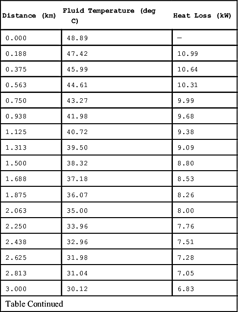
Distance (km)	Fluid Temperature (deg C)	Heat Loss (kW)
0.000	48.89	–
0.188	47.42	10.99
0.375	45.99	10.64
0.563	44.61	10.31
0.750	43.27	9.99
0.938	41.98	9.68
1.125	40.72	9.38
1.313	39.50	9.09
1.500	38.32	8.80
1.688	37.18	8.53
1.875	36.07	8.26
2.063	35.00	8.00
2.250	33.96	7.76
2.438	32.96	7.51
2.625	31.98	7.28
2.813	31.04	7.05
3.000	30.12	6.83
Table Continued

Distance (km)	Fluid Temperature (deg C)	Heat Loss (kW)
3.188	29.23	6.62
3.375	28.38	6.41
3.563	27.54	6.21
3.750	26.74	6.02
3.938	25.96	5.83
4.125	25.20	5.65
4.313	24.47	5.47
4.500	23.76	5.30
4.688	23.07	5.14
4.875	22.40	4.98
5.063	21.75	4.82
5.250	21.13	4.67
5.438	20.52	4.53
5.625	19.93	4.39
5.813	19.36	4.25
6.000	18.81	4.12
6.188	18.28	3.99
6.375	17.76	3.86
6.563	17.26	3.74
6.750	16.77	3.63
6.938	16.30	3.51
7.125	15.85	3.40
7.313	15.41	3.30
7.500	14.98	3.20

 Contributions to Overall Heat Transfer Coefficient:
 ----------------------------------------------------

Resistance Due to Fluid	0.32%
Resistance Due to Pipe	0.07%
Resistance Due to Insulation	42.65%
Resistance Due to Yellow Jacket	1.75%
Resistance Due to Soil	55.22%

   ∗∗∗∗∗∗∗∗∗∗∗∗∗∗∗∗∗∗∗∗∗∗∗∗∗∗∗∗∗∗∗∗∗∗∗∗∗∗∗∗∗∗∗∗∗∗∗∗∗
   ∗∗   Buried Pipeline Heat Loss Calculation  ∗∗
   ∗∗   Vers. 1.1         Sept. 2000    ∗∗
   ∗∗   ----------- BETA RELEASE ------------  ∗∗
   ∗∗∗∗∗∗∗∗∗∗∗∗∗∗∗∗∗∗∗∗∗∗∗∗∗∗∗∗∗∗∗∗∗∗∗∗∗∗∗∗∗∗∗∗∗∗∗∗∗
 Project: Field Book Example
 Job Number: 01234   Date: 07-11-2001   Time: 09:13:24
 INPUT PARAMETERS:
 -----------------

 Fluid Properties:
 -----------------

Heat Capacity (kJ/kg-K)	2.76
Viscosity (cp)	0.013
Density (kg/m³)	68.1
Thermal Conductivity (W/m-K)	0.04
Mass Flow Rate (kg/hr)	9737
Fluid Temperature (deg C)	48.89

 Pipe Properties:
 ----------------

Inside Diameter (cm)	9.718
Outside Diameter (cm)	11.43
Thermal Conductivity (W/m-K)	48.5
Buried Depth (m)	1.5
Length (km)	7.5

 Insulation Properties:
 ----------------------

Thermal Conductivity (W/m-K)	0.173
Insulation Thickness (cm)	5.08

 Yellow Jacket:
 --------------
 Pipe coated with Yellow Jacket
 Soil Properties:
 ----------------

Thermal Conductivity (W/m-K)	1.3
Temperature (deg C)	1.67

CALCULATED RESULTS:
-------------------

Fluid Exit Temperature	19.04 deg C
Temperature Change	29.85 deg C
Log Mean Temperature Change	29.85 deg C

Reynolds Number	2.726E+06
Prandtl Number	8.970E−01
Nusselt Number	3.133E+03

Fluid Velocity	5.355 m/s
Pressure Drop	1.726E+02 Pa/m	∗∗∗Approximate∗∗∗
Total Pressure Drop	1.295E+03 kPa	∗∗∗Approximate∗∗∗

Inside Heat Transfer Coeff	1.290E+03 W/m²-K
Inside Overall Heat Transfer Coeff	3.261E+00 W/m²-K
Inside Surface Area	2.290E+03 m²
Outside Overall Heat Transfer Coeff	1.451E+00 W/m²-K
Outside Surface Area	5.147E+03 m²
Total Heat Transfer	2.229E+02 kW

Pipeline Profile.

  ----------------

Distance (km)	Fluid Temperature (deg C)	Heat Loss (kW)
0.000	48.89	–
0.188	47.72	8.71
0.375	46.59	8.49
0.563	45.48	8.28
0.750	44.40	8.08
0.938	43.34	7.88
1.125	42.31	7.68
1.313	41.31	7.49
1.500	40.33	7.31
1.688	39.37	7.13
1.875	38.44	6.95
2.063	37.53	6.78
2.250	36.65	6.61
2.438	35.78	6.45
2.625	34.94	6.29
2.813	34.12	6.13
3.000	33.32	5.98
3.188	32.54	5.83
3.375	31.77	5.69
3.563	31.03	5.55
3.750	30.31	5.41
3.938	29.60	5.28
4.125	28.91	5.15
4.313	28.24	5.02
4.500	27.58	4.90
4.688	26.94	4.78
4.875	26.32	4.66
5.063	25.71	4.54
5.250	25.11	4.43
5.438	24.54	4.32
5.625	23.97	4.22
5.813	23.42	4.11
6.000	22.88	4.01
Table Continued

Distance (km)	Fluid Temperature (deg C)	Heat Loss (kW)
6.188	22.36	3.91
6.375	21.85	3.81
6.563	21.35	3.72
6.750	20.86	3.63
6.938	20.39	3.54
7.125	19.93	3.45
7.313	19.48	3.37
7.500	19.04	3.28

 Contributions to Overall Heat Transfer Coefficient:
 ----------------------------------------------------

Resistance Due to Fluid	0.25%
Resistance Due to Pipe	0.05%
Resistance Due to Insulation	58.25%
Resistance Due to Yellow Jacket	1.06%
Resistance Due to Soil	40.38%

   ∗∗∗∗∗∗∗∗∗∗∗∗∗∗∗∗∗∗∗∗∗∗∗∗∗∗∗∗∗∗∗∗∗∗∗∗∗∗∗∗∗∗∗∗∗∗∗∗∗
   ∗∗  Buried Pipeline Heat Loss Calculation   ∗∗
   ∗∗  Vers. 1.1          Sept. 2000   ∗∗
   ∗∗  ----------- BETA RELEASE ------------   ∗∗
   ∗∗∗∗∗∗∗∗∗∗∗∗∗∗∗∗∗∗∗∗∗∗∗∗∗∗∗∗∗∗∗∗∗∗∗∗∗∗∗∗∗∗∗∗∗∗∗∗∗
 Project: Field Book Example
 Job Number: 01234   Date: 07-11-2001   Time: 09:26:12
 INPUT PARAMETERS:
 -----------------
 Fluid Properties:
 -----------------

Heat Capacity (kJ/kg-K)	2.76
Viscosity (cp)	0.013
Density (kg/m³)	68.1
Thermal Conductivity (W/m-K)	0.04
Mass Flow Rate (kg/hr)	9737
Fluid Temperature (deg C)	48.89

 Pipe Properties:
 ----------------

Inside Diameter (cm)	9.718
Outside Diameter (cm)	11.43
Thermal Conductivity (W/m-K)	48.5
Buried Depth (m)	1.5
Length (km)	7.5

 Insulation Properties:
 ----------------------

Thermal Conductivity (W/m-K)	0.173
Insulation Thickness (cm)	7.62

 Yellow Jacket:
 --------------
 Pipe coated with Yellow Jacket
 Soil Properties:
 ----------------

Thermal Conductivity (W/m-K)	1.3
Temperature (deg C)	1.67

 CALCULATED RESULTS:
 -------------------

Fluid Exit Temperature	21.69 deg C
Temperature Change	27.20 deg C
Log Mean Temperature Change	31.70 deg C

Reynolds Number	2.726E+06
Prandtl Number	8.970E−01
Nusselt Number	3.133E+03

Fluid Velocity	5.355 m/s
Pressure Drop	1.726E+02 Pa/m	∗∗∗Approximate∗∗∗
Total Pressure Drop	1.295E+03 kPa	∗∗∗Spproximate∗∗∗

Inside Heat Transfer Coeff	1.290E+03 W/m²-K
Inside Overall Heat TransferCoeff	2.797E+00 W/m²-K
Inside Surface Area	2.290E+03 m²
Outside Overall Heat TransferCoeff	1.009E+00 W/m²-K
Outside Surface Area	6.344E+03 m²
Total Heat Transfer	2.030E+02 kW

 Pipeline Profile
 ----------------

Distance (km)	Fluid Temperature (deg C)	Heat Loss (kW)
0.000	48.89	–
0.188	47.89	7.48
0.375	46.91	7.32
0.563	45.95	7.17
0.750	45.01	7.01
0.938	44.09	6.86
1.125	43.19	6.72
1.313	42.31	6.58
Table Continued

Distance (km)	Fluid Temperature (deg C)	Heat Loss (kW)
1.500	41.45	6.44
1.688	40.60	6.30
1.875	39.78	6.17
2.063	38.97	6.04
2.250	38.18	5.91
2.438	37.40	5.78
2.625	36.64	5.66
2.813	35.90	5.54
3.000	35.17	5.42
3.188	34.46	5.31
3.375	33.77	5.19
3.563	33.09	5.08
3.750	32.42	4.98
3.938	31.77	4.87
4.125	31.13	4.77
4.313	30.50	4.67
4.500	29.89	4.57
4.688	29.29	4.47
4.875	28.71	4.38
5.063	28.13	4.28
5.250	27.57	4.19
5.438	27.02	4.10
5.625	26.48	4.02
5.813	25.96	3.93
6.000	25.44	3.85
6.188	24.94	3.77
6.375	24.44	3.69
6.563	23.96	3.61
6.750	23.49	3.53
6.938	23.03	3.46
7.125	22.57	3.38
7.313	22.13	3.31
7.500	21.69	3.24

 Contributions to Overall Heat Transfer Coefficient:
 ----------------------------------------------------

Resistance Due to Fluid	0.22%
Resistance Due to Pipe	0.05%
Resistance Due to Insulation	66.56%
Resistance Due to Yellow Jacket	0.74%
Resistance Due to Soil	32.45%

   ∗∗∗∗∗∗∗∗∗∗∗∗∗∗∗∗∗∗∗∗∗∗∗∗∗∗∗∗∗∗∗∗∗∗∗∗∗∗∗∗∗∗∗∗∗∗∗∗∗
   ∗∗  Buried Pipeline Heat Loss Calculation   ∗∗
   ∗∗  Vers. 1.1          Sept. 2000    ∗∗
   ∗∗  ----------- BETA RELEASE ------------   ∗∗
   ∗∗∗∗∗∗∗∗∗∗∗∗∗∗∗∗∗∗∗∗∗∗∗∗∗∗∗∗∗∗∗∗∗∗∗∗∗∗∗∗∗∗∗∗∗∗∗∗∗
 Project: Field Book Example
 Job Number: 01234   Date: 07-11-2001   Time: 10:42:23
 INPUT PARAMETERS:
 -----------------
 Fluid Properties:
 -----------------

Heat Capacity (kJ/kg-K)	2.76
Viscosity (cp)	0.013
Density (kg/m³)	68.1
Thermal Conductivity (W/m-K)	0.04
Mass Flow Rate (kg/hr)	9737
Fluid Temperature (deg C)	135

 Pipe Properties:
 ----------------

Inside Diameter (cm)	9.718
Outside Diameter (cm)	11.43
Thermal Conductivity (W/m-K)	48.5
Buried Depth (m)	1.5
Length (km)	7.5

 Insulation Properties:
 ----------------------
 ∗∗∗ Pipe Uninsulated ∗∗∗
 Yellow Jacket:
 --------------
 Pipe coated with Yellow Jacket
 Soil Properties:
 ----------------

Thermal Conductivity (W/m-K)	1.3
Temperature (deg C)	1.67

 CALCULATED RESULTS:
 -------------------

Fluid Exit Temperature	19.92deg C
Temperature Change	115.08 deg C
Log Mean Temperature Change	57.87deg C

Reynolds Number	2.726E+06
Prandtl Number	8.970E−01
Nusselt Number	3.133E+03

Fluid Velocity	5.355 m/s
Pressure Drop	1.726E+02 Pa/m	∗∗∗Approximate∗∗∗
Total Pressure Drop	1.295E+03 kPa	∗∗∗Approximate∗∗∗

Inside Heat Transfer Coeff	1.290E+03 W/m²-K
Inside Overall Heat Transfer Coeff	6.483E+00 W/m²-K
Inside Surface Area	2.290E+03 m²
Outside Overall Heat Transfer Coeff	5.392E+00 W/m²-K
Outside Surface Area	2.753E+03 m²
Total Heat Transfer	8.590E+02 kW

 Pipeline Profile
 ----------------

Distance (km)	Fluid Temperature (deg C)	Heat Loss (kW)
0.000	135.00	–
0.188	128.53	48.27
0.375	122.38	45.93
0.563	116.53	43.70
0.750	110.96	41.58
0.938	105.66	39.56
1.125	100.61	37.65
1.313	95.82	35.82
1.500	91.25	34.08
1.688	86.91	32.43
1.875	82.77	30.86
2.063	78.84	29.36
2.250	75.10	27.94
2.438	71.54	26.58
2.625	68.15	25.29
2.813	64.92	24.07
3.000	61.86	22.90
3.188	58.94	21.79
3.375	56.16	20.73
3.563	53.52	19.73
3.750	51.00	18.77
3.938	48.61	17.86
4.125	46.34	16.99
4.313	44.17	16.17
4.500	42.11	15.39
4.688	40.15	14.64
4.875	38.28	13.93
5.063	36.51	13.25
5.250	34.82	12.61
Table Continued

Distance (km)	Fluid Temperature (deg C)	Heat Loss (kW)
5.438	33.21	12.00
5.625	31.68	11.42
5.813	30.22	10.86
6.000	28.84	10.34
6.188	27.52	9.84
6.375	26.27	9.36
6.563	25.08	8.90
6.750	23.94	8.47
6.938	22.86	8.06
7.125	21.83	7.67
7.313	20.85	7.30
7.500	19.92	6.95

 Contributions to Overall Heat Transfer Coefficient:
 ----------------------------------------------------

Resistance Due to Fluid	0.50%
Resistance Due to Pipe	0.11%
Resistance Due to Insulation	0.00%
Resistance Due to Yellow Jacket	3.96%
Resistance Due to Soil	95.44%

..................Content has been hidden....................

You can't read the all page of ebook, please click here login for view all page.

Table of Contents for Chapter 7. Combating Hydrates Using Heat and Pressure

Create new playlist

Sign In

Sign Up