
Chapter 11
Additional Topics
Abstract
This chapter is a collection of other topics related to gas hydrates. Subjects include the Joule–Thomson effect, hydrates in nature (both terrestrial and extraterrestrial), the formation of hydrates during gas production (both in the formation and in the well), and the potential for storing carbon dioxide as a hydrate in a subsurface reservoir for the purposes of sequestering it.
Keywords
Carbon sequestration; Gas well; Joule–thomson effect; Seabed hydratesIn this final chapter, we will review some additional topics that do not fit into the earlier chapters, but are of importance to the topic of gas hydrates.
11.1. Joule-Thomson Expansion
When a fluid flows through a valve (or, as in the original experiments, a porous plug or any restriction to the flow), the fluid pressure drops. The process occurs adiabatically, that is without heat being transferred. This is because it happens quite quickly. The process is shown graphically in Fig. 11.1. The question is now what happens to the temperature of the fluid during such a process?
If you are unaware of the Joule–Thomson effect, but have some technical knowledge, you might conclude that the temperature is unchanged by the throttling process. There appears to be nothing happening to change the temperature of the fluid. This view is incorrect, except in a few relatively rare cases.
On the other hand, it should be clear to all that no work is done as the fluid crosses the valve. The potential work available from going from high pressure to low pressure is simply lost.
Those with some technical training might say that the fluid cools upon such an expansion and that the temperature leaving the valve is lower than that entering.

11.2. Theoretical Treatment
The detailed thermodynamics of the Joule–Thomson expansion are well understood. Those interested can check almost any book on classical thermodynamics, but the details are outlined here briefly.
Mathematically this is given by:
 (11.1)
When this quantity is positive, the fluid cools upon expansion, and when it is negative, the fluid warms.
From classical thermodynamics, we can derive the following expression for this quantity:
 (11.2)
The derivation of this expression is given in most textbooks on classical thermodynamics and will not be repeated here.
We have reduced the expression to one that contains only the pressure, temperature, molar volume (and derivatives of these quantities), and the heat capacity. An equation of state of the form P = f(v,T) can be used to evaluate the numerator.
The detailed thermodynamics of the Joule–Thomson expansion are well understood and will not be repeated here. Those interested can check almost any book on classical thermodynamics or the paper by Carroll (1999).
11.3. Ideal Gas
It is an easy matter to show from Eqn (8.2) that the Joule–Thomson coefficient for an ideal gas is exactly zero, regardless of the pressure and temperature. The ideal gas law is:
![]() (11.3)
(11.3)
then differentiating yields:
 (11.4)
Substituting this expression into Eqn (8.2) reveals that the Joule–Thomson coefficient is zero. Thus, for an ideal gas, the isenthalpic expansion does not affect the temperature. However, for real gases and for liquids, that is not the case.
11.4. Real Fluids
For real fluids, the Joule–Thomson coefficient, as noted earlier, can be positive or negative. The boundary between the two regions is called the Joule–Thomson inversion curve. This is the temperature and pressure where the Joule–Thomson coefficient is zero.
There are three cases where negative Joule–Thomson values may be encountered in engineering practice. These are:
1. A gas at a relatively high temperature;
2. A low temperature liquid;
3. Very high-pressure fluids (both gases and liquids).
11.4.1. Compressibility Factor
A seemingly simple equation of state is obtained when the compressibility factor is introduced to the ideal gas law:
![]() (11.5)
(11.5)
What is lost in the apparent simplicity of this equation is that the compressibility factor, z, is a function of the pressure and the temperature. On the other hand, with the appropriate values for z, this equation can be applied to both gases and liquids.
Differentiating this equation to obtain the expression for the Joule–Thomson equation, and after some manipulation, one obtains:
 (11.6)
Substituting this into Eqn (11.2) yields:
 (11.7)
All of the quantities in this expression are positive with the exception of the temperature derivative of the compressibility factor. This quantity can be either positive or negative.
Thus, if the compressibility factor is an increasing function of the temperature (i.e., z increases when T increases), then μJT is positive. If the compressibility factor is a decreasing function of the temperature, then μJT is negative.
A generalized compressibility chart can be used to roughly determine the location of these two regions. Although detailed calculation of Joule–Thomson coefficients from such a chart is not recommended.
11.4.2. The Miller Equation
Miller (1970) derived the following approximate equation for the Joule–Thomson inversion curve:
![]() (11.8)
(11.8)
where TR and PR are the reduced temperature (the absolute temperature divided by the critical temperature) and reduced pressure (the pressure divided by the critical pressure), respectively. This function is plotted in Fig. 11.2.
We can make the following observations based on the Miller equation. First, at low temperatures, subcooled liquids, the Joule–Thomson coefficient is positive. In fact, according to the Miller equation, if TR is less than approximately 0.8, then the Joule–Thomson is positive. At high temperatures, the Joule–Thomson is also positive. According to the Miller equation, if the TR is greater than approximately 5, then the Joule–Thomson is positive. Finally, at very high pressures, the Joule–Thomson is also positive. Thus, fluids under high pressure warm upon expansion.
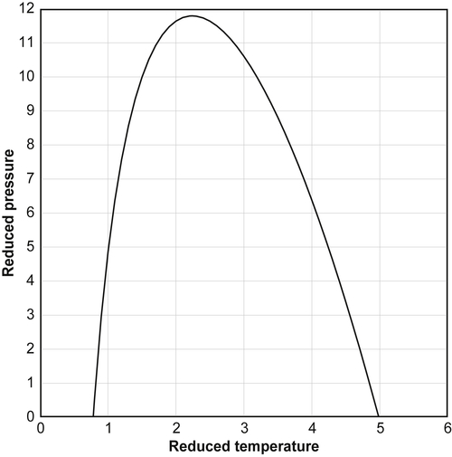
Furthermore, it appears from this figure that, in the limit, as the pressure goes to zero, the ideal gas behavior is not exhibited. That is, at low pressure, the Joule–Thomson coefficient is not zero, which was demonstrated earlier, is the case for ideal gases. However, the Miller equation and the figure derived from it says nothing of the magnitude of the Joule–Thomson coefficient. Low-pressure gases have Joule–Thomson coefficients that are small in magnitude and, thus, for practical purposes, are zero.
11.5. Slurry Flow
A slurry is a heterogeneous mixture of an insoluble solid and a fluid (usually a liquid). Slurries are often used to transport a solid compound, such as coal, in a mixture with a liquid, water, or oil. Some discussion of the flow of hydrate slurries was presented earlier in this book, but additional comments are presented here.
In horizontal slurry flow, there are four flow regimes: (1) homogeneous flow, (2) heterogeneous flow, (3) saltation flow, and (4) flow with a stationary bed (Turian and Yuan, 1977).
In homogeneous flow, the slurry flows almost as a single phase with no separation into either phases or layers. This occurs when the settling velocity of the particles is small in comparison with the velocity of the fluid.
If the particles are somewhat larger or if the settling velocity of the particles is larger, then vertical gradients in the particle concentration can occur. This is the heterogeneous flow regime.
If the settling velocities become too large, then the particles with start to settle. The initial settling is the saltation regime. This regime is intermittent, with leaping movement of particles. Typically, the solids are transported by two mechanisms: bulk movement of the particle bed and movement with the fluid above the bed. To visualize this, imagine wind blowing sand off the top of a sand dune.
In the stationary bed regime, the particles have settled to the bottom of the pipeline. This is similar to the bedding of hydrates described below. In this case, the particles will only flow if they are swept along with the fluid flow.
The criteria for determining the flow regime is a function of the drag coefficient, the solids concentration, the velocity, the pipe diameter, the particle size, and the ratio of the densities. Different pressure drop correlations were developed for each flow regime.
In the slurries studied by Turian and Yuan (1977), there was no tendency for the particles to adhere. For example, in a coal-water or a coal-oil slurry, the coal will not agglomerate into a large mass. However, this is indeed the case with hydrates, thus, for hydrate slurries.
In addition, in typical slurries, the solid phase is denser than the liquid. For natural gas hydrates, if the liquid phase is water, then the hydrates are most likely less denser than the water, and will have some buoyancy and will not likely settle to the bottom of the pipe. If the fluid phase is a condensate or an oil, typical density less than 800 kg/m3, then the hydrate will be of greater density, more like the traditional slurry.
11.6. Hydrate Formation in the Reservoir during Production
As a gas flow from the reservoir into the region of the wellbore, the gas expands. If there is no heat transfer with the surrounding formations, then this is an isenthalpic process.
The flow of the gas through the reservoir is governed by Darcy's law (or nearly so). For the radial flow of a gas, Darcy's law is (Smith, 1990):
 (11.9)
where Q is the volumetric flow rate, k is the permeability, h is the thickness of the formation, P is the pressure, μ is the viscosity of the fluid, z is the compressibility factor (z-factor), Tf is the temperature of the fluid, and r is the radial distance. This equation is derived by integrating between two arbitrary points. One must be very careful with the units when using this equation. For American Engineering Units, this equation becomes:
 (11.10)
where Q is in ft3[std]/d, k is in Darcy, h is in ft, P is in psia, μ is centipoise, z is unitless, Tf is in Rankin, and r is in ft.
Furthermore, when this equation was integrated, it was assumed that the properties of the fluid do not change significantly with the changes in the pressure and temperature of the fluid.
11.7. Flow in the Well
The gas from the reservoir enters the wellbore and travels upward. There are two significant factors in determining the pressure drop in the well flow: (1) friction pressure drop and (2) hydrostatic head. In the case of upward flow, both of these effects tend to reduce the pressure of the flowing gas. Smith (1990) provides a procedure for estimating the pressure and temperature in both shut-in and flowing gas wells.
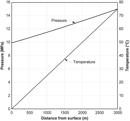
In addition, moving from a depth to the surface, the surrounding temperature decreases the so-called geothermal gradient. Typically, the geothermal gradient is approximately 25 °C/km (1.5 °F/1000 ft).
Fig. 11.3 shows the pressure and temperature as a function of the depth for a hypothetical gas well. The well has a depth of 3000 m (9842 ft) and the pressure at the bottom of the well is 15 MPa (2176 psia), which includes some pressure drop because of the flow through the reservoir. The temperature at 3000 m is 75 °C (167 °F) and the geothermal gradient is 25 °C/km.
Fig. 11.4 shows the same data but on a pressure-temperature plot. Also shown on this graph is the hydrate curve for this gas mixture. It can be seen that the pressure-temperature curve intersects the hydrate curve, which means a hydrate can form in the wellbore. The intersection of the two curves is at approximately 19 °C (66 °F), which is equivalent to a depth of about 750 m (2460 ft). From the surface to about 750 m, hydrate formation is possible in this well. For depths greater than 750 m, the pressure-temperature of the gas is outside the hydrate region and freezing will not occur at greater depths.

In this situation, the injection of an inhibitor chemical is required. Some wells are completed with an injection string that allows for the injection of chemicals at the bottom of the well. This injection is typically continuously preventing production interruption because of plugging of the wellbore. Other wells have a pump at the surface for the injection of chemicals. Unlike pipelines, which are more or less horizontal, the injected chemical can flow down the well string, even if the flow is blocked, because of gravity.
11.8. Carbon Storage
Carbon dioxide has been implemented in global climate change. The capture of carbon dioxide from flue gas and its storage in porous subsurface reservoirs has been touted as a way to reduce anthropogenic CO2 in the atmosphere.
A number of depleted gas reservoirs located in northern Alberta, Canada, and elsewhere, have pressure and temperature conditions that are identified as potential sites for CO2 storage in gas hydrate form. These reservoirs are in the range of pressure from 2 to 5 MPa (290–725 psia) and temperatures from 1° to 10 °C (34°–50 °F). The CO2 must flow into the reservoir for a sufficient distance and then solidify into a hydrate. If the gas solidifies in the wellbore region, the flow would be impeded.
This technology is very new and has only been studied in the laboratory and in simulation (Linga et al., 2009; Zatsepina and Pooladi-Darvish, 2012).
11.9. Transportation
Another potential application of hydrates is for the transportation of natural gas. Currently, gas is transported across continents via pipelines (and there are a few intercontinental pipelines) and via liquid natural gas tankers over longer distances.
For long distance transmission lines, pressures are typically 1000 psia or about 7 MPa. In addition to the pipeline, this involves compression of the gas and, depending upon the distance of the line, may require intermediate recompression.
Transportation of liquid natural gas (LNG) is done at very low temperature but at near atmospheric pressures. It is expensive to liquefy natural gas and requires a vaporization facility at the delivery point.
The industrialization of the transportation of natural gas in the form of hydrates is in its infancy, with several problems that still must be worked out. However, this is not a new idea. Amongst the first to suggest this technology were Cahn et al. (1970).
One of the problems with this method is to produce a hydrate with minimal entrained water, ice (which contains no gas), and a high hydrate concentration. Gudmundsson (1996) describes one possible method for making hydrates on a large scale.
Table 11.1 gives a comparison of the amount of methane contained in 1 m3 (35.3 ft3) of hydrate, 1 m3 of pipeline gas, and 1 m3 (35.3 ft3) of LNG. All of the values are for pure methane and the densities of methane are taken from Wagner and de Reuck (1996). One cubic meter of hydrate contains more than twice as much methane as the pipeline gas, but only about one-fourth of the methane in LNG.
Table 11.1
The Amount of Methane per Cubic Meter for Hydrate, Pipeline Gas, and Liquid
| Pressure (MPa) | Temperature (°C) | Amount (kg) | Comment | |
| Hydrate | 2.6 | 0 | 115 | 1 m3 hydrate contains 170 Sm3 of gas |
| Pipeline gas | 7 | 27 | 50 | Typical pipeline conditions |
| Liquid | 0.101 | −161 | 422 | At the normal boiling point |

| Pressure (psia) | Temperature (°F) | Amount (lb) | Comment | |
| Hydrate | 377 | 32 | 254 | 1 ft3 hydrate contains 170 SCF of gas |
| Pipeline gas | 1015 | 81 | 110 | Typical pipeline conditions |
| Liquid | 14.7 | −258 | 930 | At the normal boiling point |
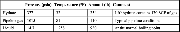
lb, pounds; SCF, standard cubic feet.
11.10. Natural Occurrence of Hydrates
Combinations of water and hydrate formers are common in nature, so it should come as no surprise that there are natural occurrences of gas hydrates. This section reviews them briefly.
11.11. Seabed
There has been much discussion about the occurrence of methane hydrates in the seabed. As was shown in Example 2-7, hydrates of methane can form in the sea at depths of about 300 m (1000 ft). The methane required for the hydrate formation presumably comes from the anaerobic decay of organic material, but may come from other sources.
These hydrates are found throughout the world and not only in colder locations. For example, hydrates have been found in the Gulf of Mexico, the Caribbean Sea, off the cost of South America, India, and many other locations.
Estimates of how much hydrocarbon is locked in these resources are astronomical. For example, Dickens et al. (1997) estimated that there is about 15 GT7 equivalent of methane in the seabed tied up as natural gas hydrates. This is approximately equivalent to 3 × 10¹³ m3[std] or 1 × 10⁹ MMSCF of methane. However, such estimates range widely depending upon who is doing the estimate and what is their basis. For example, Kvenvolden (1999) estimates this amount of gas in seabed hydrates as between 1 × 10¹⁵ and 50 × 1015 m3[std]. Lerche (2001) provides an interesting analysis of the estimates of the hydrate resource.
Others, such as Laherrere (1999), argue that the hydrates are of poor quality and may not be of commercial quality.
11.11.1. Nankai Trough
The Nankai Trough is on the southeast coast of Japan. It is a seismically active area and well known for being rich in seabed hydrates (Colwell et al., 2004). Because they do not have significant convention hydrocarbon reserves, the Japanese are keen to exploit these resources.
According to the Japan Oil, Gas, and Metals National Corporation (JOGMEC), there are 40 TCF of methane in the trough.
In March 2013, JOGMEC announced that it had completed a successful production test (http://www.jogmec.go.jp/english/news/release/) from the Nankai Trough. The test lasted approximately 6 days and resulted in a total of 120 × 103 m3, which is an average of 20 × 103 m3/d. They do not provide much detail other than to say that the production was achieved by depressurization. The gas produced was flared and no processing of the gas was attempted. There was no indication of the pressure or temperature at which the gas arrived at the surface. JOGMEC is hoping for commercial production by the year 2018.
11.12. Natural Gas Formations
In certain cold regions on earth, hydrates can be found in natural gas reservoirs. These include the arctic regions of Canada, Russia, and Alaska.
The production of the gas locked in the hydrates of such a reservoir is an interesting problem. Perhaps a thermal recover method, such as those used for heavy oil, could be used to melt the hydrate. Alternatively, perhaps a miscible flood of an inhibitor chemical could unlock the gas. There have been several papers discussing the production of natural gas from hydrate reservoirs by depressurization. One such paper is by Jia et al. (2001).
11.12.1. Messoyakha Field
An interesting example of a hydrate reservoir is the Messoyakha field in Siberia. This is a natural gas reservoir in a cold region of the world. The field was discovered in 1967 and has been exploited commercially with production from this field that began in 1970. The reservoir had about 850 BCF of natural gas, some of which is frozen in the hydrate.
The gas composition is 98.6% methane, 0.1% ethane, 0.1% C3+, 0.5% carbon dioxide, and 0.7% nitrogen.
The top of the reservoir is at a depth of slightly more than 700 m and the porous formation extends to about 900 m. At approximately 800 m, the pressure and temperature intersect the hydrate curve for the gas in this reservoir. Therefore, there is a free gas zone on the top of the reservoir and a hydrate layer on the bottom.
Gas can be produced from the free gas zone in the top. As this gas is produced, the pressure in the reservoir falls. The reduction in the pressure melts the hydrate releasing additional gas and, thus, increasing the pressure.
More details about this field can be found in Tanahashi (1996) and Makogon et al. (2007).
11.12.2. Mallik
A joint research project lead by the Canadian Geological Survey has thoroughly studied a hydrate formation in the delta of the Mackenzie River in the Canadian Arctic (north of the Arctic Circle).
The drilled a well to a depth of about 1150 m (3770 ft) where hydrates were encountered in a sandstone formation. The formation is about 100 m (325 ft) thick. It is estimated that the structure contains about 100 × 109 m3 of gas frozen in the hydrate. As of the writing of this book, this resource has not been exploited commercially.
There are many papers discussing this project, but a good summary is given by Hyndman and Dallimore (2001).
11.13. Outer Space
The frigid conditions in outer space along with the possibility of water make for the potential of hydrates in outer space. Two examples are provided here.
11.13.1. Comets
Miller (1961) was among the first to speculate on the possibility of hydrates in outer space. It is ironic that, at the time of his paper, it was commonly believed that there were no natural hydrates on the Earth. In fact, Miller (1961) begins his paper by stating:
The gas hydrates… are not known to occur naturally on the earth because of the unfavorable combination of temperatures, pressures, and gases that are poor hydrate formers.
It seems to be well known that comets are stellar “ice balls.” However, comets are a witch's brew of water and organic compounds. These are the right combination for hydrate formation. Miller was among the first to speculate upon this possibility.
11.13.2. Mars
The Martian atmosphere is approximately 95.3% CO2, 2.7% nitrogen, 1.6% argon, and the remainder (less than half of 1%) is oxygen, carbon monoxide, and others. The atmospheric pressure on the surface of Mars is 0.636 mbars. This data comes from the Website www.burro.astr.cwru.edu.
Water is also known to exist on Mars and there are prominent “ice caps” on both the south and north poles.
Much like the Earth, there are large variations in the temperature on the surface of Mars because of time of the Martian day, Martian seasons, and latitude. However, at the poles in the Martian winter, the temperature can be as low as 120 K (−153 °C).
Miller and Smythe (1970) speculated on the possibility of hydrates in the “ice” caps on Mars. They concluded that because Martian atmosphere contains carbon dioxide and if the “ice” caps contain water, there is a possibility that hydrates can be formed.
In January 1999, National Aeronautics and Space Administration launched the Mars Polar Lander (MPL) with the intention of exploring the south pole of Mars. It had the equipment to determine whether the ice cap was composed of hydrate or ice. Unfortunately, communication was lost with the spacecraft in December 1999 and it was never recovered. Therefore, the MPL is essentially “lost in space.” Thus, an answer based on measurements from Mars will have to wait for another mission. For more details see: http://mars.jpl.nasa.gov/msp98/lander/.
In addition, the gas giant planets in our solar system: Saturn, Jupiter, and Neptune, and their moons, contain methane and water. Surely, there is a possibility that hydrates exist on those planets as well.
Examples
Example 11.1
Pure methane is throttled from 51.85 °C (325 K) and 5–3.5 MPa. The calculations for the exit temperature were made using the methane tables from Wagner and de Reuck (1996).
Answer: From the tables:
| 5 MPa | 320 K | 91.416 J/mol | |
| 330 K | 501.42 J/mol | ||
| Interpolating enthalpy | 325 K | 296.42 J/mol |

From the tables:
| 3.5 MPa | 320 K | 301.82 J/mol | |
| 310 K | −93.104 J/mol | ||
| Interpolating temperature | 319.42 K | 296.42 J/mol |

Therefore, the outlet temperature is 319.42 K or 46.71 °C. Therefore, the temperature drop is 5.14 °C. From this, the Joule–Thomson coefficient can be approximated:

Example 11.2
For the information given below, calculate the gas flow rate through the reservoir.
| k = 0.005 Darcy | h = 50 ft |
| μ = 0.0175 cp | z = 0.925 |
| Tf = 120 °F = 580 R | |
| r2 = 2640 ft | r1 = 0.25 ft |
| P2 = 3000 psia | P1 = 1000 psia |
Answer: Substituting into the Darcy equation and performing the arithmetic:

Example 11.3
Assuming the gas in the previous example is pure methane, estimate the temperature drop due to the expansion using the tables from Wagner and de Reuck (1996).
Answer: The tables are in SI units so the original pressures are converted from psia to MPa:
Convert from AEU to SI units:

Double interpolate the table to get the value of the enthalpy at the initial conditions:
| Pressure (MPa) | Temperature (K) | Enthalpy (J/mol) | Comments |
| 13 | 320 | −979.79 | From tables |
| 13 | 330 | −493.33 | From tables |
| 13 | 322.04 | −880.55 | Interpolated |
| 14 | 320 | −604.60 | From tables |
| 14 | 330 | −118.81 | From tables |
| 14 | 322.04 | −505.50 | Interpolated |
| 13.789 | 322.04 | −584.64 | Interpolated |

Because this is a constant enthalpy process, the enthalpy at the initial condition is equal to the enthalpy at the final conditions. Thus, find the temperature at 6.985 MPa and −584.64 J/mol.
| Pressure (MPa) | Temperature (K) | Enthalpy (J/mol) | Comments |
| 6.5 | 300 | −974.38 | From tables |
| 6.5 | 310 | −544.57 | From tables |
| 6.5 | 309.07 | −584.64 | Interpolated |
| 7 | 310 | −619.62 | From tables |
| 7 | 320 | −187.80 | From tables |
| 7 | 310.81 | −584.64 | Interpolated |
| 6.895 | 310.57 | −584.64 | Interpolated |

Therefore, the estimated temperature is 310.57 K, which is equal to 37.4 °C or 99.4 °F. Thus, the expansion of the gas as it flows from the bulk reservoir (120 °F) to the wellbore has resulted in a cooling of about 20 °F.
This is an overly simple analysis and did not account for the changes in the properties because of the change in the temperature in the original Darcy's law calculation.
..................Content has been hidden....................
You can't read the all page of ebook, please click here login for view all page.