
Chapter 2
Data Mining Process
Abstract
Successfully uncovering patterns using data mining is an iterative process. Chapter 2 provides a framework to solve the data mining problem. The five-step process outlined in this chapter provides guidelines on gathering subject matter expertise; exploring the data with statistics and visualization; building a model using data mining algorithms; testing the model and deploying it in a production environment; and finally reflecting on new knowledge gained in the cycle. Over the years of evolution of data mining practices, different frameworks for the data mining process have been put forward by various academic and commercial bodies, like the Cross Industry Standard Process for Data Mining, knowledge discovery in databases, etc. These data mining frameworks exhibit common characteristics and hence we will be using a generic framework closely resembling the CRISP process.
Keywords
CRISP; KDD; data mining process; prior knowledge; modeling; data preparation; evaluation; applicationThe methodological discovery of useful relationships and patterns in data is enabled by a set of iterative activities known as data mining process. The standard data mining process involves (1) understanding the problem, (2) preparing the data samples, (3) developing the model, (4) applying the model on a data set to see how the model may work in real world, and (5) production deployment. Over the years of evolution of data mining practices, different frameworks for the data mining process have been put forward by various academic and commercial bodies. In this chapter, we will discuss the key steps involved in building a successful data mining solution. The framework we put forward in this chapter is synthesized from a few data mining frameworks, and is explained using a simple example data set. This chapter serves as a high-level roadmap in building deployable data mining models, and discusses the challenges faced in each step, as well as important considerations and pitfalls to avoid. Most of the concepts discussed in this chapter are reviewed later in the book with detailed explanations and examples.
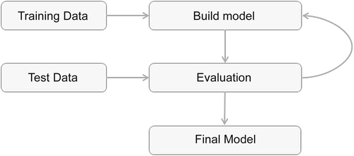
One of the most popular data mining process frameworks is CRISP-DM, which is an acronym for Cross Industry Standard Process for Data Mining. This framework was developed by a consortium of many companies involved in data mining (Chapman et al., 2000). The CRISP-DM process is the most widely adopted framework for developing data mining solutions. Figure 2.1 provides a visual overview of the CRISP-DM framework. Other data mining frameworks are SEMMA, which is an acronym for Sample, Explore, Modify, Model, and Assess, developed by the SAS Institute (SAS Institute, 2013); DMAIC, which is an acronym for Define, Measure, Analyze, Improve and Control, used in Six Sigma practice (Kubiak & Benbow, 2005); and the Selection, Preprocessing, Transformation, Data Mining, Interpretation, and Evaluation framework used in the knowledge discovery in databases (KDD) process (Fayyad et al., 1996). We feel all these frameworks exhibit common characteristics and hence we will be using a generic framework closely resembling the CRISP process. As with any process framework, a data mining process recommends the performance of a certain set of tasks to achieve optimal output. The process of extracting information from the data is iterative. The steps within the data mining process are not linear and have many loops, going back and forth between steps and at times going back to the first step to redefine data mining problem statement.

The data mining process presented in Figure 2.2 is a generic set of steps that is business, algorithm, and, data mining tool agnostic. The fundamental objective of any process that involves data mining is to address the analysis question. The problem at hand could be segmentation of customers or predicting climate patterns or a simple data exploration. The algorithm used to solve the business question could be automated clustering or an artificial neural network. The software tools to develop and implement the data mining algorithm used could be custom coding, IBM SPSS, SAS, R, or RapidMiner, to mention a few.
Data mining, specifically in the context of big data, has gained a lot of importance in the last few years. Perhaps the most visible and discussed part of data mining is the third step: modeling. It involves building representative models that can be derived from the sample data set and can be used for either predictions (predictive modeling) or for describing the underlying pattern in the data (descriptive or explanatory modeling). Rightfully so, there is plenty of academic and business research in this step and we have dedicated most of the book to discussing various algorithms and quantitative foundations that go with it. We specifically wish to emphasize considering data mining as an end-to-end, multistep, iterative process instead of just a model building step. Seasoned data mining practitioners can attest to the fact that the most time-consuming part of the overall data mining process is not the model building part, but the preparation of data, followed by data and business understanding. There are many data mining tools, both open source and commercial, available in the market that can automate the model building. The most commonly used tools are RapidMiner, R, Weka, SAS, SPSS, Oracle Data Miner, Salford, Statistica, etc. (Piatetsky, 2014). Asking the right business questions, gaining in-depth business understanding, sourcing and preparing the data for the data mining task, mitigating implementation considerations, and, most useful of all, gaining knowledge from the data mining process, remains crucial to the success of the data mining process. Lets get started with Step 1: Framing the data mining question and understanding the context.

2.1. Prior Knowledge
Prior knowledge refers to information that is already known about a subject. The objective of data mining doesn’t emerge in isolation; it always develops on top of existing subject matter and contextual information that is already known. The prior knowledge step in the data mining process helps to define what problem we are solving, how it fits in the business context, and what data we need to solve the problem.
2.1.1. Objective
The data mining process starts with an analysis need, a question or a business objective. This is possibly the most important step in the data mining process (Shearer, 2000). Without a well-defined statement of the problem, it is impossible to come up with the right data set and pick the right data mining algorithm. Even though the data mining process is a sequential process and it is common to go back to previous steps and revise the assumptions, approach, and tactics. It is imperative to get the objective of the whole process right, even if it is exploratory data mining.
We are going to explain the data mining process using an hypothetical example. Let’s assume we are in the consumer loan business, where a loan is provisioned for individuals with the collateral of assets like a home or car, i.e., a mortgage or an auto loan. As many home owners know, an important component of the loan, for the borrower and the lender, is the interest rate at which the borrower repays the loan on top of the principal. The interest rate on a loan depends on a gamut of variables like the current federal funds rate as determined by the central bank, borrower’s credit score, income level, home value, initial deposit (down payment) amount, current assets and liabilities of the borrower, etc. The key factor here is whether the lender sees enough reward (interest on the loan) for the risk of losing the principal (borrower’s default on the loan). In an individual case, the status of default of a loan is Boolean; either one defaults or not, during the period of the loan. But, in a group of tens of thousands of borrowers, we can find the default rate—a continuous numeric variable that indicates the percentage of borrowers who default on their loans. All the variables related to the borrower like credit score, income, current liabilities, etc. are used to assess the default risk in a related group; based on this, the interest rate is determined for a loan. The business objective of this hypothetical use case is: If we know the interest rate of past borrowers with a range of credit scores, can we predict interest rate for a new borrower?
2.1.2. Subject Area
The process of data mining uncovers hidden patterns in the data set by exposing relationships between attributes. But the issue is that it uncovers a lot of patterns. False signals are a major problem in the process. It is up to the data mining practitioner to filter through the patterns and accept the ones that are valid and relevant to answer the objective question. Hence, it is essential to know the subject matter, the context, and the business process generating the data.
The lending business is one of the oldest, most prevalent, and complex of all the businesses. If the data mining objective is to predict the interest rate, then it is important to know how the lending business works, why the prediction matters, what we do once we know the predicted interest rate, what data points can be collected from borrowers, what data points cannot be collected because of regulations, what other external factors can affect the interest rate, how we verify the validity of the outcome, and so forth. Understanding current models and business practices lays the foundation and establishes known knowledge. Analysis and mining the data provides the new knowledge that can be built on top of existing knowledge (Lidwell et al., 2003).
2.1.3. Data
Similar to prior knowledge in the subject area, there also exists prior knowledge in data. Data is usually collected as part of business processes in a typical enterprise. Understanding how the data is collected, stored, transformed, reported, and used is essential for the data mining process. This part of the step considers all the data available to answer the business question and if needed, what data needs to be sourced from the data sources. There are quite a range of factors to consider: quality of the data, quantity of data, availability of data, what happens when data is not available, does lack of data compel the practitioner to change the business question, etc. The objective of this step is to come up with a data set, the mining of which answers the business question(s). It is critical to recognize that a model is only as good as the data used to create it.
For the lending example, we have put together an artificial data set of ten data points with three attributes: identifier, credit score, and interest rate. First, let’s look at some of the terminology used in the data mining process in relation to describing the data.
▪ A data set (example set) is a collection of data with a defined structure. Table 2.1 shows a data set. It has a well-defined structure with 10 rows and 3 columns along with the column headers.
▪ A data point (record or data object or example) is a single instance in the data set. Each row in Table 2.1 is a data point. Each instance contains the same structure as the data set.
▪ An attribute (feature or input or dimension or variable or predictor) is a single property of the data set. Each column in Table 2.1 is an attribute. Attributes can be numeric, categorical, date-time, text, or Boolean data types. In this example, credit score and interest rate are numeric attribute.
▪ A label (class label or output or prediction or target or response) is the special attribute that needs to be predicted based on all input attributes. In Table 2.1, interest rate is the output variable.
▪ Identifiers are special attributes that are used for locating or providing context to individual records. For example, common attributes like Names, account numbers, employee ID are identifier attributes. Identifiers are often used as lookup keys to combine multiple data sets. They bear no information that is suitable for building data mining models and should thus be excluded for the actual modeling step. In Table 2.1, the ID is the identifier.
2.1.4. Causation vs. Correlation
Let’s invert our prediction objective: Based on the data in Table 2.1, can we predict the credit score of the borrower based on interest rate? The answer is yes—but it doesn’t make business sense. From existing domain expertise, we know credit score influences the loan interest rate. Predicting credit score based on interest rate inverses that causation relationship. This question also exposes one of the key aspects of model building. The correlation between the input and output attributes doesn’t guarantee causation. Hence, it is very important to frame the data mining question correctly using the existing domain and data knowledge. In this data mining example, we are going to predict the interest rate of the new borrower with unknown interest rate (Table 2.2) based on the pattern learned from known data in Table 2.1.
2.2. Data Preparation
Preparing the data set to suit a data mining task is the most time-consuming part of the process. Very rarely data are available in the form required by the data mining algorithms. Most of the data mining algorithms would require data to be structured in a tabular format with records in rows and attributes in columns. If the data is in any other format, then we would need to transform the data by applying pivot or transpose functions, for example, to condition the data into required structure. What if there are incorrect data? Or missing values? For example, in hospital health records, if the height field of a patient is shown as 1.7 centimeters, then the data is obviously wrong. For some records height may not be captured in the first place and left blank. Following are some of the activities performed in Data Preparation stage, along with common challenges and mitigation strategies.
2.2.1. Data Exploration
Data preparation starts with an in-depth exploration of the data and gaining more understanding of the data set. Data exploration, also known as Exploratory Data Analysis (EDA), provides a set of simple tools to achieve basic understanding of the data. Basic exploration approaches involve computing descriptive statistics and visualization of data. Basic exploration can expose the structure of the data, the distribution of the values, the presence of extreme values and highlights the interrelationships within the data set. Descriptive statistics like mean, median, mode, standard deviation, and range for each attribute provide an easily readable summary of the key characteristics of the distribution of the data. On the other hand, a visual plot of data points provides an instant grasp of all the data points condensed into one chart. Figure 2.3 shows the scatterplot of credit score vs. loan interest rate and we can observe that as credit score increases, interest rate decreases. We will review more data exploration techniques in Chapter 3. In general, a data set sourced to answer a business question has to be analyzed, prepared, and transformed before applying algorithms and creating models.

2.2.2. Data Quality
Data quality is an ongoing concern wherever data is collected, processed, and stored. In the data set used as an example (Table 2.1), how do we know if the credit score and interest rate data are accurate? What if a credit score has a recorded value of 900 (beyond the theoretical limit) or if there was a data entry error? These errors in data will impact the representativeness of the model. Organizations use data cleansing and transformation techniques to improve and manage the quality of data and store them in companywide repositories called Data Warehouses. Data sourced from well-maintained data warehouses have higher quality, as there are proper controls in place to ensure a level of data accuracy for new and existing data. The data cleansing practices include elimination of duplicate records, quarantining outlier records that exceed the bounds, standardization of attribute values, substitution of missing values, etc. Regardless, it is critical to check the data using data exploration techniques in addition to using prior knowledge of the data and business before building models to ensure a certain degree of data quality.
2.2.3. Missing Values
One of the most common data quality issues is that some records having missing attribute values. For example, a credit score may be missing in one of the records. There are several different mitigation methods to deal with this problem, but each method has pros and cons. The first step in managing missing values is to understand the reason behind why the values are missing. Tracking the data lineage of the data source can lead to identifying systemic issues in data capture, errors in data transformation, or there may be a phenomenon that is not understood to the user yet. Knowing the source of a missing value will often guide what mitigation methodology to use. We can substitute the missing value with a range of artificial data so that we can manage the issue with marginal impact on the later steps in data mining. Missing credit score values can be replaced with a credit score derived from the data set (mean or minimum or maximum value, depending on the characteristics of the attribute). This method is useful if the missing values occur completely randomly and the frequency of occurrence is quite rare. If not, the distribution of the attribute that has missing data will be distorted. Alternatively, to build the representative model, we can ignore all the data records with missing value or records with poor data quality. This method reduces the size of the data set. Some data mining algorithms are good at handling records with missing values, while others expect the data preparation step to handle it before model is built and applied. For example, k-nearest neighbor (k-NN) algorithm for classification tasks are often robust with missing values. Neural network models for classification tasks do not perform well with missing attributes and thus the data preparation step is essential for developing neural network models.
2.2.4. Data Types and Conversion
The attributes in a data set can be of different types, such as continuous numeric (interest rate), integer numeric (credit score), or categorical. In some data sets, credit score is expressed as ordinal or categorical (poor, good, excellent). Different data mining algorithms impose different restrictions on what data types they accept as inputs. If the model we are about to build is a simple linear regression model, the input attributes need to be numeric. If the data that is available is categorical, then it needs to be converted to continuous numeric attribute. There are several methods available for conversion of categorical types to numeric attributes. For instance, we can encode a specific numeric score for each category value, such as poor = 400,good = 600, excellent = 700, etc. Similarly, numeric values can be converted to categorical data types by a technique called binning, where a range of values are specified for each category, e.g, low = [400–500] and so on.
2.2.5. Transformation
In some data mining algorithms like k-NN, the input attributes are expected to be numeric and normalized, because the algorithm compares the values of different attributes and calculates distance between the data points. It is important to make sure one particular attribute doesn’t dominate the distance results because of large values or because it is denominated in smaller units. For example, consider income (expressed in USD, in thousands) and credit score (in hundreds). The distance calculation will always be dominated by slight variation in income. One solution is to convert the range of income and credit score to a more uniform scale from 0 to 1 by standardization or normalization. This way, we can make a consistent comparison between the two different attributes with different units. However, the presence of outliers may potentially skew the results of normalization.
In a few data mining tasks, it is necessary to reduce the number of attributes. Statistical techniques like principal component analysis (PCA) reduce attributes into a few key or principal attributes. PCA is discussed in Chapter 12 Feature Selection. The presence of multiple attributes that are highly correlated may be undesirable for few algorithms. For example, having both annual income and taxes paid are highly correlated and hence we may need to remove one of the attributes. This is explained in a little more detail in Chapter 5 Regression Methods, where we discuss regression.
2.2.6. Outliers
Outliers by definition are anomalies in the data set. Outliers may occur legitimately (income in billions) or erroneously (human height 1.73 centimeters). Regardless, the presence of outliers needs to be understood and will require special treatment. The purpose of creating a representative model is to generalize a pattern or a relationship in the data and the presence of outliers skews the model. The techniques for detecting outliers will be discussed in detail in Chapter 11 Anomaly Detection on anomaly detection. Detecting outliers may be the primary purpose of some data mining applications, like fraud detection and intrusion detection.
2.2.7. Feature Selection
The example data set shown in Table 2.1 has one attribute or feature—credit score—and one label—interest rate. In practice, many data mining problems involve a data set with hundreds to thousands of attributes. In text mining applications (see Chapter 9 Text Mining), every distinct word in a document is considered an attribute in the data set. Thus the data set used in this application contains thousands of attributes. Not all the attributes are equally important or useful in predicting the desired target value. Some of the attributes may be highly correlated with each other, like annual income and taxes paid. The presence of a high number of attributes in the data set significantly increases the complexity of a model and may degrade the performance of the model due to the curse of dimensionality. In general, the presence of more detailed information is desired in data mining because discovering nuggets of a pattern in the data is one of the attractions of using data mining techniques. But, as the number of dimensions in the data increases, data becomes sparse in high-dimensional space. This condition degrades the reliability of the models, especially in the case of clustering and classification (Tan et al., 2005).
Reducing the number of attributes, without significant loss in the performance of the model, is called feature selection. Chapter 12 provides details on different techniques available for feature selection and its implementation considerations. Reducing the number of attributes in the data set leads to a more simplified model and helps to synthesize a more effective explanation of the model.
2.2.8. Data Sampling
Sampling is a process of selecting a subset as a representation of the original data set for use in data analysis or modeling. Sample data serves as a representative of the original data set with similar properties, such as a similar mean. Sampling reduces the amount of data that needs to be processed for analysis and modeling. In most cases, to gain insights, extract the information and build representative predictive models from the data it is sufficient to work with samples. Sampling speeds up the build process of the modeling. Theoretically, the error introduced by sampling impacts the relevancy of the model but their benefits far outweighs the risks.
In the build process for Predictive Analytics applications, it is necessary to segment the data sets to training and test samples. Depending on the application, the training data set is sampled from the original data set using simple sampling or class label specific sampling. Let us consider the use cases for predicting anomalies in a data. Depending on the application, the training data set is sampled from the original data set using simple sampling or class label specific sampling. Let us consider the use cases for predicting anomalies in a data set (e.g., predicting fraudulent credit card transactions).
The objective of anomaly detection is to classify outliers in the data. These are rare events and often the example data does not have many examples of the outlier class. Stratified sampling is a process of sampling where each class is equally represented in the sample; this allows the model to focus on the difference between the patterns of each class. In classification applications, sampling is used create multiple base models, each developed using a different set of sampled training data sets. These base models are using to build one meta model, called the ensemble model, where the error rate is improved when compared to that of the base models.
2.3. Modeling
A model is the abstract representation of the data and its relationships in a given data set. A simple statement like “mortgage interest rate reduces with increase in credit score” is a model; although there is not enough quantitative information to use in a production scenario, it provides directional information to abstract a relationship between credit score and interest rate.
There are a few hundred data mining algorithms in use today, derived from statistics, machine learning, pattern recognition, and computer science body of knowledge. Fortunately, there are many viable commercial and open source predictive analytics and data mining tools in the market that implement these algorithms. As a data mining practitioner, all we need to be concerned with is having an overview of the algorithm. We want to know how it works and determine what parameters need to be configured based on our understanding of the business and data. Data mining models can be classified into the following categories: classification, regression, association analysis, clustering, and outlier or anomaly detection. Each category has a few dozen different algorithms; each takes a slightly different approach to solve the problem at hand. Classification and regression tasks are predictive techniques because they predict an outcome variable based on one or more input variables. Predictive algorithms need a known prior data set to “learn” the model. Figure 2.4 shows the steps in the modeling phase of predictive data mining. Association analysis and clustering are descriptive data mining techniques where there is no target variable to predict; hence there is no test data set. However, both predictive and descriptive models have an evaluation step. Anomaly detection can be predictive if known data is available or use unsupervised techniques if the known training data is not available.
2.3.1. Training and Testing Data Sets
To develop a stable model, we need to make use of a previously prepared data set where we know all the attributes, including the target class attribute. This is called the training data set and it is used to create a model. We also need to check the validity of the created model with another known data set called the test data set or validation data set. To facilitate this process, the overall known data set can be split into a training data set and a test data set. A standard rule of thumb is for two-thirds of the data to go to training and one-third to go to the test data set. There are more sophisticated approaches where training records are selected by random sampling with replacement, which we will discuss in Chapter 4 Classification. Tables 2.3 and 2.4 show the random split of training and test data, based on the example data set shown in Table 2.1. Figure 2.5 shows the scatterplot of the entire example data set with the training and test data sets marked.
2.3.2. Algorithm or Modeling Technique
The business question and data availability dictate what data mining category (association, classification, regression, etc.) needs to be used. The data mining practitioner determines the appropriate data mining algorithm within the chosen category. For example, within classification any of the following algorithms can be chosen: decision trees, rule induction, neural networks, Bayesian models, k-NN, etc. Likewise within decision tree techniques, there are quite a number of implementations like CART, RAID, etc. We will review all these algorithms in detail in later chapters. It is not uncommon to use multiple data mining categories and algorithms to solve a business question.
Interest rate prediction is considered a regression problem. We are going to use a simple linear regression technique to model the data set and generalize the relationship between credit score and interest rate. The data set with 10 records can be split into training and test sets. The training set of seven records will be used to create the model and the test set of three records will be used to evaluate the validity of the model.

The objective of simple linear regression can be visualized as fitting a straight line through the data points in a scatterplot (Figure 2.6). The line has to be built in such a way that the sum of the squared distance from the data points to the line is minimal. Generically, the line can be expressed as
![]() (2.1)
(2.1)
where y is the output or dependent variable, x is the input or independent variable, b is the y-intercept, and a is the coefficient of x. We can find the values of a and b in such a way so as to minimize the sum of the squared residuals of the line (Weisstein, 2013). We will review the concepts and steps in developing a linear regression model in greater detail in Chapter 5 Regression Methods.
The line shown in Equation 2.1 serves as a model to predict the outcome of new unlabeled data set. For the interest rate data set, we have calculated the simple linear regression for the interest rate (y):
![]()

![]()
Using this model we can calculate the interest rate for a specified credit score of the borrower. Linear regression is one of the simplest models to get us started in model building and more complex models are discussed later in this book. In reality, the rate calculation involves a few dozen input variables and also takes into account the nonlinear relationship between variables.
2.3.3. Evaluation of the Model
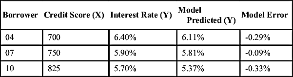
The model generated in the form of an equation is generalized and synthesized from seven training records. We can substitute the credit score in the equation and see if the model estimates the interest rate for each of the seven training records. The estimation may not be exactly the same as the values in the training records. We do not want a model to memorize and output the same values that are in the training records. The phenomenon of a model memorizing the training data is called overfitting, which will be explored in Chapter 4 Classification. An overfitted model just memorizes the training records and will underperform on real production data. We want the model to generalize or learn the relationship between credit score and interest rate. To evaluate this relationship, the validation or test data set, which was not previously used in building the model, is used for evaluation, as shown in Table 2.5.
Table 2.5 provides the three testing records where the interest rate is known; these records were not used to build the model. The actual value of the interest rate can be compared against the predicted value using the model and thus the prediction error can be calculated. As long as the error is acceptable, this model can be used for deployment. The error rate can be used to compare this model with other models developed from different algorithms like neural networks or Bayesian models, etc.
2.3.4. Ensemble Modeling
Ensemble modeling is a process where multiple diverse models are created to predict an outcome, either by using many different modeling algorithms or using different training data sets. The ensemble model then aggregates the prediction of each base model and results in once final prediction for the unseen data. The motivation for using ensemble models is to reduce the generalization error of the prediction. As long as the base models are diverse and independent, the prediction error of the model decreases when the ensemble approach is used. The approach seeks the wisdom of crowds in making a prediction. Even though the ensemble model has multiple base models within the model, it acts and performs as a single model. Most of the practical data mining solutions utilize ensemble modeling techniques. Chapter 4 Classification covers the approaches of different ensemble modeling techniques and their implementation in detail.
At the end of the modeling stage of the data mining process, we have (1) analyzed the business question, (2) sourced the data relevant to answer the question, (3) picked a data mining technique to answer the question, (4) picked a data mining algorithm and prepared the data to suit the algorithm, (5) split the data into training and test data sets, (6) built a generalized model from the training data set, and (7) validated the model against the test data set. This model now can be used to predict the target variable based on an input variable of unseen data. This answers the business question on prediction. Now, the model needs to be deployed, for example by integrating the model in the production loan approval process of an enterprise.
2.4. Application
Deployment or application is the stage at which the model becomes production ready or “live.” In business applications, the results of the data mining, either the model for predictive tasks or the learning framework for association rules or clustering, need to be assimilated into the business process—usually in software applications. The model deployment stage leads to some key considerations: assessing model readiness, technical integration, response time, model maintenance, and assimilation.
2.4.1. Production Readiness
The production readiness part of the deployment determines the critical qualities required for the deployment objective. Let’s consider two distinct use cases: determining whether a consumer qualifies for a loan account with a commercial leading institution and determining the groupings of customers for an enterprise.
The consumer credit approval process is a real-time endeavor. Either through a consumer-facing website or through a specialized application for frontline agents, the credit decisions and terms need to be provided in real time as soon as prospective customers provide relevant information. It is seen as a competitive advantage to provide a quick decision while also providing accurate results in the interest of customer and the company. The decision-making model needs to collect data from the customer, integrate third-party data like credit history, and make a decision on the loan approval and terms in a matter of seconds. The critical quality in this model deployment is real-time prediction.
Segmenting customers based on their relationship with the company is a thoughtful process where signals from various interactions through a number of departments in a company are considered. Based on the patterns, similar customers are put in cohorts and treatment strategies are deviced to best engage the customer. For this application, batch processing, where data is collected overnight from various departments and sources, is integrated and the overall customer records are segmented. The critical quality in this application is the ability to find unique patterns amongst customers, not the response time of the model. The business application informs the choices that need to be made in data preparation and modeling steps, in terms of accessibility of the data and algorithms.
2.4.2. Technical Integration
Most likely some kind of data mining software tool (R, RapidMiner, SAS, SPSS, etc.) would have been used to create the data mining models. Data mining tools save time by not requiring the writing of custom codes to implement the algorithm. This allows the analyst to focus on the data, business logic, and exploring patterns from the data. The models created by data mining tools can be ported to production applications by utilizing the Predictive Model Markup Language (PMML) (Guazzelli et al., 2009) or by invoking data mining tools in the production application. PMML provides a portable and consistent format of model description which can be read by most Predictive Analytics and Data Mining tools. This allows the flexibility for practitioners to develop the model with one tool (e.g., RapidMiner) and deploy it in another tool (e.g., SAS). PMML standards are developed and maintained by the Data Mining Group, an industry-lead consortium. Models such as simple regression, decision trees, and induction rules for predictive analytics can be incorporated directly into business applications and business intelligence systems easily. Since these models are represented by simple equations and if-then rules, they can be ported easily to most programming languages.
2.4.3. Response Time
Some data mining algorithms, like k-NN, are easy to build but quite slow in predicting the target variables. Algorithms such as the decision tree take time to build but can be reduced to simple rules that can be coded into almost any application. The trade-offs between production responsiveness and build time need to be considered and if needed, the modeling phase needs to be revisited if the response time is not acceptable by business application. The quality of prediction, accessibility of input data and the response time of the prediction remains the most important quality factors in the business application.
2.4.4. Remodeling
The key criterion for the ongoing relevance of the model is the representativeness of the data set it is processing. It is quite normal that the conditions in which the model is built change after the model is sent to deployment. For example, the relationship between the credit score and interest rate change frequently based on the prevailing macroeconomic conditions. Hence the model needs to be updated frequently for this application. The validity of the model can be routinely tested by using the new known test data set and calculating the error rate. If the error rate exceeds a particular threshold, then we can rebuild the model and redo the deployment. Creating a maintence schedule is a key part of a deployment plan that will sustain a living model.
2.4.5. Assimilation
In descriptive data mining applications, deploying a model to live systems may not be the objective. The challenge is often to assimilate the knowledge gained from data mining to the organization or a specific application. For example, the objective may be finding logical clusters in the customer database so that separate treatment can be provided to each customer cluster. Then the next step may be a classification task for new customers to put them in one of known clusters. Association analysis provides a solution for the market basket problem, where the task is to find which two products are purchased together most often. The challenge for the data mining practitioner is to articulate these findings, relevance to the original business question, a quantification of risks in the model and expected business impact to the business users. Often, this is a challenging task for data mining practitioner. The business user community is an amalgamation of different point of views, different quantitative mind set and skill set. Not everyone is aware about process of Data Mining and what it can and cannot do. Some aspect of this challenge can be addressed by focusing on the end result and it’s impact of knowing the information instead of technical process of extracting the information through data mining. Understanding and rationalizing the results for these tasks may lead to taking action through business processes.
2.5. Knowledge
The data mining process provides a framework to extract nontrivial information from data. With the advent of massive storage, increased data collection, and advanced computing paradigms, the data at our disposal are only increasing. To extract knowledge from these massive data assets, we need to employ advanced approaches like data mining algorithms, in addition to standard time series reporting or simple statistical processing. Though many of these algorithms can provide valuable knowledge extraction, it’s up to the analytics professional to skillfully apply the right algorithms and transform a business problem to a data problem. Data mining, like any other technology, provides options in terms of algorithms and parameters within the algorithms. Using these options to extract the right information is a bit of art and can be developed with practice.
The data mining process starts with prior knowledge and ends with posterior knowledge, which is the incremental insight gained about the business via data through the process. As with any quantitative analysis, the data mining process can point out spurious irrelevant patterns from the data set. Not all discovered patterns leads to knowledge. Again, it is upon the practitioner to invalidate the irrelevant patterns and identify meaningful information. The impact of the information gained through data mining can be measured in an application. It’s the difference between having the information through the data mining process and the insights from basic data analysis. Finally, the whole data mining process is a framework to invoke the right questions (Chapman et al., 2000) and guide us through the right approaches to solve a business problem. It is not meant to be used as a set of rigid rules, but as a set of iterative, distinct steps that aid in knowledge discovery.
What’s Next?
In upcoming chapters, we will dive into the details of the concepts discussed in this chapter, along with the implementation details. Exploring data by using basic statistical and visual techniques are an important step in preparing the data for data mining. The next chapter on Data Exploration provides a practical tool kit to explore and understand the data. The techniques of data preparation are explained in the context of individual data mining techniques in the chapters on classification, association analysis, clustering, and anomaly detection. Chapter 13 Getting Started with RapidMiner covers the practical implementation of data preparation techniques using RapidMiner.
..................Content has been hidden....................
You can't read the all page of ebook, please click here login for view all page.