
Chapter 12
Feature Selection
Abstract
This chapter introduces a preprocessing step that is critical for a successful predictive modeling exercise: feature selection. Feature selection is known by several alternative terms such as attribute weighting, dimension reduction, and so on. There are two main styles of feature selection: filtering the key attributes before modeling (filter style) or selecting the attributes during the process of modeling (wrapper style). We discuss a few filter-based methods such as PCA, information gain, and chi-square, and a couple of wrapper-type methods like forward selection and backward elimination.
Keywords
Attribute weighting; backward elimination; chi-square test; dimension reduction; feature selection; filter type; forward selection; information gain; PCA; wrapper typeIn this chapter we will focus on an important component of data set preparation for predictive analytics: feature selection. An overused rubric in data mining circles is that 80% of the analysis effort is spent on data cleaning and preparation and only 20% is typically spent on modeling. In light of this it may seem strange that this book has devoted more than a dozen chapters to modeling techniques and only a couple to data preparation! However, data cleansing and preparation are things that are better learned through experience and not so much from a book. That said, it is essential to be conversant with the many techniques that are available for these important early process steps. We are not going to be focusing on data cleaning in this chapter, which was partially covered in Chapter 2 Data Mining Process but on reducing a data set to its essential characteristics or features. This process goes by various terms: feature selection, dimension reduction, variable screening, key parameter identification, attribute weighting. (Technically, there is a subtle difference between dimension reduction and feature selection. Dimension reduction methods—such as principal component analysis, discussed in Section 12.2—combine or merge actual attributes in order to reduce the number of attributes of a raw data set. Feature selection methods work more like filters that eliminate some attributes.)
We start out with a brief introduction to feature selection and the need for this preprocessing step. There are fundamentally two types of feature selection processes: filter type and wrapper type. Filter approaches work by selecting only those attributes that rank among the top in meeting certain stated criteria (Blum, 1997; Yu, 2003). Wrapper approaches work by iteratively selecting, via a feedback loop, only those attributes that improve the performance of an algorithm. (Kohavi, 1997) Among the filter-type methods, we can classify further based on the data types: numeric versus nominal. The most common wrapper-type methods are the ones associated with multiple regression: stepwise regression, forward selection, and backward elimination. We will explore a few numeric filter-type methods: principal component analysis (PCA), which is strictly speaking a dimension reduction method; information gain–based filtering; and one categorical filter-type method: chi-square-based filtering. We will briefly discuss, using a RapidMiner implementation, the two wrapper-type methods.
12.1. Classifying Feature Selection Methods
There are two powerful technical motivations for incorporating feature selection in the data mining process. Firstly, a data set may contain highly correlated attributes, such as the number of items sold and the revenue earned by the sales of the item. We are typically not gaining any new information by including both of these attributes. Additionally, in the case of multiple regression–type models, if two or more of the independent variables (or predictors) are correlated, then the estimates of coefficients in a regression model tend to be unstable or counter intuitive. This is the multicollinearity discussed in Section 5.1. In the case of algorithms like naïve Bayesian classifiers, the attributes need to be independent of each other. Further, the speed of algorithms is typically a function of the number of attributes. So by using only one among the correlated attributes we improve the performance.
Secondly, a data set may also contain redundant information that does not directly impact the predictions: as an extreme example, a customer ID number has no bearing on the amount of revenue earned from the customer. Such attributes may be filtered out by the analyst before the modeling process may begin. However, not all attribute relationships are that clearly known in advance. In such cases, we must resort to computational methods to detect and eliminate attributes that add no new information. The key here is to include attributes that have a strong correlation with the predicted or dependent variable.
So, to summarize, feature selection is needed to remove independent variables that may be strongly correlated to one another, and to make sure we keep independent variables that may be strongly correlated to the predicted or dependent variable.
We may apply feature selection methods before we start the modeling process and filter out unimportant attributes or we may apply feature selection methods iteratively within the flow of the data mining process. Depending upon the logic, we have two feature selection schemes: filter schemes or wrapper schemes. The filter scheme does not require any learning algorithm, whereas the wrapper type is optimized for a particular learning algorithm. In other words, the filter scheme can be considered “unsupervised” and the wrapper scheme can be considered a “supervised” feature selection method. The filter model is commonly used in the following scenarios:
▪ When the number of features or attributes is really large
▪ When computational expense is a criterion
The chart in Figure 12.1 summarizes a high level taxonomy of feature selection methods, some of which we will explore in the following sections, as indicated. This is not meant to be a comprehensive taxonomy, but simply a useful depiction of the techniques commonly employed in data mining and described in this chapter.
12.2. Principal Component Analysis
We will start with a conceptual introduction to PCA before showing the mathematical basis behind the computation. We will then demonstrate how to apply PCA to a sample data set using RapidMiner.

Let us assume that we have a dataset with m attributes (or variables). These could be for example, commodity prices, weekly sales figures, number of hours spent by assembly line workers, etc.; in short any business parameter that can have an impact on a performance that is captured by a label or target variable. The question that PCA helps us to answer fundamentally is this: Which of these m attributes explain a significant amount of variation contained within the data set? PCA essentially helps to apply an 80/20 rule: Can a small subset of attributes (the 20%) explain 80% or more of the variation in the data? This sort of variable screening or feature selection will make it easy to apply other predictive modeling techniques and also make the job of interpreting the results easier.
PCA captures the attributes that contain the greatest amount of variability in the data set. It does this by transforming the existing variables into a set of “principal components” or new variables that have the following properties (van der Maaten et al., 2009):
▪ They are uncorrelated with each other.
▪ They cumulatively contain/explain a large amount of variance within the data.
▪ They can be related back to the original variables via weightage factors.
The original variables with very low weightage factors in their principal components are effectively removed from the data set. The conceptual schematic in Figure 12.2 illustrates how PCA can help in reducing data dimensions with a hypothetical dataset of m variables.

12.2.1. How it Works
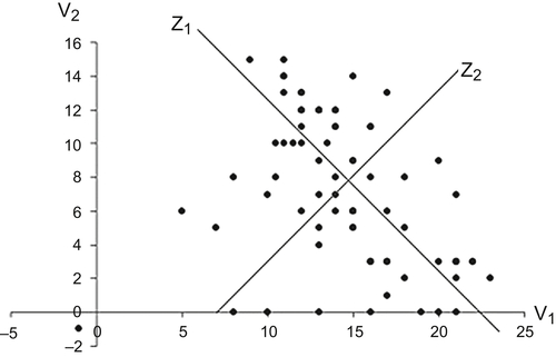
The key task is computing the principal components, zm, which have the properties that were described just above. Consider the case of just two variables: v1 and v2. When the variables are visualized using a scatterplot, we would see something like the one shown in Figure 12.3.
As can be seen, v1 and v2 are correlated. But we could transform v1 and v2 into two new variables z1 and z2, which meet our guidelines for principal components, by a simple linear transformation. As seen in the chart, this amounts to plotting the points along two new axes: z1 and z2. Axis z1 contains the maximum variability, and one can rightly conclude that z1 explains a significant majority of the variation present in the data and is the first principal component. z2, by virtue of being orthogonal to z1, contains the next highest amount of variability. Between z1 and z2 we can account for (in this case of two variables) 100% of the total variability in the data. Furthermore, z1 and z2 are uncorrelated. As we increase the number of variables, vm, we may find that only the first few principal components are sufficient to express all the data variances. The principal components, zm, are expressed as a linear combination of the underlying variables, vm:
![]() (12.1)
(12.1)
When we extend this logic to more than two variables, the challenge is to find the transformed set of principal components using the original variables. This is easily accomplished by performing an eigenvalue analysis of the covariance matrix of the original attributes.1 The eigenvector associated with the largest eigenvalue is the first principal component; the eigenvector associated with the second largest eigenvalue is the second principal component and so on. The covariance explains how two variables vary with respect to their corresponding mean values—if both variables tend to stay on the same side of their respective means, the covariance would be positive, if not it would be negative. (In statistics, covariance is also used in the calculation of correlation coefficient.)
![]() (12.2)
(12.2)
where expected value E[v] = vk P(v = vk). For the eigenvalue analysis, a matrix of such covariances between all pairs of variables vm is created. The reader is referred to standard textbooks on matrix methods or linear algebra for more details behind the eigenvalue analysis (Yu, 2003).
12.2.2. How to Implement
In this section, we will start with a publicly available data set2 and use RapidMiner to perform the PCA. Furthermore, for illustrative reasons, we will work with nonstandardized or nonnormalized data. In the next part we will standardize the data and explain why it may be important sometimes to do so.
The data set includes information on ratings and nutritional information on 77 breakfast cereals. There are a total of 16 variables, including 13 numerical parameters (Table 12.1). The objective is to reduce this set of 13 numerical predictors to a much smaller list using PCA.
Step 1: Data Preparation
Remove the nonnumeric parameters “Cereal name,” “Manufacturer,” and “Type (hot or cold),” because PCA can only work with numeric attributes. These are columns A, B, and C. (In RapidMiner, we can convert these into ID attributes if needed for reference later. This can be done during the import of the data set into RapidMiner during the next step if needed; in this case we will simply remove these variables. The Select Attributes operator may also be used following the Read Excel operator to remove these variables.)
Table 12.1
Breakfast cereals data set for dimension reduction using PCA
| name | mfr | type | calories | protein | fat | sodium | fiber | carbo | sugars | potass | vitamins | shelf | weight | cups | rating |
| 100%_Bran | N | C | 70 | 4 | 1 | 130 | 10 | 5 | 6 | 280 | 25 | 3 | 1 | 0.33 | 68.402973 |
| 100%_Natural_Bran | Q | C | 120 | 3 | 5 | 15 | 2 | 8 | 8 | 135 | 0 | 3 | 1 | 1 | 33.983679 |
| All-Bran | K | C | 70 | 4 | 1 | 260 | 9 | 7 | 5 | 320 | 25 | 3 | 1 | 0.33 | 59.425505 |
| All-Bran_with_Extra_Fiber | K | C | 50 | 4 | 0 | 140 | 14 | 8 | 0 | 330 | 25 | 3 | 1 | 0.5 | 93.704912 |
| Almond_Delight | R | C | 110 | 2 | 2 | 200 | 1 | 14 | 8 | -1 | 25 | 3 | 1 | 0.75 | 34.384843 |
| Apple_Cinnamon_Cheerios | G | C | 110 | 2 | 2 | 180 | 1.5 | 10.5 | 10 | 70 | 25 | 1 | 1 | 0.75 | 29.509541 |
| Apple_Jacks | K | C | 110 | 2 | 0 | 125 | 1 | 11 | 14 | 30 | 25 | 2 | 1 | 1 | 33.174094 |
| Basic_4 | G | C | 130 | 3 | 2 | 210 | 2 | 18 | 8 | 100 | 25 | 3 | 1.33 | 0.75 | 37.038562 |

Read the Excel file into RapidMiner: this can be done using the standard Read Excel operator as described in earlier sections.
Step 2: PCA Operator
Type in the keyword “pca” in the operator search field and drag and drop the Principal Component Analysis operator into the main process window. Connect the output of Read Excel into the “Example set input” or “exa” port of the PCA operator.
The three available parameter settings for dimensionality reduction are none, keep variance, and fixed number. Here we use keep variance and leave the variance threshold at the default value of 0.95 or 95% (see Figure 12.4). The variance threshold selects only those attributes that collectively account for or explain 95% (or any other value set by user) of the total variance in the data. Connect all output ports from the PCA operator to the results ports.
Step 3: Execution and Interpretation
By running the analysis as configured above, RapidMiner will output several tabs in the results panel (Figure 12.5). By clicking on the PCA tab, we will see three PCA related tabs—Eigenvalues, Eigenvectors, and Cumulative Variance Plot.
Using Eigenvalues, we can obtain information about the contribution to the data variance coming from each principal component individually and cumulatively.
If, for example, our variance threshold is 95%, then PC 1, PC 2, and PC 3 are the only principal components that we need to consider because they are sufficient to explain nearly 97% of the variance. PC 1 contributes to a majority of this variance, at about 54%.
We can then “deep dive” into these three components and identify how they are linearly related to the actual or real parameters from the data set. At this point we consider only those real parameters that have significant weightage contribution to the each of the first three PCs. These will ultimately form the subset of reduced parameters for further predictive modeling.


The key question is how do we select the real variables based on this information? RapidMiner allows us to sort the eigenvectors (weighting factors) for each PC and we can decide to choose the two to three highest (absolute) valued weighting factors for PCs 1 to 3. As seen from Figure 12.6, we have chosen the highlighted real attributes—calories, sodium, potassium, vitamins, and rating—to form the reduced data set. This selection was done by simply identifying the top three attributes from each principal component.3
For the above example, PCA reduces the number of attributes from 13 to 5, a more than 50% reduction in the number of attributes that any model would need to realistically consider. One can imagine the improvement in performance as we deal with the larger data sets that PCA enables. In practice, PCA is a very effective and widely used tool for dimension reduction, particularly when all attributes are numeric. It works for a variety of real-world applications, but it should not be blindly applied for variable screening. For most practical situations, domain knowledge should be used in addition to PCA analysis before eliminating any of the variables. Here are some observations that explain some of the risks to consider while using PCA.

1. The results of a PCA must be evaluated in the context of the data.
If the data is extremely noisy, then PCA may end up suggesting that the noisiest variables are the most significant because they account for most of the variation!
An analogy would be the total sound energy in a rock concert. If the crowd noise drowns out some of the high-frequency vocals or notes, PCA might suggest that the most significant contribution to the total energy comes from the crowd—and it will be right! But this does not add any clear value if one is attempting to distinguish which musical instruments are influencing the harmonics, for example.
2. Adding uncorrelated data does not always help. Neither does adding data that may be correlated, but irrelevant.
When we add more parameters to our data set, and if these parameters happen to be random noise, we are effectively led back to the same situation as the first point above. On the other hand, as analysts we also have to exercise caution and watch out for spurious correlations. As an extreme example, it may so happen that there is a correlation between the number of hours worked in a garment factory and pork prices (an unrelated commodity) within a certain period of time. Clearly this correlation is probably pure coincidence. Such correlations again can muddy the results of a PCA. Care must be taken to winnow the data set to include variables that make business sense and are not subjected to many random fluctuations before applying a technique like tPCA.

3. PCA is very sensitive to scaling effects in the data.
If we examine the data in the above example closely, we will see that the top attributes that PCA helped identify as the most important ones also have the widest range (and standard deviation) in their values. For example, potassium ranges from –1 to 330 and sodium ranges from 1 to 320. Comparatively, most of the other factors range in the single or low double digits. As expected, these factors dominate PCA results because they contribute to the maximum variance in the data. What if there was another factor such as sales volume, which would potentially range in the millions (of dollars or boxes), were to be considered for a modeling exercise? Clearly it would mask the effects of any other attribute.
To minimize scaling effects, we can range normalize the data (using for example, the Normalize operator). When we apply this data transformation, all attributes are reduced to a range between 0 and 1 and scale effects will not matter anymore. But what happens to the PCA results?
As Figure 12.7 shows, we now need eight PCs to account for the same 95% total variance. As an exercise, you can use the eigenvectors to filter out the attributes that are included in these eight PCs and you will find that (applying the top three rule for each PC as before), you have not eliminated any of the attributes!
This brings us to the next section on feature selection methods that are not scale sensitive and also work with nonnumerical datasets, which were two of the limitations with PCA.
12.3. Information Theory–Based Filtering for Numeric Data
In Chapter 4 we encountered the concepts of information gain and gain ratio. Recall that both of these methods involve comparing the information exchanged between a given attribute and the target or label attribute (Peng et al., 2005). As we discussed in Section 12.1, the key to feature selection is to include attributes that have a strong correlation with the predicted or dependent variable. With these techniques, we can rank attributes based on the amount of information gain and then select only those that meet or exceed some (arbitrarily) chosen threshold or simply select the top k (again, arbitrarily chosen) features.
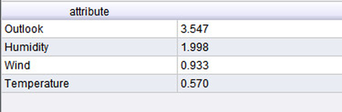
Let us revisit the golf example we discussed first in Chapter 4. The data is presented here again for convenience in Figure 12.8a. When we apply the information gain calculation methodology that was discussed in Chapter 4 to compute information gain for all attributes (see Table 4.2), we will arrive at the feature ranking in Figure 12.8b in terms of their respective “influence” on the target variable “Play.” This can be easily done using the Weight by Information Gain operator in RapidMiner. The output looks almost identical to the one shown in Table 4.2, except for the slight differences in the information gain values for Temperature and Humidity. The reason is that for that data set, we had converted the temperature and humidity into nominal values before computing the gains. In this case, we use the numeric attributes as they are. So it is important to pay attention to the discretization of the attributes before filtering. Use of information gain feature selection is also restricted to cases where the label is nominal. For fully numeric datasets, where the label variable is also numeric, PCA or correlation-based filtering methods are commonly used.
Figure 12.9 describes a process that uses the sample Golf data set available in RapidMiner. The various steps in the process convert numeric attributes, Temperature and Humidity, into nominal ones. In the final step, we apply the Weight by Information Gain operator to both the original data and converted data set in order to show the difference between the gain computed using different data types. The main point to observe is that the gain computation depends not only upon the data types, but also how the nominal data is discretized. For example, we get slightly different gain values (see Table 12.2) if we divide Humidity into three bands (high, medium, and low) as opposed to only two bands (high and low). The reader can test these variants very easily using the process described. In conclusion, we select the top-ranked attributes. In this case, they would be Outlook and Temperature if we choose the nondiscretized version, and Outlook and Humidity in the discretized version.


12.4. Chi-Square-Based Filtering for Categorical Data
In many cases our data sets may consist of only categorical (or nominal) attributes. In this case, what is a good way to distinguish between high influence attributes and low or no influence attributes?
A classic example of this scenario is the gender selection bias. Suppose we have data about the purchase of a big-ticket item like a car or a house. Can we verify the influence of gender on purchase decisions? Are men or women the primary decision makers when it comes to purchasing big-ticket items? For example, is gender a factor in color preference of a car? Here attribute 1 would be gender and attribute 2 would be the color. A chi-square test would reveal if there is indeed a relationship between these two attributes. If we have several attributes and wish to rank the relative influence of each of these on the target attribute, we can still use the chi-square statistic.

Let us go back to the golf example in Figure 12.10—this time we have converted all numeric attributes into nominal ones. Chi-square analysis involves counting occurrences (of number of sunny days or windy days) and comparing these variables to the target variable based on the frequencies of occurrences. The chi-square test checks if the frequencies of occurrences across any pair of attributes, such as Outlook = overcast and Play = yes, are correlated. In other words, for the given Outlook type, overcast, what is the probability that Play = yes (existence of a strong correlation)? The multiplication law of probabilities states that if event A happening is independent of event B, then the probabilities of A and B happening together is simply pA ∗ pB. The next step is to convert this joint probability into an “expected frequency,” which is given by pA ∗ pB ∗ N, where N is the sum of all occurrences in the data set.
For each attribute, a table of observed frequencies, such as the one shown in Table 12.3, is built. This is called a contingency table. The last column and row (the margins) are simply the sums in the corresponding rows or columns as you can verify. Using the contingency table, a corresponding expected frequency table can be built using the expected frequency definition (pA ∗ pB ∗N) from which the chi-square statistic is then computed by comparing the difference between the observed frequency and expected frequency for each attribute. The expected frequency table for Outlook is shown in Table 12.4.
The expected frequency for the event [Play = no and Outlook= sunny] is calculated using our expected frequency formula as (5/14 ∗ 5/14 ∗14) =1.785 and is entered in the first cell as shown. Similarly, the other expected frequencies are calculated. The formula for the chi-square statistic is the summation of the square of the differences between observed and expected frequencies, as given in Equation 12.2:
![]() (12.2)
(12.2)
where fo is the observed frequency and fe is the expected frequency. The test of independence between any two parameters is done by checking if the observed chi-square is less than a critical value that depends upon the confidence level chosen by the user (Black, 2007). In this case of feature weighting, we simply gather all the observed chi-square values and use them to rank the attributes. The ranking of attributes for our golf example is generated using the process described in Figure 12.11 and is shown in the table of observed chi-square values in Figure 12.12. Just like in information gain feature selection, most of the operators shown in the process are simply transforming the data into nominal values to generate it in the form shown in Figure 12.10.
Compare the output of the chi-square ranking to the information gain–based ranking (for the nominalized or discretized attributes) and you will see that the ranking is identical.


Note that the “Normalize weights” option is sometimes also used, which is a range normalization onto the interval 0 to 1.
12.5. Wrapper-Type Feature Selection
In this section of the chapter we will briefly introduce wrapper scheme feature reduction methods by using a linear regression example. As explained earlier, the wrapper approach iteratively chooses features to add or to remove from the current attribute pool based on whether the newly added or removed attribute improves the accuracy.
Wrapper-type methods originated from the need to reduce the number of attributes that are needed to build a high-quality regression model. A very thorough way to build regression models is something called the “all possible regressions” search procedure. For example, with thre attributes, v1, v2, and v3, we could build the different regression models in Table 12.5.
In general, if a data set contains k different attributes, then conducting all possible regression searches implies that we build 2k – 1 separate regression models and pick the one that has the best performance. Clearly this is impractical.
A better way, from a computational resource consumption point of view, to do this search would be to start with one variable, say v1, and build a baseline model. Then add a second variable, say v2, and build a new model to compare with the baseline. If the performance of the new model, for example, the R2 (see Chapter 5), is better than that of the baseline, we make this model the new baseline, add a third variable, v3, and proceed in a similar fashion. If however, the addition of the second attribute, v2, did not improve the model significantly (over some arbitrarily prescribed level of improvement in performance), then we pick a new attribute v3, and build a new model that includes v1 and v3. If this model is better than the model that included v1 and v2, we proceed to the next step, where we will consider a next attribute v4, and build a model that includes v1, v3, and v4. In this way, we step forward selecting attributes one by one until we achieve a desired level of model performance. This process is called forward selection.4
A reverse of this process is where we start our baseline model with all the attributes, v1, v2, …, vk and for the first iteration, remove one of the variables, vj, and construct a new model. However, how do we select which vj to remove? Here, it is typical to start with a variable that has the lowest t-stat value, as you will see in the following case study.5 If the new model is better than the baseline, it becomes the new baseline and the search continues to remove variables with the lowest t-stat values until some stopping criterion is met (usually if the model performance is not significantly improved over the previous iteration). This process is called backward elimination.
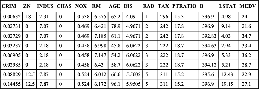
As you can see, the variable selection process wraps around the modeling procedure, hence the name for these classes of feature selection. We will now examine a case study, using data from the Boston Housing6 model first introduced in Chapter 5, to demonstrate how to implement the backward elimination method using RapidMiner. You may recall that the data consists of 13 predictors and 1 response variable. The predictors include physical characteristics of the house (such as number of rooms, age, tax, and location) and neighborhood features (school, industries, zoning), among others. The response variable is the median value (MEDV) of the house in thousands of dollars. These 13 independent attributes are considered to be predictors for the target or label attribute. The snapshot of the data table is shown again in Table 12.6 for continuity.
12.5.1. Backward Elimination to Reduce the Data Set
Our goal here is to build a high-quality multiple regression model that includes as few attributes as possible, without compromising the predictive ability of the model.
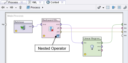
The logic used by RapidMiner for applying these techniques is not “linear,” but a nested logic. The graphic in Figure 12.13 explains how this nesting was used in setting up the training and testing of the Linear Regression operator for the analysis we did in Chapter 5 on the Boston Housing data. The arrow indicates that the training and testing process was nested within the Split Validation operator.
In order to apply a wrapper-style feature selection method such as backward elimination, we need to tuck the training and testing process inside another subprocess, a learning process. The learning process is now nested inside the Backward Elimination operator. We therefore now have double nesting as schematically shown in Figure 12.13. Next, Figure 12.14 shows how to configure the Backward Elimination operator in RapidMiner. Double clicking on the Backward Elimination operator opens up the learning process ,which can now accept the Split Validation operator we have used many times.

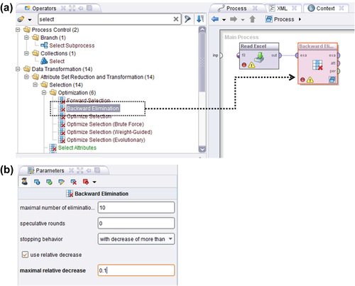
Table 12.6
Sample view of the Boston Housing data set
| CRIM | ZN | INDUS | CHAS | NOX | RM | AGE | DIS | RAD | TAX | PTRATIO | B | LSTAT | MEDV |
| 0.00632 | 18 | 2.31 | 0 | 0.538 | 6.575 | 65.2 | 4.09 | 1 | 296 | 15.3 | 396.9 | 4.98 | 24 |
| 0.02731 | 0 | 7.07 | 0 | 0.469 | 6.421 | 78.9 | 4.9671 | 2 | 242 | 17.8 | 396.9 | 9.14 | 21.6 |
| 0.02729 | 0 | 7.07 | 0 | 0.469 | 7.185 | 61.1 | 4.9671 | 2 | 242 | 17.8 | 392.83 | 4.03 | 34.7 |
| 0.03237 | 0 | 2.18 | 0 | 0.458 | 6.998 | 45.8 | 6.0622 | 3 | 222 | 18.7 | 394.63 | 2.94 | 33.4 |
| 0.06905 | 0 | 2.18 | 0 | 0.458 | 7.147 | 54.2 | 6.0622 | 3 | 222 | 18.7 | 396.9 | 5.33 | 36.2 |
| 0.02985 | 0 | 2.18 | 0 | 0.458 | 6.43 | 58.7 | 6.0622 | 3 | 222 | 18.7 | 394.12 | 5.21 | 28.7 |
| 0.08829 | 12.5 | 7.87 | 0 | 0.524 | 6.012 | 66.6 | 5.5605 | 5 | 311 | 15.2 | 395.6 | 12.43 | 22.9 |
| 0.14455 | 12.5 | 7.87 | 0 | 0.524 | 6.172 | 96.1 | 5.9505 | 5 | 311 | 15.2 | 396.9 | 19.15 | 27.1 |
The Backward Elimination operator can now be filled in with the Split Validation operator and all the other operators and connections required to build a regression model. The process of setting these up is exactly the same as discussed in Chapter 5 and hence is not repeated here. Now let us look at the configuration of the Backward Elimination operator. Here we can specify several parameters to enable feature selection. The most important one is the “stopping behavior.” Our choices are “with decrease,” “with decrease of more than,” and “with significant decrease.” The first choice is very parsimonious—a decrease from one iteration to the next will stop the process. But if we pick the second choice, we have to now indicate a “maximal relative decrease.” In this example, we have indicated a 10% decrease. Finally, the third choice is very stringent and requires achieving some desired statistical significance by allowing you to specify an alpha level. But we have not said by how much the performance parameter should decrease yet! This is specified “deep inside” the nesting: all the way at the Performance operator that was selected in the Testing window of the Split Validation operator. In this example, the performance criterion was “squared correlation.” For a complete description of all the other Backward Elimination parameters, the RapidMiner help can be consulted.
There is one more step that may be helpful to complete before running this model. Simply connecting the Backward Elimination operator ports to the output will not show us the final regression model equation. To be able to see that, we need to connect the “exa” port of the Backward Elimination operator to another Linear Regression operator in the main process. The output of this operator will contain the model, which can be examined in the Results perspective. The top level of the final process is shown in Figure 12.15.
12.5.2. What Variables have been Eliminated by Backward Elimination?
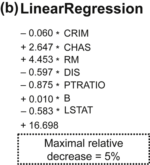
Comparing the two regression equations (Figure 12.16a below and in Chapter 5, see Figure 5.6a) we can see that nine attributes have been eliminated. Perhaps the 10% decrease was too aggressive. As it happens, the R2 for the final model with only three attributes was only 0.678. If we were to change the stopping criterion to a 5% decrease, we will end up with an R2 of 0.812 and now have 8 of the 13 original attributes (Figure 12.16b). You can also see that the regression coefficients for the two models are different as well. The final judgment on what is the right criterion and its level can only be made with experience with the data set and of course, good domain knowledge.
Each iteration using a regression model either removes or introduces a variable, which improves model performance. The iterations stop when a preset stopping criterion or no change in performance criterion (such as adjusted R2 or RMS error) is reached. The inherent advantage of wrapper-type methods are that multicollinearity issues are automatically handled. However, you get no prior knowledge about the actual relationship between the variables. Applying forward selection is very similar and is left as an exercise for the reader.

Conclusion
This chapter covered the basics of a very important part of the overall data mining paradigm: feature selection or dimension reduction. A central hypothesis among all the feature selection methods is that good feature selection results in attributes or features that are highly correlated with the class, yet uncorrelated with each other (Hall, 1999). We presented a high-level classification of feature selection techniques and explored each of them in some detail. As stated at the beginning of this chapter, dimension reduction is best understood with real practice. To this end, we recommend readers apply all the techniques described in the chapter on all the data sets provided. We saw that the same technique can yield quite different results based on the selection of analysis parameters. This is where data visualization can play an important role. Sometimes, examining a correlation plot between the various attributes, like in a scatterplot matrix, can provide valuable clues about which attributes are likely redundant and which ones can be strong predictors of the label variable. While there is usually no substitute for domain knowledge, sometimes data is simply too large or mechanisms are unknown. This is where feature selection can actually help.
..................Content has been hidden....................
You can't read the all page of ebook, please click here login for view all page.