Clustering
Abstract
Clustering is an unsupervised data mining technique where the records in a data set are organized into different logical groupings. The groupings are in such a way that records inside the same group are more similar than records outside the group. Clustering has a wide variety of applications ranging from market segmentation to customer segmentation, electoral grouping, web analytics, and outlier detection. Clustering is also used as a data compression technique and data preprocessing technique for supervised data mining tasks. Many different data mining approaches are available to cluster the data and are developed based on proximity between the records, density in the data set, or novel application of neural networks. K-means clustering, density clustering, and self-organizing map techniques are reviewed in the chapter along with implementations using RapidMiner.
Keywords
Centriod; clustering; DBSCAN; density clustering; k-means clustering; Kohonen networks; Kohonen networks; self-organizing mapsClustering to Describe the Data
Clustering for Preprocessing
7.1. Types of Clustering Techniques


7.2. k-Means Clustering

7.2.1. How it Works: Concepts
Step 1: Initiate Centroids
Step 2: Assign Data Points
![]() (7.1)
(7.1)


Step 3: Calculate New Centroids
 (7.2)
(7.2)
 (7.3)
(7.3)Step 4: Repeat Assignment and Calculate New Centroids
Step 5: Termination
Special Cases

Evaluation of Clusters
7.2.2. How to Implement
Step 1: Data Preparation

Step 2: Clustering Operator and Parameters
Step 3: Evaluation
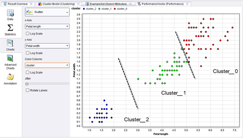
Step 4: Execution and Interpretation


7.3. DBSCAN Clustering
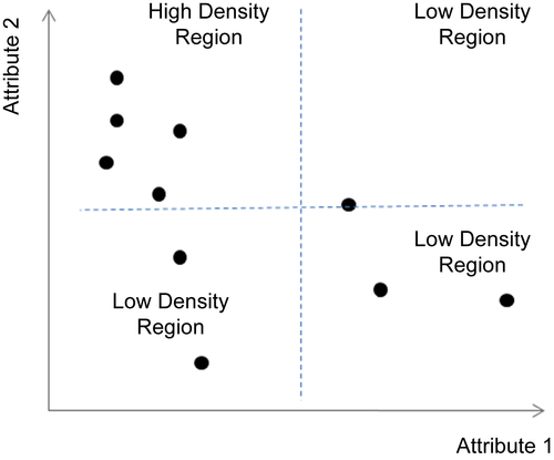

7.3.1. How it Works
Step 1: Defining Epsilon and MinPoints
Step 2: Classification of Data Points

Step 3: Clustering
Optimizing Parameters
Special Cases: Varying Densities


7.3.2. How to Implement
Step 1: Data Preparation
Step 2: Clustering Operator and Parameters
Step 3: Evaluation (Optimal)
Step 4: Execution and Interpretation


7.3.3. Conclusion
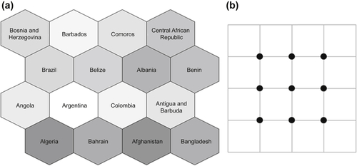
7.4. Self-Organizing Maps
7.4.1. How it Works: Concepts
Step 1: Topology Specification
Step 2: Initialize Centroids
Step 3: Assignment of Data Objects
Step 4: Centroid Update


![]() (7.5)
(7.5)