In classification or class prediction, we try to use the information from the predictors or independent variables to sort the data samples into two or more distinct classes or buckets. Classification is the most widely used data mining task in business. There are several ways to build classification models. In this chapter, we will discuss and show the implementation of six of the most commonly used classification algorithms: decision trees, rule induction, k-nearest neighbors, naïve Bayesian, artificial neural networks, and support vector machines. We conclude this chapter with building ensemble classification models and a discussion on bagging, boosting, and random forests.
Keywords
Classification; decision trees; rule induction; k-nearest neighbors; naïve Bayesian; artificial neural networks; support vector machines; ensemble; bagging; boosting; random forests
We are entering the realm of predictive analytics—the process in which historical records are used to make a prediction about an uncertain future. At a very fundamental level, most predictive analytics problems can be categorized into either classification or numeric prediction problems. In classification or class prediction, we try to use the information from the predictors or independent variables to sort the data samples into two or more distinct classes or buckets. In the case of numeric prediction, we try to predict the numeric value of a dependent variable using the values assumed by the independent variables, as is done in a traditional regression modeling.
Let us describe the classification process with a simple, fun example. Most golfers enjoy playing if the weather and outlook conditions meet certain requirements: too hot or too humid conditions, even if the outlook is sunny, are not preferred. On the other hand, overcast skies are no problem for playing even if the temperatures are somewhat cool. Based on the historic records of these conditions and preferences, and information about a day’s temperature, humidity level, and outlook, classification will allow us to predict if someone prefers to play golf or not. The outcome of classification is to categorize the weather conditions when golf is likely to be played or not, quite simply: Play or Not Play (two classes). The predictors can be continuous (temperature, humidity) or categorical (sunny, cloudy, windy, etc.). Those beginning to explore predictive analytics tools are confused by the dozens of techniques that are available to address these types of classification problems. In this chapter we will explore several commonly used data mining techniques where the idea is to develop rules, relationships, and models based on predictor information that can be applied to classify outcomes from new and unseen data.
We start out with fairly simple schemes and progress to more sophisticated techniques. Each section contains essential algorithmic details about the technique, describes how it is developed using simple examples, and finally closes out with implementation details using RapidMiner.
4.1. Decision Trees
Decision trees (also known as classification trees) are probably one of the most intuitive and frequently used data mining techniques. From an analyst’s point of view, they are easy to set up and from a business user’s point of view they are easy to interpret. Classification trees, as the name implies, are used to separate a data set into classes belonging to the response variable. Usually the response variable has two classes: Yes or No (1 or 0). If the response variable has more than two categories, then variants of the decision tree algorithm have been developed that may be applied (Quinlan, 1986). In either case, classification trees are used when the response or target variable is categorical in nature.
Regression trees (Brieman, 1984) are similar in function to classification trees and may be used for numeric prediction problems, when the response variable is numeric or continuous: for example, predicting the price of a consumer good based on several input factors. Thus regression trees are applicable for prediction type of problems as opposed to classification. Keep in mind that in either case, the predictors or independent variables may be either categorical or numeric. It is the target variable that determines the type of decision tree needed. (Collectively, the algorithm for classification and regression trees is referred to as CART.)
4.1.1. How it Works
A decision tree model takes a form of decision flowchart (or an inverted tree) where an attribute is tested in each node. At end of the decision tree path is a leaf node where a prediction is made about the target variable based on conditions set forth by the decision path. The nodes split the data set into subsets. In a decision tree, the idea is to split the data set based on homogeneity of data. Let us say for example we have two variables, age and weight, that predict if a person is likely to sign up for a gym membership or not. In our training data if it was seen that 90% of the people who are older than 40 signed up, we may split the data into two parts: one part consisting of people older than 40 and the other part consisting of people under 40. The first part is now “90% pure” from the standpoint of which class they belong to. However we need a rigorous measure of impurity, which meets certain criteria, based on computing a proportion of the data that belong to a class. These criteria are simple:
1. The measure of impurity of a data set must be at a maximum when all possible classes are equally represented. In our gym membership example, in the initial data set if 50% of samples belonged to “not signed up” and 50% of samples belonged to “signed up,” then this nonpartitioned raw data would have maximum impurity.
2. The measure of impurity of a data set must be zero when only one class is represented. For example, if we form a group of only those people who signed up for the membership (only one class = members), then this subset has “100% purity” or “0% impurity.”
Measures such as entropy or Gini index easily meet these criteria and are used to build decision trees as described in the following sections. Different criteria will build different trees through different biases, for example, information gain favors tree splits that contain many cases, while information gain ratio attempts to balance this.
How Predictive Analytics can Reduce Uncertainty in a Business Context: The Concept of Entropy
Imagine a box that can contain one of three colored balls inside—red, yellow, and blue, see Figure 4.1. Without opening the box, if you had to “predict” which colored ball is inside, you are basically dealing with lack of information or uncertainty. Now what is the highest number of “yes/no” questions that can be asked to reduce this uncertainty and thus increase our information?
1. Is it red? No.
2. Is it yellow? No.
Then it must be blue.
That is two questions. If there were a fourth color, green, then the highest number of yes/no questions is three. By extending this reasoning, it can be mathematically shown that the maximum number of binary questions needed to reduce uncertainty is essentially log(T), where the log is taken to base 2 and T is the number of possible outcomes (Meagher, 2005) (e.g., if you have only one color, i.e., one outcome, then log(1) = 0, which means there is no uncertainty!)
Many real world business problems can be thought of as extensions to this “uncertainty reduction” example. For example, knowing only a handful of characteristics such as the length of a loan, borrower’s occupation, annual income, and previous credit behavior, we can use several of the available predictive analytics techniques to rank the riskiness of a potential loan, and by extension, the interest rate of the loan. This is nothing but a more sophisticated uncertainty reduction exercise, similar in spirit to the ball-in-a-box problem. Decision trees embody this problem-solving technique by systematically examining the available attributes and their impact on the eventual class or category of a sample. We will examine in detail later in this section how to predict the credit ratings of a bank’s customers using their demographic and other behavioral data and using the decision tree which is a practical implementation of the entropy principle for decision making under uncertainty.
Figure 4.1Playing 20 questions with entropy.
Continuing with the example in the box, if there are T events with equal probability of occurrence P, then T = 1/P. Claude Shannon, who developed the mathematical underpinnings for information theory (Shannon, 1948), defined entropy as log(1/P) or –log P where P is the probability of an event occurring. If the probability for all events is not identical, we need a weighted expression and thus entropy, H, is adjusted as follows:
H=−∑pklog2(pk)
(4.1)
where k = 1, 2, 3, …, m represent the m classes of the target variable. The pk represent the proportion of samples that belong to class k. For our gym membership example from earlier, there are two classes: member or nonmember. If our data set had 100 samples with 50% of each, then the entropy of the dataset is given by H = –[(0.5 log2 0.5) + (0.5 log2 0.5)] = –log2 0.5 = –(–1) = 1. On the other hand, if we can partition the data into two sets of 50 samples each that contain all members and all nonmembers, the entropy of either of these two partitioned sets is given by H = –1 log2 1 = 0. Any other proportion of samples within a data set will yield entropy values between 0 and 1.0 (which is the maximum). The Gini index (G) is similar to the entropy measure in its characteristics and is defined as
G=∑(1−pk2)
(4.2)
The value of G ranges between 0 and a maximum value of 0.5, but otherwise has properties identical to H, and either of these formulations can be used to create partitions in the data (Cover, 1991).
Let us go back to the example of the golf data set introduced earlier, to fully understand the application of entropy concepts for creating a decision tree. This was the same dataset used by J. Ross Quinlan to introduce one of the original decision tree algorithms, the Iterative Dichotomizer 3, or ID3 (Quinlan, 1986). The full data is shown in Table 4.1.
There are essentially two questions we need to answer at each step of the tree building process: where to split the data and when to stop splitting.
Classic Golf Example and How It Is Used to Build a Decision Tree
Where to split data?
There are 14 examples, with four attributes—Temperature, Humidity, Wind, and Outlook. The target attribute that needs to be predicted is Play with two classes: Yes and No. We want to understand how to build a decision tree using this simple data set.
Table 4.1
The Classic Golf Data Set
Outlook
Temperature
Humidity
Windy
Play
sunny
85
85
FALSE
no
sunny
80
90
TRUE
no
overcast
83
78
FALSE
yes
rain
70
96
FALSE
yes
rain
68
80
FALSE
yes
rain
65
70
TRUE
no
overcast
64
65
TRUE
yes
sunny
72
95
FALSE
no
sunny
69
70
FALSE
yes
rain
75
80
FALSE
yes
sunny
75
70
TRUE
yes
overcast
72
90
TRUE
yes
overcast
81
75
FALSE
yes
rain
71
80
TRUE
no
Start by partitioning the data on each of the four regular attributes. Let us start with Outlook. There are three categories for this variable: sunny, overcast, and rain. We see that when it is overcast, there are four examples where the outcome was Play = yes for all four cases (see Figure 4.2) and so the proportion of examples in this case is 100% or 1.0. Thus if we split the data set here, the resulting four sample partition will be 100% pure for Play = yes. Mathematically for this partition, the entropy can be calculated using Eq. 4.1 as
For the attribute on the whole, the total “information” is calculated as the weighted sum of these component entropies. There are four instances of Outlook = overcast, thus the proportion for overcast is given by poutlook:overcast = 4/14. The other proportions (for Outlook = sunny and rain) are 5/14 each:
Figure 4.2Splitting the data on the Outlook attribute.
Ioutlook=(4/14)∗0+(5/14)∗0.971+(5/14)∗0.971=0.693
Had we not partitioned the data along the three values for Outlook, the total information would have been simply the weighted average of the respective entropies for the two classes whose overall proportions were 5/14 (Play = no) and 9/14 (Play = yes):
By creating these splits or partitions, we have reduced some entropy (and thus gained some information). This is called, aptly enough, information gain. In the case of Outlook, this is given simply by
Ioutlook, nopartition−Ioutlook=0.940−0.693=0.247
We can now compute similar information gain values for the other three attributes, as shown in Table 4.2.
Figure 4.3Splitting the golf data on the Outlook attribute yields three subsets or branches. The middle and right branches may be split further.
Table 4.2
Computing the Information Gain for All Attributes
Attribute
Information Gain
Temperature
0.029
Humidity
0.102
Wind
0.048
Outlook
0.247
For numeric variables, possible split points to examine are essentially averages of available values. For example, the first potential split point for Humidity could be Average [65,70], which is 67.5, the next potential split point could be Average [70,75], which is 72.5, and so on. We use similar logic for the other numeric attribute, Temperature. The algorithm computes the information gain at each of these potential split points and chooses the one which maximizes it. Another way to approach this would be to discretize the numerical ranges, for example, Temperature >=80 could be considered “Hot,” between 70 to 79 “Mild,” and less than 70 “Cool.”
From Table 4.2, it is clear that if we partition the data set into three sets along the three values of Outlook, we will experience the largest information gain. This gives the first node of the decision tree as shown in Figure 4.3. As noted earlier, the terminal node for the Outlook = overcast branch consists of four samples, all of which belong to the class Play = yes. The other two branches contain a mix of classes. The Outlook = rain branch has three yes results and the Outlook = sunny branch has three no results.
Thus not all the final partitions are 100% homogenous. This means that we could apply the same process for each of these subsets till we get “purer” results. So we revert back to the first question once again—where to split the data? Fortunately this was already answered for us when we computed the information gain for all attributes. We simply use the other attributes that yielded the highest gains. Following the logic, we can next split the Outlook = sunny branch along Humidity (which yielded the second highest information gain) and split the Outlook = rain branch along Wind (which yielded the third highest gain). The fully grown tree shown in Figure 4.4 does precisely that.
Figure 4.4A final decision tree for the golf data.
Pruning a Decision Tree: When to Stop Splitting Data?
In real world data sets, it is very unlikely that we will get terminal nodes that are 100% homogeneous as we just saw for the golf data set. In this case, we will need to instruct the algorithm when to stop. There are several situations where we can terminate the process:
▪ No attribute satisfies a minimum information gain threshold (such as the one computed in Table 4.2).
▪ A maximal depth is reached: as the tree grows larger, not only does interpretation get harder, but we run into a situation called “overfitting.”
▪ There are less than a certain number of examples in the current subtree: again a mechanism to prevent overfitting.
So what exactly is overfitting? Overfitting occurs when a model tries to memorize the training data instead of generalizing the relationship between inputs and output variables. Overfitting often has the effect of performing very well on the training data set, but performing poorly on any new data previously unseen by the model. As mentioned above, overfitting by a decision tree results not only in a difficult to interpret model, but also provides quite a useless model for unseen data. To prevent overfitting, we may need to restrict tree growth or reduce it, using a process called pruning. All of the three stopping techniques mentioned above constitute what is known as pre-pruning the decision tree, because the pruning occurs before or during the growth of the tree. There are also methods that will not restrict the number of branches and allow the tree to grow as deep as the data will allow, and then trim or prune those branches that do not effectively change the classification error rates. This is called post-pruning. Post-pruning may sometimes be a better option because we will not miss any small but potentially significant relationships between attribute values and classes if we allow the tree to reach its maximum depth. However, one drawback with post-pruning is that it requires additional computations, which may be wasted when the tree needs to be trimmed back.
We can now summarize the application of the decision tree algorithm as the following simple five-step process:
1. Using Shannon entropy, sort the data set into homogenous (by class) and nonhomogenous variables. Homogenous variables have low information entropy and nonhomogenous variables have high information entropy. This was done in the calculation of Ioutlook,no partition.
2. Weight the influence of each independent variable on the target or dependent variable using the entropy weighted averages (sometimes called joint entropy). This was done during the calculation of Ioutlook in the above example.
3. Compute the information gain, which is essentially the reduction in the entropy of the target variable due to its relationship with each independent variable. This is simply the difference between the information entropy found in step 1 minus the joint entropy calculated in step 2. This was done during the calculation of Ioutlook,no partition – Ioutlook.
4. The independent variable with the highest information gain will become the “root” or the first node on which the data set is divided. This was done during the calculation of the information gain table.
5. Repeat this process for each variable for which the Shannon entropy is nonzero. If the entropy of a variable is zero, then that variable becomes a “leaf” node.
4.1.2. How to Implement
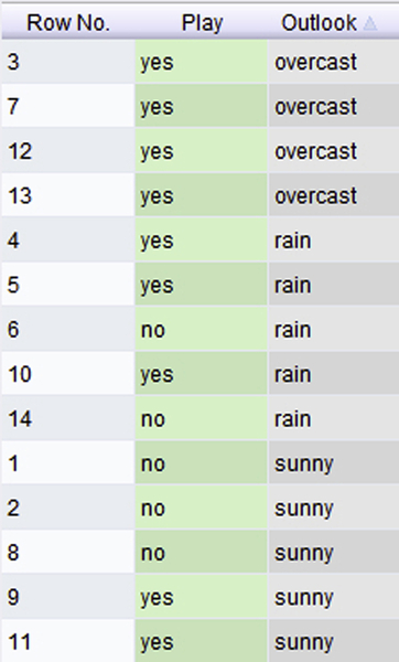
Before jumping into a business use case of decision trees, let us “implement” the decision tree model that was shown in Figure 4.4 on a small test sample using RapidMiner. Figure 4.5 shows the test data set, which is very much like our training data set but with small differences in attribute values.
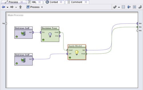
We have built a decision tree model using training data set. The RapidMiner process of building a decision tree is shown in Figure 4.6. More over, the same process shows the application of the decision tree model to test data set. When this process is executed, and the connections are made as shown inFigure 4.6, we get the table output shown in Figure 4.7. You can see that the model has been able to get 9 of the 14 class predictions correct and 5 of the 14 (in boxes) wrong, which translates to about 64% accuracy.
Figure 4.5Golf: Test data has a few minor differences in attribute values from the training data.
Let us examine a more involved business application to better understand how to apply decision trees for real world problems. Credit scoring is a fairly common predictive analytics problem. Some types of situations where credit scoring could be applied are:
1. Prospect filtering: Identify which prospects to extend credit to and determine how much credit would be an acceptable risk.
2. Default risk detection: Decide if a particular customer is likely to default on a loan.
3. Bad debt collection: Sort out those debtors who will yield a good cost (of collection) to benefit (of receiving payment) performance.
Figure 4.6Applying the simple decision tree model on unseen golf test data.
We will use the well-known German Credit data set from the University of California-Irvine Machine Learning data repository1 and describe how to use RapidMiner to build a decision tree for addressing a prospect filtering problem.
This is the first discussion of the implementation of a predictive analytics technique, so we will spend some extra effort in going into detail on many of the preliminary steps and also introduce several additional tools and concepts that will be required throughout the rest of this chapter and other chapters that focus on supervised learning methods. These are the concepts of splitting data into testing and training samples, and applying the trained model on testing (or validation data). It may also be useful to first review Sections 13.1 (Introduction to the GUI) and 13.2 (Data Import and Export) from Chapter 13 Getting Started with RapidMiner before working through the rest of this implementation. As a final note, we will not be discussing ways and means to improve the performance of a classification model using RapidMiner in this section, but will return to this very important part of predictive analytics in several later chapters, particularly in the section on using optimization in Chapter 13.
Figure 4.7Results of applying the simple decision tree model.
There are four main steps in setting up any supervised learning algorithm for a predictive modeling exercise:
1. Read in the cleaned and prepared data (see Chapter 2 Data Mining Process), typically from a spreadsheet, but the data can be from any source.
2. Split data into training and testing samples.
3. Train the decision tree using the training portion of the data set.
4. Apply the model on the testing portion of the data set to evaluate the performance of the model.
Step 1 may seem rather elementary, but can confuse many beginners and thus we will spend some time explaining this in somewhat more detail. The next few parts will describe other steps also in detail.
Step 1: Data Preparation
The raw data is in the format shown in Table 4.3. It consists of 1,000 samples and a total of 20 attributes and 1 label or target attribute. There are seven numeric attributes and the rest are categorical or qualitative, including the label, which is a binomial variable. The label attribute is called Credit Rating and can take the value of 1 (good) or 2 (bad). In the data 70% of the samples fall into the “good” credit rating class. The descriptions for the data are shown in Table 4.3. Most of the attributes are self-explanatory, but the raw data has encodings for the values of the qualitative variables. For example, attribute 4 is the purpose of the loan and can assume any of 10 values (A40 for new car, A41 for used car, and so on). The full details of these encodings are provided under the “Data Set Description” on the UCI-ML website.
Table 4.3
A View of the Raw German Credit data.
Checking Account Status
Duration in Month
Credit History
Purpose
Credit Amount
Savings Account/Bonds
Present Employment since
Credit Rating
A11
6
A34
A43
1169
A65
A75
1
A12
48
A32
A43
5951
A61
A73
2
A14
12
A34
A46
2096
A61
A74
1
A11
42
A32
A42
7882
A61
A74
1
A11
24
A33
A40
4870
A61
A73
2
A14
36
A32
A46
9055
A65
A73
1
A14
24
A32
A42
2835
A63
A75
1
A12
36
A32
A41
6948
A61
A73
1
A14
12
A32
A43
3059
A64
A74
1
A12
30
A34
A40
5234
A61
A71
2
A12
12
A32
A40
1295
A61
A72
2
A11
48
A32
A49
4308
A61
A72
2
RapidMiner’s easy interface allows quick importing of spreadsheets. A useful feature of the interface is the panel on the left, called the “Operators.” Simply typing in text in the box provided automatically pulls up all available RapidMiner operators that match the text. In this case, we need an operator to read an Excel spreadsheet, and so we simply type “excel” in the box. As you can see, the three Excel operators are immediately shown in Figure 4.8a: two for reading and one for exporting data.
Either double-click on the Read Excel operator or drag and drop it into the Main Process panel—the effect is the same, see Figure 4.8b. Once the Read Excel operator appears in the main process window, we need to configure the data import process. What this means is telling RapidMiner which columns to import, what is contained in the columns, and if any of the columns need special treatment.
This is probably the most “cumbersome” part about this step. RapidMiner has a feature to automatically detect the type of values in each attribute (Guess Value types). But it is a good exercise for the analyst to make sure that the right columns are picked (or excluded) and the value types are correctly guessed. If not, as seen in Figure 4.9, we can change the value type to the correct setting by clicking on the button below the attribute name.
Figure 4.8aUsing the Read Excel operator.
Figure 4.8bConfiguring the Read Excel operator.
Once the data is imported, we must assign the target variable for analysis, also known as a “label.” In this case, it is the Credit Rating, as shown in Figure 4.9. Finally it is a good idea to “run” RapidMiner and generate results to ensure that all columns are read correctly.
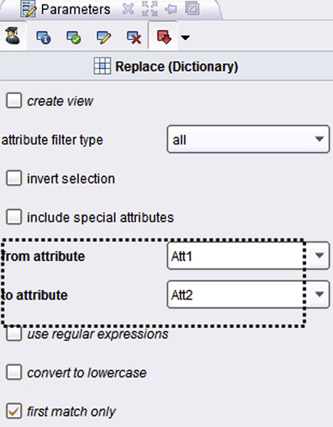
An optional step is to convert the values from A121, A143, etc. to more meaningful qualitative descriptions. This is accomplished by the use of another operator called Replace (Dictionary), which will replace the values with bland encodings such as A121 and so on with more descriptive values. We need to create a dictionary and supply this to RapidMiner as a comma-separated value (csv) file to enable this. Such a dictionary is easy to create and is shown inFigure 4.10a; the setup is shown in Figure 4.10b. Note that we need to let RapidMiner know which column in our dictionary contains old values and which contains new values.
Figure 4.9Verifying data read-in and adjusting attribute value types if necessary.
The last preprocessing step we show here is converting the numeric label (see Figure 4.9) into a binomial one by connecting the “exa”mple output of Replace (Dictionary) to a Numerical to Binominal operator. To configure the Numerical to Binominal operator, follow the setup shown in Figure 4.10c.
Finally, let us change the name of the label variable from Credit Rating to Credit Rating = Good so that it makes more sense when the integer values get converted to true or false after passing through the Numerical to Binomial operator. This can be done using the Rename operator. When we run this setup, we will generate the data set shown in Figure 4.11. Comparing to Figure 4.9, we will see that the label attribute is the first one shown and the values are “true” or “false.” We can examine the statistics tab of the results to get more information about the distributions of individual attributes and also to check for missing values and outliers. In other words, we must make sure that the data preparation step (Section 2.2) is properly executed before proceeding. In this implementation, we will not worry about this because the data set is relatively “clean” (for instance, there are no missing values), and we can proceed directly to the model development phase.
Figure 4.10aAttribute value replacement using a dictionary.
Figure 4.10bConfiguring the Replace (Dictionary) operator.
Figure 4.10cConvert the integer Credit Rating label variable to a binomial (true or false) type.
Step 2: Divide Data Set into Training and Testing Samples
As with all supervised model building, data must be separated into two sets: one for “training” or developing an acceptable model, and the other for “validating” or ensuring that the model would work equally well on a different data set. The standard practice is to split the available data into a training set and a testing or validation set. Typically the training set contains 70% to 90% of the original data. The remainder is set aside for testing or validation.
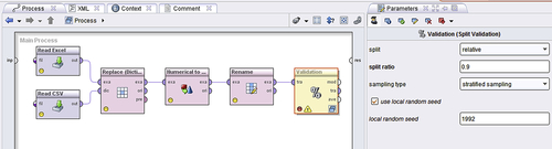
Figure 4.12 shows how to do this in RapidMiner. The Split Validation tool sets up splitting, modeling, and the validation check in one operator. The utility of this will become very obvious as you develop experience in data mining, but as a beginner, this may be a bit confusing.
Figure 4.11Data transformed for decision tree analysis.
Figure 4.12Using a relative split and a split ratio of 0.9 for training versus testing.
Choose stratified sampling with a split ratio of 0.9 (90% training). Stratified sampling will ensure that both training and testing samples have equal distributions of class values. (Although not necessary, it is sometimes useful to check the use local random seed option, so that it is possible to compare models between different iterations. Fixing the random seed ensures that the same examples are chosen for training (and testing) subsets each time the process is run.) The final sub step here is to connect the output from the Numerical to Binominal operator output to the Split Validation operator input.2
Step 3: Modeling Operator and Parameters
We will now see how to build a decision tree model on this data. As mentioned earlier, the Validation operator allows us to build a model and apply it on validation data in the same step. This means that two operations—model building and model evaluation—must be configured using the same operator. This is accomplished by double-clicking on the Validation operator, which is what is called a “nested” operator. All nested operators in RapidMiner have two little blue overlapping windows on the bottom right corner. When this operator is “opened,” we can see that there are two parts inside (see Figure 4.13). The left box is where the Decision Tree operator has to be placed and the model will be built using the 90% of training data samples. The right box is for applying this trained model on the remaining 10% of the testing data samples using the Apply Model operator and evaluating the performance of the model using the Performance operator.
Configuring the Decision Tree Model
The main parameters to pay attention to are the Criterion pull-down menu and the minimal gain box. This is essentially a partitioning criterion and offers information gain, Gini index, and gain ratio as choices. We covered the first two criteria earlier, and the gain ratio will be briefly explained in the next section.
Figure 4.13Setting up the split validation process.
As discussed earlier in this chapter, decision trees are built up in a simple five-step process by increasing the information contained in the reduced data set following each split. Data by its nature contains uncertainties. We may be able to systematically reduce uncertainties and thus increase information by activities like sorting or classifying. When we have sorted or classified to achieve the greatest reduction in uncertainty, we have basically achieved the greatest increase in information. We have seen how entropy is a good measure of uncertainty and how keeping track of it allows us to quantify information. So this brings us back to the options that are available within RapidMiner for splitting decision trees:
1. Information gain: Simply put, this is computed as the information before the split minus the information after the split. It works fine for most cases, unless you have a few variables that have a large number of values (or classes). Information gain is biased towards choosing attributes with a large number of values as root nodes. This is not a problem, except in extreme cases. For example, each customer ID is unique and thus the variable has too many values (each ID is a unique value). A tree that is split along these lines has no predictive value.
2. Gain ratio (default): This is a modification of information gain that reduces its bias and is usually the best option. Gain ratio overcomes the problem with information gain by taking into account the number of branches that would result before making the split. It corrects information gain by taking the intrinsic information of a split into account. Intrinsic information can be explained using our golf example. Suppose each of the 14 examples had a unique ID attribute associated with them. Then the intrinsic information for the ID attribute is given by 14 ∗ (–1/14 ∗ log (1/14)) = 3.807. The gain ratio is obtained by dividing the information gain for an attribute by its intrinsic information. Clearly attributes that have very high intrinsic information (high uncertainty) tend to offer low gains upon splitting and hence will not be automatically selected.
3. Gini index: This is also used sometimes, but does not have too many advantages over gain ratio.
4. Accuracy: This is also used to improve performance. The best way to select values for these parameters is by using many of the optimizing operators. This is a topic that will be covered in detail in Chapter 13.
The other important parameter is the minimal gain value. Theoretically this can take any range from 0 upwards. In practice, a minimal gain of 0.2 to 0.3 is considered good. The default is 0.1.
The other parameters (minimal size for a split, minimal leaf size, maximal depth) are determined by the size of the data set. In this case, we proceed with the default values. The best way to set these parameters is by using an optimization routine (which will be briefly introduced in Chapter 13 Getting Started with RapidMiner.
The last step in training the decision tree is to connect the input ports (“tra”ining) and output ports (“mod”el) as shown in the left (training) box of Figure 4.9. The model is ready for training. Next we add two more operators, Apply Model and Performance (Binominal Classification), and we are ready to run the analysis. Configure the Performance (Binominal Classification) operator by selecting the accuracy, AUC, precision, and recall options.3
Remember to connect the ports correctly as this can be a source of confusion:
▪ “mod”el port of the Testing window to “mod” on Apply Model
▪ “tes”ting port of the Testing window to “unl”abeled on Apply Model
▪ “lab”eled port of Apply Model to “lab”eled on Performance
▪ “per”formance port on the Performance operator to “ave”rageable port on the output side of the testing box
The final step before running the model is to go back to the main perspective by clicking on the blue up arrow on the top left (see Figure 4.13) and connect the output ports “mod”el and “ave” of the Validation operator to the main outputs.
Step 4: Process Execution and Interpretation
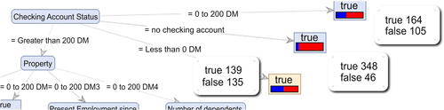
When the model is run as setup above, RapidMiner generates two tabs in the Results perspective (refer to Chapter 13 for the terminology). The PerformanceVector (Performance) tab shows a confusion matrix that lists the model accuracy on the testing data, along with the other options selected above for the Performance (Binominal Classification) operator in step 3. The Tree (Decision Tree) tab shows a graphic of the tree that was built on the training data (see Figure 4.14). Several important points must be highlighted before we discuss the performance of this model:
1. The root node—Checking Account Status—manages to classify nearly 94% of the data set. This can be verified by hovering the mouse over each of the three terminal leaves for this node. The total occurrences (of Credit Rating = Good: true and false) for this node alone are 937 out of 1000. In particular, if someone has a Checking Account Status = no checking account, then the chances of them having a “true” score is 88% (= 348/394, see Figure 4.15).
2. However, the tree is unable to clearly pick out true or false cases for Credit Rating = Good if Checking Account Status is Less than 0 DM (or Deutsche mark) (only a 51% chance of correct identification). A similar conclusion results if someone has 0 to 200 DM.
Figure 4.14A decision tree model for the prospect scoring data.
Figure 4.15Predictive power of the root node of the decision tree model.
3. If the Checking Account Status is greater than 200 DM, then the other parameters come into effect and play an increasingly important role in deciding if someone is likely to have a “good” or “bad” credit rating.
4. However, the fact that there are numerous terminal leaves with frequencies of occurrence as low as 2 (for example, “Present Employment since”), it implies that the tree suffers from overfitting. As described earlier, overfitting refers to the process of building a model very specific to the training data that achieves close to full accuracy on the training data. However when this model is applied on new data or if the training data changes somewhat, then there is a significant degradation in its performance. Overfitting is a potential issue with all supervised models, not just decision trees. One way we could have avoided this situation is by changing the decision tree criterion “Minimal leaf size” to something like 10 (instead of the default, 2). But doing so, we would also lose the classification influence of all the other parameters, except the root node [try it!]
Now let us look at the Performance result. As seen in Figure 4.16, the model’s overall accuracy on the testing data is 72%. The model has a class recall of 100% for the “true” class implying that it is able to pick out customers with good credit rating with 100% accuracy. However, its class recall for the “false” class is an abysmal 6.67%! That is, the model can only pick out a potential defaulter in 1 out of 15 cases!
One way to improve this performance is by penalizing false negatives by applying a cost for every such instance. This is handled by another operator called MetaCost, which is described in detail in Chapter 5 in the section on logistic regression. When we perform a parameter search optimization by iterating through three of the decision tree parameters, splitting criterion, minimum gain ratio, and maximal tree depth, we hit upon significantly improved performance as seen in Figure 4.17 below. More details on how to set this type of optimization are provided in Chapter 13.
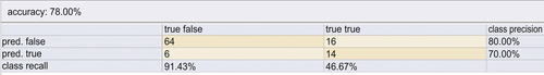
When we run the best model (described by the parameters on the top row of the table in Figure 4.17), we obtain the confusion matrix shown in Figure 4.18. Comparing this to Figure 4.16 we see that the recall for the more critical class (correctly identifying cases with a bad credit rating), has increased from about 7% to 91% whereas the recall for identifying a good credit rating has fallen below 50%. This may be acceptable in this particular situation if the costs of issuing a loan to a potential defaulter are significantly higher than the costs of losing revenue by denying credit to a creditworthy customer. The overall accuracy of the model is also higher than before.
Figure 4.16Baseline model performance measures.
Figure 4.17Optimizing the decision tree parameters to improve accuracy and class recall.
Figure 4.18Optimizing class recall for the credit default identification process.
In addition to assessing the model’s performance by aggregate measures such as accuracy, we can also use gain/lift charts, receiver operator characteristic (ROC) charts, and area under ROC curve (AUC) charts. An explanation of how these charts are constructed and interpreted is given in Chapter 8 on model evaluation.
The RapidMiner process for a decision tree covered in the implementation section can be accessed from the companion site of the book at www.LearnPredictiveAnalytics.com. The RapidMiner process (∗.rmp files) can be downloaded to the computer and imported to RapidMiner through File > Import Process. Additionally, all the data sets used in this book can be downloaded from www.LearnPredictiveAnalytics.com
4.1.3. Conclusions
Decision trees are one of the most commonly used predictive modeling algorithms in practice. The reasons for this are many. Some of the distinct advantages of using decision trees in many classification and prediction applications are explained below along with some common pitfalls.
▪ Easy to interpret and explain to nontechnical users
As we have seen in the few examples discussed so far, decision trees are very intuitive and easy to explain to nontechnical people, who are typically the consumers of analytics.
▪ Decision trees require relatively little effort from users for data preparation
There are several points that add to the overall advantages of using decision trees. If we have a data set consisting of widely ranging attributes, for example, revenues recorded in millions and loan age recorded in years, many algorithms require scale normalization before model building and application. Such variable transformations are not required with decision trees because the tree structure will remain the same with or without the transformation.
Another feature that saves data preparation time: missing values in training data will not impede partitioning the data for building trees. Decision trees are also not sensitive to outliers since the partitioning happens based on the proportion of samples within the split ranges and not on absolute values.
▪ Nonlinear relationships between parameters do not affect tree performance
As we describe in Chapter 5 on linear regression, highly nonlinear relationships between variables will result in failing checks for simple regression models and thus make such models invalid. However, decision trees do not require any assumptions of linearity in the data. Thus, we can use them in scenarios where we know the parameters are nonlinearly related.
▪ Decision trees implicitly perform variable screening or feature selection
We will discuss in Chapter 12 why feature selection is important in predictive modeling and data mining. We will introduce a few common techniques for performing feature selection or variable screening in that chapter. But when we fit a decision tree to a training data set, the top few nodes on which the tree is split are essentially the most important variables within the data set and feature selection is completed automatically. In fact, RapidMiner has an operator for performing variable screening or feature selection using the information gain ratio.
However, all these advantages need to be tempered with one key disadvantage of decision trees: without proper pruning or limiting tree growth, they tend to overfit the training data, making them somewhat poor predictors.