
4.5. Artificial Neural Networks
The objective of a predictive analytics algorithm is to model the relationship between input and output variables. The neural network technique approaches this problem by developing a mathematical explanation that closely resembles the biological process of a neuron. Although the developers of this technique have used many biological terms to explain the inner workings of neural network modeling process, it has a simple mathematical foundation. Consider the simple linear mathematical model:
![]()
Where Y is the calculated output and  are input attributes. 1 is the intercept and 2, 3, and 4 are the scaling factors or coefficients for the input attributes , respectively. We can represent this simple linear model in a topological form as shown in Figure 4.38.
In this topology, X1 is the input value and passes through a node, denoted by a circle. Then the value of X1 is multiplied by its weight, which is 2, as noted in the connector. Similarly, all other attributes (X2 and X3) go through a node and scaling transformation. The last node is a special case with no input variable; it just has the intercept. Finally, values from all the connectors are summarized in an output node that yields predicted output Y. The topology shown in Figure 4.38 represents the simple linear model  . The topology also represents a very simple artificial neural network (ANN). The neural networks model more complex nonlinear relationships of data and learn though adaptive adjustments of weights between the nodes. The ANN is a computational and mathematical model inspired by the biological nervous system. Hence, some of the terms used in an ANN are borrowed from biological counterparts.
In neural network terminology, nodes are called units. The first layer of nodes closest to the input is called the input layer or input nodes. The last layer of nodes is called the output layer or output nodes. The output layer performs an aggregation function and also can have a transfer function. The transfer function scales the output into the desired range. Together with the aggregation and transfer function, the output layer performs an activation function. This simple two-layer topology, as shown in Figure 4.38, with one input and one output layer is called a perceptron, the most simplistic form of artificial neural network. A perceptron is a feed-forward neural network where the input moves in one direction and there are no loops in the topology.

Biological Neurons
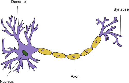
The functional unit of cells in the nervous system is the neuron. An artificial neural network of nodes and connectors has a close resemblance to a biological network of neurons and connections, with each node acting as a single neuron. There are close to 100 billion neurons in the human brain and they are all interconnected to form this very important organ of the human body (see Figure 4.39). Neuron cells are found in most animals; they transmit information through electrical and chemical signals. The interconnection between one neuron with another neuron happens through a synapse. A neuron consists of a cell body, a thin structure that forms from the cell body called dendrite, and a long linear cellular extension called an axon. Neurons are composed of a number of dendrites and one axon. The axon of one neuron is connected to the dendrite of another neuron through a synapse, and electrochemical signals are sent from one neuron to another. There are about 100 trillion synapses in a human brain.

A artificial neural network is typically used for modeling nonlinear, complicated relationships between input and output variables. This is made possible by the existence of more than one layer in the topology, apart from the input and output layers, called hidden layers. A hidden layer contains a layer of nodes that connects input from previous layers and applies an activation function. The output is now calculated by a more complex combination of input values, as shown in Figure 4.40.
Consider the example of the Iris data set. It has four input variables, sepal length, sepal width, petal length, and petal width, with three classes (Iris setosa, Iris versicolor, Iris virginica) in the label. An ANN based on the Iris data set yields a three-layer structure (the number of layers can be specified by the user) with three output nodes, one for each class variable. For a categorical label problem, as in predicting species for Iris, the ANN provides output for each class type. A winner class type is picked based on the maximum value of the output class label. The topology in Figure 4.40 is a feed-forward artificial neural network with one hidden layer. Of course, depending on the problem to be solved, we can use a topology with multiple hidden layers and even with looping where the output of one layer is used as input for preceding layers. Specifying what topology to use is a challenge in neural network modeling and it takes time to build a good approximating model.
The activation function used in the output node consists of a combination of an aggregation function, usually summarization, and a transfer function. Transfer functions can be anything from sigmoid to normal bell curve, logistic, hyperbolic, or linear functions. The purpose of sigmoid and bell curves is to provide a linear transformation for a particular range of values and a nonlinear transformation for the rest of the values. Because of the transformation function and the presence of multiple hidden layers, we can model or closely approximate almost any mathematical continuous relationship between input variables and output variables. Hence, a multilayer artificial neural network is called a universal approximator. However, the presence of multiple user options such as topology, transfer function, and number of hidden layers makes the search for an optimal solution quite time consuming.
4.5.1. How It Works
An artificial neural network learns the relationship between input attributes and the output class label through a technique called back propagation. For a given network topology and activation function, the key training task is to find the weights of the links. The process is rather intuitive and closely resembles the signal transmission in biological neurons. The model uses every training record to estimate the error of the predicted output as compared against the actual output. Then the model uses the error to adjust the weights to minimize the error for the next training record and this step is repeated until the error falls within the acceptable range (Laine, 2003). The rate of correction from one step to other should be managed properly, so that the model does not overcorrect. Following are the key steps in developing an artificial neural network from a training data set.


Step 1: Determine the Topology and Activation Function
For this example, let’s assume a data set with three numeric input attributes (X1, X2, X3) and one numeric output (Y). To model the relationship, we are using a topology with two layers and a simple aggregation activation function, as shown in Figure 4.41. There is no transfer function used in this example.
Step 2: Initiation
Let’s assume the initial weights for the four links are 1, 2, 3, and 4. Let’s take an example model and a test record with all the inputs as 1 and the known output as 15. So, X1 = X2 = X3 = 1 and output Y = 15. Figure 4.42 shows initiation of first training record.
Step 3: Calculating Error
We can calculate the predicted output of the record from Figure 4.42. This is simple feed forward process of passing through the input attributes and calculating the predicted output. The predicted output  according to current model is 1 + 1 ∗ 2 + 1 ∗ 3 + 1 ∗ 4 = 10. The difference between the actual output from training record and predicted output is the error:

![]()
The error for this example training record is 15 – 10 = 5.
Step 4: Weight Adjustment
Weight adjustment is the most important part of learning in an artificial neural network. The error calculated in the previous step is passed back from the output node to all other nodes in the reverse direction. The weights of the links are adjusted from their old value by a fraction of the error. The fraction λ applied to the error is called learning rate. λ takes values from 0 to 1. A value close to 1 results in a drastic change to the model for each training record and a value close to 0 results in smaller changes and less correction. New weight of the link (w) is the sum of old weight (w’) and the product of learning rate and proportion of the error (λ ∗ e).
![]()
The choice of λ can be tricky in the implementation of an ANN. Some model processes start with λ close to 1 and reduce the value of λ while training each cycle. By this approach any outlier records later in the training cycle will not degrade the relevance of the model. Figure 4.43 shows the error propagation in the topology.
The current weight of the first link is w2 = 2. Let’s assume the learning rate is 0.5. The new weight will be w2 = 2 + 0.5 ∗ 5/3 = 2.83. The error is divided by 3 because the error is back propagated to three links from the output node. Similarly, the weight will be adjusted for all the links. In the next cycle, a new error will be computed for the next training record. This cycle goes on until all the training records are processed by iterative runs. The same training example can be repeated until the error rate is less than a threshold. We have reviewed a very simple case of an artificial neural network. In reality, there will be multiple hidden layers and multiple output links—one for each nominal class value. Because of the numeric calculation, an ANN model works well with numeric inputs and outputs. If the input contains a nominal attribute, a preprocessing step should be included to convert the nominal attribute into multiple numeric attributes—one for each attribute value, this process is similar to dummy variable introduction, which will be further explored in chapter 10 Time Series Forecasting. This specific preprocessing increases the number of input links for neural network in the case of nominal attributes and thus increases the necessary computing resources. Hence, an ANN is more suitable for attributes with a numeric data type.
4.5.2. How to Implement
An artificial neural network is one of the most popular algorithms available for data mining tools. In RapidMiner, the ANN model operators are available in the Classification folder. There are three types of models available: A simple perceptron with one input and one output layer, a flexible ANN model called Neural Net with all the parameters for complete model building, and advanced AutoMLP algorithm. AutoMLP (for Automatic Multilayer Perceptron) combines concepts from genetic and stochastic algorithms. It leverages an ensemble group of ANNs with different parameters like hidden layers and learning rates. It also optimizes by replacing the worst performing models with better ones and maintains an optimal solution. For the rest of the discussion, we will focus on the Neural Net model.
Step 1: Data Preparation
The Iris data set is used to demonstrate the implementation of an ANN. All four attributes for the Iris data set are numeric and the output has three classes. Hence the ANN model will have four input nodes and three output nodes. The ANN model will not work with categorical or nominal data types. If the input has nominal attributes, it should be converted to numeric using data transformation, see Chapter 13 Getting Started with RapidMiner. Nominal to binominal conversion operator can be used to convert each value of a nominal attribute to separate binominal attributes. In this example, we use the Rename operator to name the four attributes of the Iris data set and the Split Data operator to split 150 Iris records equally into the training and test data.
Step 2: Modeling Operator and Parameters
The training data set is connected to the Neural Net operator (Modeling > Classification and Regression > Neural Net Training). The Neural Net operator accepts real values and later converts them into the normalized range –1 to 1 and outputs a standard ANN model. The following parameters are available in ANN for users to change and customize in the model.
▪ Hidden layer: Determines the number of layers, size of each hidden layer, and names of each layer for easy identification in the output screen. The default size of the node is –1, which is actually calculated by (number of attributes + number of classes)/2 + 1. The default can be overwritten by specifying an integer of nodes, not including a no-input threshold node per layer.
▪ Training cycles: This number of times a training cycle is repeated; it defaults to 500. In a neural network, every time a training record is considered, the previous weights are quite different and hence it is necessary to repeat the cycle many times.
▪ Learning rate: The value of λ determines how sensitive the change in weight has to be in considering error for the previous cycle. It takes a value from 0 to 1. A value closer to 0 means the new weight would be more based on the previous weight and less on error correction. A value closer to 1 would be mainly based on error correction.
▪ Decay: During the neural network training, ideally the error would be minimal in the later portion of the record sequence. We don’t want a large error due to any outlier records in the last few records, thereby impacting the performance of the model. Decay reduces the value of the learning rate and brings it closer to zero for the last training record.
▪ Shuffle: If the training record is sorted, we can randomize the sequence by shuffling it. The sequence has an impact in the model, particularly if the group of records exhibiting nonlinear characteristics are all clustered together in the last segment of the training set.
▪ Normalize: Nodes using a sigmoid transfer function expect input in the range of –1 to 1. Any real value of the input should be normalized in an ANN model.
▪ Error epsilon: The objective of the ANN model should be to minimize the error but not make it zero, at which the model memorizes the training set and degrades the performance. We can stop the model building process when the error is less than a threshold called the error epsilon.
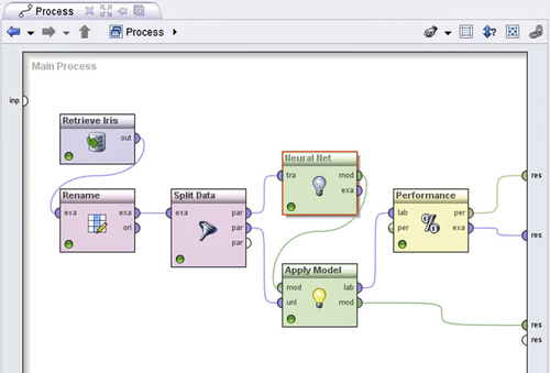
The output of the Neural Net operator can be connected to the Apply Model operator, which is standard in every predictive analytics workflow. The Apply Model operator also gets an input data set from the Split data operator for the test data set. The output of the Apply Model operator is the labeled test data set and the ANN model.
Step 3: Evaluation
The labeled data set output after using the Apply Model operator is then connected to the Performance – Classification operator (Evaluation > Performance Measurement > Performance), to evaluate the performance of the classification model. Figure 4.44 shows the complete artificial neural network predictive classification process. The output connections can be connected to the result ports and the process can be saved and executed.
Step 4: Execution and Interpretation
The output results window for the model provides a visual on the topology of the ANN model. Figure 4.45 shows the model output topology. Upon a click on a node, we can get the weights of the incoming links to the node. The color of the link indicates relative weights. The description tab of the model window provides the actual values of the link weights.
The output performance vector can be examined to see the accuracy of the artificial neural network model built for the Iris data set. Figure 4.46 shows the performance vector for the model. A three-layer ANN model with the default parameter options and equal splitting of input data and training set yields 93% accuracy. Out of 75 examples, only 5 were misclassified.


4.5.3. Conclusion
Neural network models require strict preprocessing. If the test example has missing attribute values, the model cannot function, similar to regression or decision trees. The missing values can be replaced with average values or any default values to minimize the error. The relationship between input and output cannot be explained clearly by an artificial neutral network. Since there are hidden layers, it is quite complex to understand the model. In many data mining applications explanation of the model is as important as prediction itself. Decision trees, induction rules, and regression do a far better job at explaining the model.
Building a good ANN model with optimized parameters takes time. It depends on the number of training records and iterations. There are no consistent guidelines on the number of hidden layers and nodes within each hidden layer. Hence, we would need to try out many parameters to optimize the selection of parameters. However, once a model is built, it is straightforward to implement and an example record gets classified quite fast.
An ANN does not handle categorical input data. If the data has nominal values, it needs to be converted to binary or real values. This means one input attribute explodes to multiple input attributes and exponentially increases nodes, links, and complexity. Also, converting nonordinal categorical data, like zip code, to numeric provides an opportunity for ANN to make numeric calculations, which doesn’t quite make sense. Having redundant correlated attributes is not going to be a problem in an ANN model. If the example set is large, having outliers will not degrade the performance of the model. However, outliers will impact the normalization of the signal, which most ANN models require for input attributes. Because model building is by incremental error correction, ANN can yield local optima as the final model. This risk can be mitigated by managing a momentum parameter to weigh the update.
Although model explanation is quite difficult with an ANN, the rapid classification of test examples makes an ANN quite useful for anomaly detection and classification problems. An ANN is commonly used in fraud detection, a scoring situation where the relationship between inputs and output is nonlinear. If there is a need for something that handles a highly nonlinear landscape along with fast real-time performance, then the artificial neural network is a good option.
..................Content has been hidden....................
You can't read the all page of ebook, please click here login for view all page.